Abstract

Schubert calculus provides algebraic tools to solve enumerative problems. There have been several applied problems in systems theory, linear algebra and physics which were studied by means of Schubert calculus. The method is most powerful when the base field is algebraically closed. In this article we first review some of the successes Schubert calculus had in the past. Then we show how the problem of decoding of subspace codes used in random network coding can be formulated as a problem in Schubert calculus. Since for this application the base field has to be assumed to be a finite field new techniques will have to be developed in the future.

1 Introduction

Hermann Cäsar Hannibal Schubert (1848-1911) is considered the founder of enumerative geometry. He was a high school teacher in Hamburg, Germany. He studied questions of the type: Given four lines in projective three-space in general position, is there a line intersecting all given ones. This question can then be generalized to:

Problem 1.

Given $N$ $k$-dimensional subspaces $\mathcal{U}_{i}\subset\mathbb{C}^{k+m}$. Is there a subspace $\mathcal{V}\subset\mathbb{C}^{k+m}$ of complimentary dimension $m=\dim V$ such that

$$\mathcal{V}\bigcap\mathcal{U}_{i}\neq\{0\},\ i=1,\ldots,N.$$ (1)

Using a symbolic calculus he then came up with the following surprising result [21, 22]:

Theorem 2.

In case the subspaces $\mathcal{U}_{i}\subset\mathbb{C}^{k+m},i=1,\ldots,N$ are in general position and in case $N=km$ there exist exactly

$$d(k,m)=\frac{1!2!\cdots(k-1)!(km)!}{m!(m+1)!\cdots(m+k-1)!}.$$ (2)

different $m$ dimensional subspaces $\mathcal{V}\subset\mathbb{C}^{k+m}$ which satisfy the intersection condition $($1$)$.

Note that two-dimensional subspaces in $\mathbb{C}^{4}$ describe lines in projective space $\mathbb{P}^{3}$ and Schubert hence claims in the case of four lines in three-space in general position that there are exactly $d(2,2)=2$ lines intersecting all four given lines.

Schubert used in the derivation of Theorem 2 Poncelet’s principle of preservation of numbers which was not considered a theorem of mathematics at the time. For this reason Schubert’s results were not accepted by the mathematics community of the 19th century and Hilbert devoted the 15th of his famous 24 problems to the question if mathematicians can come up with rigorous techniques to prove or disprove the claims of Dr. Schubert. A rigorous verification of Theorem 2 was derived in the last century and we refer the interested reader to the survey article [14] by Kleiman, where the progress over time about Schubert calculus and the Hilbert problem 15 is described.

In the sequel we introduce the most important concepts from Schubert calculus.

Let $\mathbb{F}$ be an arbitrary field. Denote by ${\rm Grass}(k,n)={\rm Grass}(k,\mathbb{F}^{n})$ the Grassmann variety consisting of all $k$-dimensional subspaces of the vector space $\mathbb{F}^{n}$. ${\rm Grass}(k,n)$ can be embedded into projective space using the Plücker embedding:

$$\varphi:{\rm Grass}(k,\mathbb{F}^{n}) \longrightarrow\mathbb{P}^{\binom{n}{k}-1}$$

$$\mathrm{span}(u_{1},\ldots,u_{k}) \longmapsto\mathbb{F}(u_{1}\wedge\ldots\wedge u_{k}).$$

If one chooses a basis $\{e_{1},\ldots,e_{n}\}$ of $\mathbb{F}^{n}$ and the corresponding canonical basis of $\Lambda^{k}\mathbb{F}^{n}$

$$\{e_{i_{1}}\wedge\ldots\wedge e_{i_{k}}\mid 1\leq i_{1}<\ldots<i_{k}\leq n\}$$

then one has an induced map of the coordinates. If $U$ is a $k\times n$ matrix whose row space $\mathrm{rs}(U)$ describes the subspace $\mathcal{U}:=\mathrm{span}(u_{1},\ldots,u_{k})$ and $U[i_{1},\dots,i_{k}]$ denotes the submatrix of $U$ given by the columns $i_{1},\dots,i_{k}$, then one readily verifies that the Plücker embedding is given in terms of coordinates via:

$$\mathrm{rs}(U)\longmapsto[\det(U[1,...,k]):\det(U[1,...,k-1,k+1]):...:\det(U[n-k+1,...,n]).$$

The $k\times k$ minors $\det(U[i_{1},\ldots,i_{k}])$ of the matrix $U$ are called the Plücker coordinates of the subspace $\mathcal{U}$.

The image of this embedding describes indeed a variety and the defining equations are given by the so called “shuffle relations” (see e.g. [15, 19]). The shuffle relations are a set of quadratic equations in terms of the Plücker coordinates.

A flag ${\mathcal{F}}$ is a sequence of nested linear subspaces

$${\mathcal{F}}:\ \{0\}\subset V_{1}\subset V_{2}\subset\ldots\subset V_{n}={\mathbb{F}}^{n}$$

having the property that $\dim V_{j}=j$ for $j=1,\dots,n$.

Denote by $\nu=(\nu_{1},\ldots,\nu_{k})$ an ordered index set satisfying

$$1\leq\nu_{1}<\ldots<\nu_{k}\leq n.$$

For every flag ${\mathcal{F}}$ one defines a Schubert variety

$$\hskip 17.07164ptS(\nu;\mathcal{F}):=\{W\in{\rm Grass}(m,\mathbb{F}^{n})\mid\dim(W\bigcap V_{\nu_{i}})\geq i\ \mbox{ for }i=1,\ldots,k\}.$$ (3)

The Schubert varieties are sub-varieties of the Grassmannian ${\rm Grass}(k,\mathbb{F}^{n})$ and they contain a Zariski dense affine subset called Schubert cell and defined as:

$$C(\nu;\mathcal{F}):=\{W\in S(\nu;\mathcal{F})\mid\dim(W\bigcap V_{\nu_{i}-1})=i-1;\mbox{ for }i=1,\ldots,k\}.$$ (4)

In terms of Plücker coordinates the defining equations of the Schubert variety $S(\nu;\mathcal{F})$ are given by the quadratic shuffle relations describing the Grassmann variety together with a set of linear equations (see [15]).

A fundamental question in Schubert calculus is now the following:

Problem 3.

Given two Schubert varieties $S(\nu;\mathcal{F})$ and $S(\tilde{\nu};\tilde{\mathcal{F}})$. Describe as explicitly as possible the intersection variety

$$S(\nu;\mathcal{F})\cap S(\tilde{\nu};\tilde{\mathcal{F})}.$$

Schubert’s Theorem 2 can actually also be formulated as an intersection problem of Schubert varieties. For this note that

$$\left\{\mathcal{V}\in{\rm Grass}(k,\mathbb{F}^{k+m})\mid\mathcal{V}\bigcap\mathcal{U}_{i}\neq\{0\}\right\}$$ (5)

describes a Schubert variety with regard to some flag and the theorem then states that in the intersection of $N$ Schubert varieties of above type one finds $d(k,m)$ $m$-dimensional subspaces as solutions in general.

In the case of an algebraically closed field one has rather precise information about this intersection variety. Topologically the intersection variety turns out to be a union of Schubert varieties of lower dimension and the multiplicities are governed by the Littlewood–Richardson rule [9]. When the field is not algebraically closed much less is known. There has been work done over the real numbers by Frank Sottile [25, 26]. Over general fields very little is known and we will show in this article that the decoding of subspace codes can be viewed as a Schubert calculus problem over some finite field. The following example illustrates the concepts.

Example 4.

As a base field we take $\mathbb{F}=\mathbb{F}_{2}=\{0,1\}$ the binary field. Consider the Grassmannian ${\rm Grass}_{2}(2,\mathbb{F}^{4})$ representing all lines in projective three-space $\mathbb{P}^{3}$. We would like to study Schubert’s question in this situation: Given four lines in three-space, is there always a line intersecting all four given ones. Clearly there are many situations where the answer is affirmative, e.g. when the lines already intersect in some point. In general this is however not the case as we now demonstrate. Consider the following four lines in $\mathbb{P}^{3}$ represented as row spaces of the following four matrices:

$$\left[\begin{array}[]{cccc}1&0&0&0\\ 0&1&0&0\end{array}\right],\left[\begin{array}[]{cccc}0&0&1&0\\ 0&0&0&1\end{array}\right],\left[\begin{array}[]{cccc}1&1&0&1\\ 0&1&1&1\end{array}\right],\left[\begin{array}[]{cccc}1&1&1&0\\ 1&0&1&1\end{array}\right].$$

We claim that there exists no line in projective three-space $\mathbb{P}^{3}$, i.e. no two-dimensional subspace in ${\rm Grass}_{2}(2,\mathbb{F}^{4})$ intersecting all four given subspaces non-trivially.

${\rm Grass}_{2}(2,\mathbb{F}^{4})$ is embedded in $\mathbb{P}^{5}$ via the Plücker embedding. Denote by

$$u_{i,j}:=\det U[i,j],1\leq i<j\leq 4$$

the Plücker coordinates of some subspace $\mathcal{U}\in{\rm Grass}_{2}(2,\mathbb{F}^{4})$. The four lines impose the linear constraints:

$$u_{3,4} = 0,$$

$$u_{1,2} = 0,$$

$$u_{1,2}+u_{1,4}+u_{2,3}+u_{2,4}+u_{3,4} = 0,$$

$$u_{1,2}+u_{1,3}+u_{1,4}+u_{2,3}+u_{3,4} = 0.$$

The points in $\mathbb{P}^{5}$ representing the image of ${\rm Grass}_{2}(2,\mathbb{F}^{4})$ are described by one quadratic equation (shuffle relation):

$$u_{1,2}u_{3,4}+u_{1,3}u_{2,4}+u_{1,4}u_{2,3}=0.$$

Solving the 5 equations in the 6 unknowns results in one quadratic equation:

$$(u_{1,4})^{2}+u_{1,4}u_{2,3}+(u_{2,3})^{2}=0$$

which has no solutions over $\mathbb{F}_{2}$ in $\mathbb{P}^{5}$. Note that there are exactly $d(2,2)=2$ solutions over the algebraic closure as predicted by Schubert.

Readers who want to know more on the subject of Schubert calculus will find material in the survey article [15].

The paper is structured as follows: In Section 2 we present results which were derived by Schubert calculus. In Section 3 we introduce the main topic of this paper, namely subspace codes used in random network coding. In Section 4 we show that list decoding of random network codes is a problem of Schubert calculus over some finite field.

2 Results in Systems Theory and Linear Algebra Derived by Means of Schubert Calculus

In the past Schubert calculus has been a very powerful tool for several problem areas in the applied sciences. In this section we review two such problem areas and we show to what extend Schubert calculus led to strong existence results and better understanding.

The pole placement problem

One of the most prominent problems in mathematical systems theory has been the pole placement problem. In the static situation the problem can be described as follows: Consider a discrete linear system

$$x(t+1)=Ax(t)+Bu(t),\ \ y(t)=Cx(t)$$ (6)

described by matrices $A,B,C$ having size $n\times n$, $n\times m$ and $p\times n$ respectively. Consider a monic polynomial

$$\varphi(s):=s^{n}+a_{n-1}s^{n-1}+\cdots+a_{1}s+a_{0}\in\mathbb{F}[s]$$

of degree $n$ having coefficients in the base field $\mathbb{F}$. In its simplest version the pole placement problem asks for the existence of a feedback law $u(t)=Ky(t)$ such that the resulting closed loop system

$$x(t+1)=\left(A+BKC\right)x(t)$$ (7)

has characteristic polynomial $\varphi(s)$.

At first glance this problem looks like a problem from matrix theory whose solution can be derived by means of linear algebra. Surprisingly, the problem is highly nonlinear and closely related to Schubert’s Problem 1. This geometric connection was first realized in an interesting paper by Brockett and Byrnes [2] who showed that over the complex numbers arbitrary pole placement is generically possible as soon as $n\leq mp$ and in case that the McMillan degree $n$ is equal to $mp$ then there are exactly $d(m,p)$ static feedback laws resulting in the closed loop characteristic polynomial $\varphi(s)$. The interested reader will find more details in a survey article by Byrnes [3].

The geometric insight one gained from the Grassmannian point of view was also helpful for deriving pole placement results over other base field. Over the reals the most striking result was obtained by A. Wang in [31] where it was shown that arbitrary pole placement is possible with real compensators as soon as $n<mp$. Over a finite field some preliminary results were obtained by Gorla and the first author in [7].

U. Helmke in collaboration with X. Wang and the first author have been studying the pole placement problem in the situation when symmetries are involved [10]. This problem then leads to a Schubert type problem in the Lagrangian Grassmannian.

Sums of Hermitian matrices

Given Hermitian matrices $A_{1},\ldots,A_{r}\in\mathbb{C}^{n\times n}$ each with a fixed spectrum

$$\lambda_{1}(A_{l})\geq\ldots\geq\lambda_{n}(A_{l}),\ \ l=1,\ldots,r$$ (8)

and arbitrary else. Is it possible to find then linear inequalities which describe the possible spectrum of the Hermitian matrix

$$A_{r+1}:=A_{1}+\cdots+A_{r}?$$

Questions of this type have a long history in operator theory and linear algebra. For example H. Weyl derived in 1912 the following famous inequality for any set of indices $1\leq i,j\leq n$ with $1\leq i+j-1\leq n$:

$$\lambda_{i+j-1}(A_{1}+A_{2})\leq\lambda_{i}(A_{1})+\lambda_{j}(A_{2}).$$ (9)

In collaboration with U. Helmke the first author extended work by Johnson [13] and Thompson [28, 27] to derive a large set of eigenvalue inequalities. This was achieved through the use of Schubert calculus and we will say more in a moment. The obtained inequalities included in special cases not only the inequalities by H. Weyl but also the more extensive inequalities from Lidskii and Freede Thompson [28].

In order to make the connection to Schubert calculus we follow [9] and denote with $v_{1l},\ldots,v_{nl}$ the set of orthogonal eigenvectors of the Hermitian operator $A_{l}$, $l=1,\ldots,r+1$.

Using these ordered set of eigenvectors one constructs for each Hermitian matrix $A_{l}$ the flag:

$${\cal F}_{l}:\hskip 11.38109pt\{0\}\subset V_{1l}\subset V_{2l}\subset\ldots\subset V_{nl}=\mathbb{C}^{n}$$ (10)

defined through the property:

$$V_{ml}:={\rm span}(v_{1l},\ldots,v_{ml})\;\;m=1,\dots,n.$$ (11)

The connection to Schubert calculus is now established by the following result as it can be found in [9]. The theorem generalizes earlier results by Freede and Thompson [28].

Theorem 5.

Let $A_{1},\ldots,A_{r}$ be complex Hermitian $n\times n$ matrices and denote with ${\mathcal{F}}_{1},\ldots,{\mathcal{F}}_{r+1}$ the corresponding flags of eigenspaces defined by $($11$)$. Assume $A_{r+1}=A_{1}+\cdots+A_{r}$. and let $\underline{i}_{l}=(i_{1l},\ldots,i_{kl})$ be $r+1$ sequences of integers satisfying

$$1\leq i_{1l}<\ldots<i_{kl}\leq n,\hskip 5.69054ptl=1,\ldots,r+1.$$ (12)

Suppose the intersection of the $r+1$ Schubert subvarieties of ${\rm Grass}(k,\mathbb{C}^{n})$ is nonempty, i.e.:

$$S(\underline{i}_{1};{\cal F}_{1})\bigcap\ldots\bigcap S(\underline{i}_{r+1};{\cal F}_{r+1})\neq\emptyset.$$ (13)

Then the following matrix eigenvalue inequalities hold:

$$\sum_{j=1}^{k}\lambda_{n-i_{j,r+1}+1}(A_{1}+\cdots+A_{r})\geq\sum_{l=1}^{r}\sum_{j=1}^{k}\lambda_{i_{jl}}(A_{l})$$ (14)

$$\sum_{j=1}^{k}\lambda_{i_{j,r+1}}(A_{1}+\cdots+A_{r})\leq\sum_{l=1}^{r}\sum_{j=1}^{k}\lambda_{n-i_{jl}+1}(A_{l}).$$ (15)

In 1998 Klyachko could show that the inequalities coming from Schubert calculus as described in Theorem 5 are not only necessary but that they describe a Polytope of all possible inequalities. The interested reader will find Klyachko’s result as well as much more in the survey article by Fulton [6].

A priori classical Schubert calculus provides very strong existence results. It is a different matter to derive effective numerical algorithms to compute the subspaces which satisfy the different Schubert conditions. For this reason Huber, Sottile and Sturmfels [12] developed effective numerical algorithms over the reals. As we will demonstrate in the next sections it would be very desirable to have effective numerical algorithms also in the case of Schubert type problems defined over some finite field.

3 Random Network Coding

In network coding one is looking at the transmission of information through a network with possibly several senders and several receivers. A lot of real-life applications of network coding can be found, e.g. data streaming over the Internet, where a source wants to send the same information to many receivers at the same time.

The network channel is represented by a directed graph with three different types of vertices, namely sources, i.e. vertices with no incoming edges, sinks, i.e. vertices with no outgoing edges, and inner nodes, i.e. vertices with incoming and outgoing edges. One assumes that at least one source and one sink exist. Under linear network coding the inner nodes are allowed to forward linear combinations of the incoming information vectors. The use of linear network coding possibly improves the transmission rate in comparison to just forwarding information at the inner nodes [1]. This can be illustrated in the example of the butterfly network:

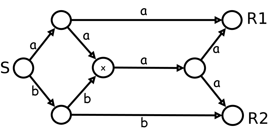
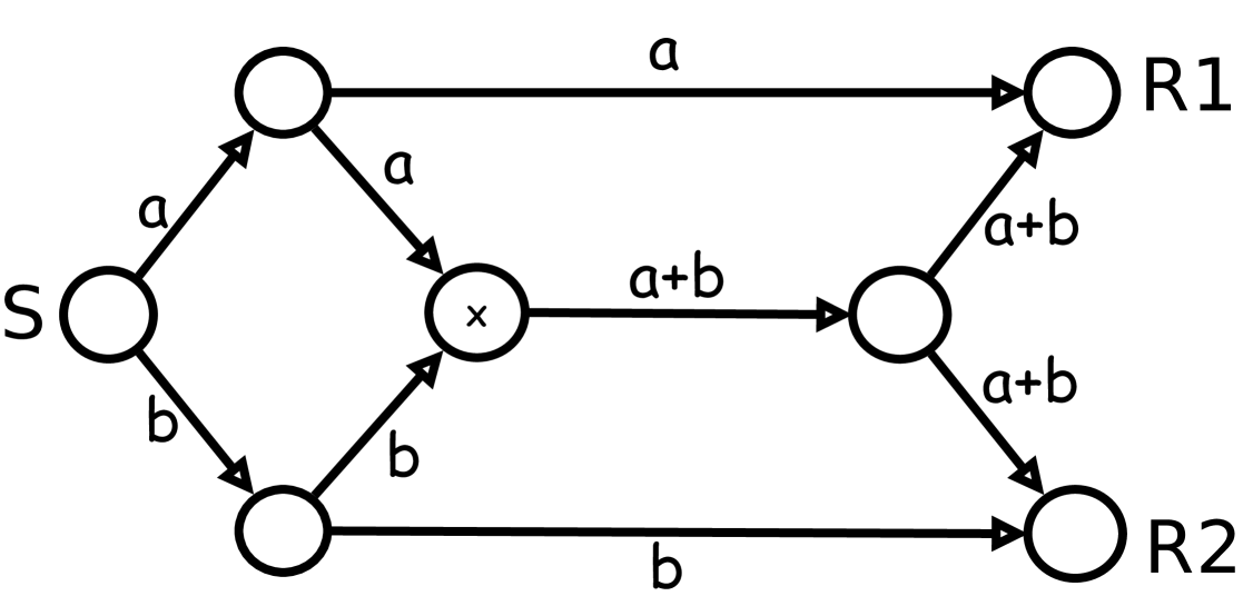
Figure 1: The butterfly network under the forwarding and the network coding model.

The source $S$ wants to send the same information, $a$ and $b$, to both receivers $R1$ and $R2$. Under forwarding every inner node forwards the incoming information and thus has to decide on either $a$ or $b$ (in this example on $a$) at the bottleneck vertex, marked above by x. Thus, $R1$ does not receive $b$. With linear network coding we allow the bottleneck vertex to send the sum of the two incoming informations, which allows both receivers to recover both $a$ and $b$ with a simple operation.

In this linear network coding setting, when the topology of the underlying network is unknown or time-varying, one speaks of random (linear) network coding. This setting was first studied in [11] and a mathematical model was introduced in [17], where the authors showed that it makes sense to use vector spaces instead of vectors over a finite field $\mathbb{F}_{q}$ as codewords. In this model the source injects a basis of the respective codeword into the network and the inner nodes forward a random linear combination of their incoming vectors. Therefore, each sink receives a linear combinations of the original vectors, which span the same vector space as the sent vectors, if no errors occurred during transmission.

In coding practice the base field is a finite field $\mathbb{F}_{q}$ having $q$ elements, where $q$ is a prime power. $\mathbb{F}_{q}^{\times}:=\mathbb{F}_{q}\setminus\{0\}$ will denote the set of all invertible elements of $\mathbb{F}_{q}$. We will call the set of all subspaces of $\mathbb{F}_{q}^{n}$ the projective geometry of $\mathbb{F}_{q}^{n}$, denoted by $\mathcal{P}(q,n)$, and denote the Grassmannian $\mathrm{Grass}(k,\mathbb{F}_{q}^{n})$ by $\mathrm{Grass}_{q}(k,n)$.

There are two types of errors that may occur during transmission, a decrease in dimension which is called an erasure and an increase in dimension, called an insertion. Assume $\mathcal{U}\in\mathcal{P}(q,n)$ was sent and erasures and insertions occurred during transmission, then the received word is of the type

$$\mathcal{R}=\bar{\mathcal{U}}\oplus\mathcal{E}$$

where $\bar{\mathcal{U}}$ is a subspace of $\mathcal{U}$ and $\mathcal{E}\in\mathcal{P}(q,n)$ is the error space. A random network coding channel in which both insertions and erasures can happen is called an operator channel.

In order to have a notion of decoding capability of some code a good metric is required on the set $\mathcal{P}(q,n)$: The subspace distance is a metric on $\mathcal{P}(q,n)$ given by

$$d_{S}(\mathcal{U},\mathcal{V})= \dim(\mathcal{U}+\mathcal{V})-\dim(\mathcal{U}\cap\mathcal{V})$$

$$= \dim(\mathcal{U})+\dim(\mathcal{V})-2\dim(\mathcal{U}\cap\mathcal{V})$$

for any $\mathcal{U},\mathcal{V}\in\mathcal{P}(q,n)$. Another metric on $\mathcal{P}(q,n)$ is the injection distance, defined as

$$d_{I}(\mathcal{U},\mathcal{V})= \max\{\dim(\mathcal{U}),\dim(\mathcal{V})\}-\dim(\mathcal{U}\cap\mathcal{V}).$$

Note, that for $\mathcal{U},\mathcal{V}\in\mathrm{Grass}_{q}(k,n)$ it holds that $d_{S}(\mathcal{U},\mathcal{V})=2d_{I}(\mathcal{U},\mathcal{V})$. A subspace code $\mathcal{C}$ is simply a subset of $\mathcal{P}(q,n)$. If $\mathcal{C}\subseteq\mathrm{Grass}_{q}(k,n)$, we call it a constant dimension code. The minimum distance of a subspace code is defined in the usual way.

Different constructions of subspace codes have been studied, e.g. in [4, 5, 16, 17, 18, 20, 24, 30]. Some facts on isometry classes and automorphisms of these codes can be found in [29].

The set of all invertible $n\times n$-matrices with entries in $\mathbb{F}_{q}$, called the general linear group, is denoted by $GL_{n}$. Moreover, the set of all $k\times n$-matrices over $\mathbb{F}_{q}$ is denoted by $\mathbb{F}_{q}^{k\times n}$.

Let $U\in\mathbb{F}_{q}^{k\times n}$ be a matrix of rank $k$ and

$$\mathcal{U}=\mathrm{rs}(U):=\text{row space}(U)\in\mathrm{Grass}_{q}(k,n).$$

One can notice that the row space is invariant under $GL_{k}$-multiplication from the left, i.e. for any $T\in GL_{k}$

$$\mathcal{U}=\mathrm{rs}(U)=\mathrm{rs}(TU).$$

Thus, there are several matrices that represent a given subspace. A unique representative of these matrices is the one in reduced row echelon form. Any $k\times n$-matrix can be transformed into reduced row echelon form by a $T\in GL_{k}$.

Given $U\in\mathbb{F}_{q}^{k\times n}$ of rank $k$, $\mathcal{U}\in\mathrm{Grass}_{q}(k,n)$ its row space and $A\in GL_{n}$, we define

$$\mathcal{U}A:=\mathrm{rs}(UA).$$

Let $U,V\in\mathbb{F}_{q}^{k\times n}$ be matrices such that $\mathrm{rs}(U)=\mathrm{rs}(V)$. Then one readily verifies that $\mathrm{rs}(UA)=\mathrm{rs}(VA)$ for any $A\in GL_{n}$, hence the operation is well defined.

Decoding subspace codes

Given a subspace code $\mathcal{C}\subseteq\mathcal{P}(q,n)$ and a received codeword $\mathcal{R}\in\mathcal{P}(q,n)$, a maximum likelihood decoder decodes to a codeword $\mathcal{U}\in\mathcal{C}$ that maximizes the probability

$$P(\mathcal{R}\mbox{ received}\mid\mathcal{U}\mbox{ sent})$$

over all $\mathcal{U}\in\mathcal{C}$.

A minimum distance decoder chooses the closest codeword to the received word with respect to the subspace or injection distance. Let us assume that both the erasure and the insertion probability is less than some fixed $\epsilon$. Then over an operator channel where the insertion probability is equal to the erasure probability, maximum likelihood decoding is equivalent to minimum distance decoding with respect to the subspace distance while in an adversarial model it is equivalent to minimum distance decoding with respect to the injection distance [23].

Assume the minimum (injection) distance of $\mathcal{C}$ is $d$, then if there exists $\mathcal{U}\in\mathcal{C}$ with $d_{I}(\mathcal{R},\mathcal{U})\leq\frac{d-1}{2}$, then $\mathcal{U}$ is the unique closest codeword and the minimum distance decoder will always decode to $\mathcal{U}$.

Note, that a minimum subspace distance decoder is equivalent to a minimum injection distance decoder when $\mathcal{C}$ is a constant dimension code. Since we will investigate constant dimension codes in the remainder of this paper we will always use the injection distance. All results can then be carried over to the subspace distance.

A very important concept in coding theory is the problem of list decoding. It is the goal of list decoding to come up with an algorithm which allows one to compute all code words which are within some distance of some received subspace.

For some $\mathcal{U}\in\mathcal{P}(q,n)$ we denote the ball of radius $e$ with center $\mathcal{U}$ in $\mathcal{P}(q,n)$ by $B_{e}(\mathcal{U})$. If we want to describe the same ball inside $\mathrm{Grass}_{q}(k,n)$ we denote it by $B_{e}^{k}(\mathcal{U})$. Note that for a constant dimension code the ball $B_{e}^{k}(\mathcal{U})$ is nothing else than some Schubert variety of $\mathrm{Grass}_{q}(k,n)$.

Given a subspace code $\mathcal{C}\subseteq\mathcal{P}(q,n)$ and a received codeword $\mathcal{R}\in\mathcal{P}(q,n)$, a list decoder with error bound e outputs a list of codewords $\mathcal{U}_{1},\dots,\mathcal{U}_{m}\in\mathcal{C}$ whose injection (resp. subspace) distance from $\mathcal{R}$ is at most $e$. In other words, the list is equal to the set

$$B_{e}(\mathcal{R})\cap\mathcal{C}.$$

If $\mathcal{C}$ is a constant dimension code, then the output of the list decoder becomes $B^{k}_{e}(\mathcal{R})\cap\mathcal{C}$.

4 List Decoding in Plücker Coordinates

As already mentioned before the balls of radius $t$ (with respect to the subspace distance) around some $\mathcal{U}\in\mathrm{Grass}_{q}(k,n)$ forms a Schubert variety over a finite field. In terms of Plücker coordinates it is possible to give explicit equations. For it we need the following monomial order:

$$(i_{1},...,i_{k})>(j_{1},...,j_{k})\iff\exists N\in\mathbb{N}_{\geq 0}:i_{l}=j_{l}\;\forall l<N\textnormal{ and }i_{N}>j_{N}.$$

It is easy to compute the balls in the following special case.

Proposition 6.

Define $\mathcal{U}_{0}:=\mathrm{rs}[\begin{array}[]{cc}I_{k\times k}&0_{k\times n-k}\end{array}]$. Then

$$B^{k}_{t}(\mathcal{U}_{0})=\{ \mathcal{V}\in\mathrm{Grass}_{q}(k,n)\mid\varphi(\mathcal{V})=[\mu_{1,\dots,k}:\dots:\mu_{n-k+1,\dots,n}],$$

$$\mu_{i_{1},...,i_{k}}=0\;\forall(i_{1},...,i_{k})\not\leq(t+1,\dots,k,n-t+1,...,n)\}$$

Proof.

For $\mathcal{V}$ to be inside the ball it has to hold that

$$d_{I}(\mathcal{U}_{0},\mathcal{V}) \leq t$$

$$\iff k-\dim(\mathcal{U}_{0}\cap\mathcal{V}) \leq t$$

$$\iff\dim(\mathcal{U}_{0}\cap\mathcal{V}) \geq k-t$$

i.e. $k-t$ many of the unit vectors $e_{1},...,e_{k}$ have to be elements of $\mathcal{V}$. Therefore $\varphi(\mathcal{V})$ has to fulfill

$$\mu_{i_{1},...,i_{k}}=0\textnormal{ if }(i_{1},...,i_{k})\not\leq(t+1,...,k,n-t+1,...,n).$$

∎

With the knowledge of $B^{k}_{t}(\mathcal{U}_{0})$ we can also express $B^{k}_{t}(\mathcal{U})$ for any $\mathcal{U}\in\mathrm{Grass}_{q}(k,n)$. For this note, that for any $\mathcal{U}\in\mathrm{Grass}_{q}(k,n)$ there exists an $A\in GL_{n}$ such that $\mathcal{U}_{0}A=\mathcal{U}$. Moreover,

$$B^{k}_{t}(\mathcal{U}_{0}A)=B^{k}_{t}(\mathcal{U}_{0})A.$$

For simplifying the computations we define $\varphi$ on $GL_{n}$, where we denote by $A_{i_{1},\dots,i_{k}}$ the submatrix of $A$ that consists of the rows $i_{1},\dots,i_{k}$:

$$\varphi:GL_{n} \longrightarrow GL_{\binom{n}{k}}$$

$$A \longmapsto\left(\begin{array}[]{cccccc}\det A_{1,\dots,k}[1,\dots,k]&\dots&\det A_{1,\dots,k}[n-k+1,\dots,n]\\ \vdots&&\vdots\\ \det A_{n-k+1,\dots,n}[1,\dots,k]&\dots&\det A_{n-k+1,\dots,n}[n-k+1,\dots,n]\end{array}\right)$$

Lemma 7.

Let $\mathcal{U}\in\mathrm{Grass}_{q}(k,n)$ and $A\in GL_{n}$. It holds that

$$\varphi(\mathcal{U}A)=\varphi(\mathcal{U})\varphi(A).$$

Theorem 8.

Let $\mathcal{U}=\mathcal{U}_{0}A\in\mathrm{Grass}_{q}(k,n)$. Then

$$B^{k}_{t}(\mathcal{U})=B^{k}_{t}(\mathcal{U}_{0}A)\\ =\{\mathcal{V}\in\mathrm{Grass}_{q}(k,n)\mid\varphi(\mathcal{V})\varphi(A^{-1})=[\mu_{0,\dots,k-1}:\dots:\mu_{n-k+1,\dots,n}],\\ \mu_{i_{1},\dots,i_{k}}=0\;\forall(i_{1},\dots,i_{k})\not\leq(t+1,\dots,k,n-t+1,...,n)\}.$$

There are always several choices for $A\in GL_{n}$ such that $\mathcal{U}_{0}A=\mathcal{U}$. Since $GL_{{\binom{n}{k}}}$ is very large we try to choose $A$ as simple as possible. We will now explain one such construction:

1. The first $k$ rows of $A$ are equal to the matrix representation $U$ of $\mathcal{U}$.

2. Find the pivot columns of $U$ (assume that $U$ is in reduced row echelon form).

3. Fill up the respective columns of $A$ with zeros in the lower $n-k$ rows.

4. Fill up the remaining submatrix of size $n-k\times n-k$ with an identity matrix.

Then the inverse of $A$ can be computed as follows:

1. Find a permutation $\sigma\in S_{n}$ that permutes the columns of $A$ such that

   $$\sigma(A)=\left(\begin{array}[]{ccc}I_{k}&U^{\prime\prime}\\ 0&I_{n-k}\end{array}\right).$$

2. Then the inverse of that matrix is

   $$\sigma(A)^{-1}=\left(\begin{array}[]{ccc}I_{k}&-U^{\prime\prime}\\ 0&I_{n-k}\end{array}\right).$$

3. Apply $\sigma$ on the rows of $\sigma(A)^{-1}$. The result is $A^{-1}$. One can easily see this if one represents $\sigma$ by a matrix $S$. Then one gets $(SA)^{-1}S=A^{-1}S^{-1}S=A^{-1}$.

Example 9.

In $\mathcal{G}_{2}(2,4)$ we want to find

$$B_{1}^{2}\left(\mathcal{U}\right)=\{\mathcal{V}\in\mathcal{G}_{2}(2,4)\mid\mathcal{V}\cap\mathcal{U}=1\}$$

for

$$\mathcal{U}=\mathrm{rs}(U)=\mathrm{rs}\left[\begin{array}[]{cccc}1&0&0&0\\ 0&0&1&1\end{array}\right].$$

We find the pivot columns $U[1,3]$ and build

$$A=\left(\begin{array}[]{cccc}1&0&0&0\\ 0&0&1&1\\ 0&1&0&0\\ 0&0&0&1\end{array}\right).$$

Then we find the column permutation $\sigma=(23)$ such that

$$\sigma(A)=\left(\begin{array}[]{cccc}1&0&0&0\\ 0&1&0&1\\ 0&0&1&0\\ 0&0&0&1\end{array}\right).$$

Now we can easily invert as described above and see that $\sigma(A)^{-1}=\sigma(A)$. We apply $\sigma$ on the rows and get

$$A^{-1}=\left(\begin{array}[]{cccc}1&0&0&0\\ 0&0&1&0\\ 0&1&0&1\\ 0&0&0&1\end{array}\right).$$

Then

$$\varphi(A^{-1})=\left(\begin{array}[]{cccccc}0&1&0&0&0&0\\ 1&0&1&0&0&0\\ 0&0&1&0&0&0\\ 0&0&0&1&0&1\\ 0&0&0&0&0&1\\ 0&0&0&0&1&0\end{array}\right).$$

From Theorem 8 we know that

$$B^{2}_{1}(\mathcal{U})=\{\mathcal{V}\in\mathcal{G}_{2}(2,4)\mid\varphi(\mathcal{V})\varphi(A^{-1})=[\mu_{1,2}:\dots:\mu_{3,4}],\\ \mu_{i_{1},i_{2}}=0\;\forall(i_{1},i_{2})\not\leq(2,4)\}\\ =\{\mathcal{V}\in\mathcal{G}_{2}(2,4)\mid\varphi(\mathcal{V})\varphi(A^{-1})=[\mu_{1,2}:\mu_{1,3}:\dots:\mu_{3,4}],\mu_{3,4}=0\}$$

Now let $\varphi(\mathcal{V})=[\nu_{1,2}:\nu_{1,3}:\nu_{1,4}:\nu_{2,3}:\nu_{2,4}:\nu_{3,4}]$, then

$$\varphi(\mathcal{V})\varphi(A^{-1})=[\nu_{1,3}:\nu_{1,2}:\nu_{1,3}+\nu_{1,4}:\nu_{2,3}:\nu_{3,4}:\nu_{2,3}+\nu_{2,4}]$$

and hence

$$B^{2}_{1}(\mathcal{U})\\ =\{\mathcal{V}\in\mathcal{G}_{2}(2,4)\mid\varphi(\mathcal{V})=[\nu_{1,2}:\nu_{1,3}:\nu_{1,4}:\nu_{2,3}:\nu_{2,4}:\nu_{3,4}],\nu_{2,3}+\nu_{2,4}=0\}\\ =\{\mathcal{V}\in\mathcal{G}_{2}(2,4)\mid\varphi(\mathcal{V})=[\nu_{1,2}:\nu_{1,3}:\nu_{1,4}:\nu_{2,3}:\nu_{2,4}:\nu_{3,4}],\nu_{2,3}=\nu_{2,4}\}.$$

Note, that we do not have to compute the whole matrix $\varphi(A^{-1})$ since in this case we only need the last column of it to find the equations that define $B^{2}_{1}(\mathcal{U})$.

5 Conclusion

The article explains the importance of Schubert calculus in various areas of systems theory and linear algebra. The strongest results in Schubert calculus require that the base field is algebraically closed. The problem of list decoding subspace codes is a problem of Schubert calculus where the underlying field is a finite field. It will be a topic of future research to come up with efficient algorithms to tackle this problem computationally.

Many of the results we describe in this paper were derived by the first author in collaboration with Uwe Helmke. This collaboration was always very stimulating and the first author would like to thank Uwe Helmke for this continuing collaboration.

References

- [1] R. Ahlswede, N. Cai, S.-Y. Li, and R. Yeung. Network information flow. IEEE Trans. Inform. Theory, 46:1204–1216, July 2000.
- [2] R. W. Brockett and C. I. Byrnes. Multivariable Nyquist criteria, root loci and pole placement: A geometric viewpoint. IEEE Trans. Automat. Control, AC-26:271–284, 1981.
- [3] C. I. Byrnes. Pole assignment by output feedback. In H. Nijmeijer and J. M. Schumacher, editors, Three Decades of Mathematical System Theory, Lecture Notes in Control and Information Sciences # 135, pages 31–78. Springer Verlag, 1989.
- [4] T. Etzion and N. Silberstein. Error-correcting codes in projective spaces via rank-metric codes and Ferrers diagrams. IEEE Trans. Inform. Theory, 55(7):2909–2919, March 2009.
- [5] T. Etzion and A. Vardy. Error-correcting codes in projective space. In Proceedings of the 2008 IEEE International Symposium on Information Theory, pages 871–875, July 2008.
- [6] W. Fulton. Eigenvalues, invariant factors, highest weights, and Schubert calculus. Bull. Amer. Math. Soc. (N.S.), 37(3):209–249 (electronic), 2000.
- [7] E. Gorla and J. Rosenthal. Pole placement with fields of positive characteristic. In X. Hu, U. Jonsson, B. Wahlberg, and B. Ghosh, editors, Three Decades of Progress in Control Sciences, pages 215—231. Springer Verlag, 2010.
- [8] V. Guruswami. List Decoding of Error-Correcting Codes, volume 3282 of Lecture Notes in Computer Science. Springer, 2004.
- [9] U. Helmke and J. Rosenthal. Eigenvalue inequalities and Schubert calculus. Mathematische Nachrichten, 171:207 – 225, 1995.
- [10] U. Helmke, J. Rosenthal, and X. Wang. Output feedback pole assignment for transfer functions with symmetries. SIAM J. Control Optim., 45(5):1898–1914, 2006.
- [11] T. Ho, R. Kötter, M. Medard, D. Karger, and M. Effros. The benefits of coding over routing in a randomized setting. Information Theory, 2003. Proceedings. IEEE International Symposium on, page 442, June-July 2003.
- [12] B. Huber, F. Sottile, and B. Sturmfels. Numerical Schubert calculus. J. Symbolic Comput., 26(6):767–788, 1998.
- [13] S. Johnson. The Schubert Calculus and Eigenvalue Inequalities for Sums of Hermitian Matrices. PhD thesis, University of California, Santa Barbara, 1979.
- [14] S. L. Kleiman. Problem 15: Rigorous foundations of Schubert’s enumerative calculus. In Proceedings of Symposia in Pure Mathematics, volume 28, pages 445–482. Am. Math. Soc., 1976.
- [15] S. L. Kleiman and D. Laksov. Schubert calculus. Amer. Math. Monthly, 79:1061–1082, 1972.
- [16] A. Kohnert and S. Kurz. Construction of large constant dimension codes with a prescribed minimum distance. In J. Calmet, W. Geiselmann, and J. Müller-Quade, editors, MMICS, volume 5393 of Lecture Notes in Computer Science, pages 31–42. Springer, 2008.
- [17] R. Kötter and F. Kschischang. Coding for errors and erasures in random network coding. IEEE Transactions on Information Theory, 54(8):3579–3591, August 2008.
- [18] F. Manganiello, E. Gorla, and J. Rosenthal. Spread codes and spread decoding in network coding. In Proceedings of the 2008 IEEE International Symposium on Information Theory, pages 851–855, Toronto, Canada, 2008.
- [19] C. Procesi. A primer of invariant theory. Brandeis lecture notes, Brandeis University, 1982. Notes by G. Boffi.
- [20] J. Rosenthal and A.-L. Trautmann. A complete characterization of irreducible cyclic orbit codes and their Plücker embedding. Designs, Codes and Cryptography, May 2012. To appear, arXiv:1201.3825.
- [21] H. Schubert. Anzahlbestimmung für lineare Räume beliebiger Dimension. Acta Math., 8:97–118, 1886.
- [22] H. Schubert. Beziehungen zwischen den linearen Räumen auferlegbaren charakteristischen Bedingungen. Math. Ann., 38:598–602, 1891.
- [23] D. Silva and F. Kschischang. On metrics for error correction in network coding. IEEE Transactions on Information Theory, 55(12):5479 –5490, dec. 2009.
- [24] D. Silva, F. Kschischang, and R. Kötter. A rank-metric approach to error control in random network coding. Proceedings of the 2008 IEEE International Symposium on Information Theory, 54(9):3951–3967, Sept. 2008.
- [25] F. Sottile. Enumerative geometry for the real Grassmannian of lines in projective space. Duke Math. J., 87(1):59–85, 1997.
- [26] F. Sottile. Real Schubert calculus: Polynomial systems and a conjecture of Shapiro and Shapiro. Experiment. Math., 9(2):161–182, 2000.
- [27] R. C. Thompson. The Schubert calculus and matrix spectral inequalities. Linear Algebra Appl., 117:176–179, 1989.
- [28] R. C. Thompson and L. Freede. On the eigenvalues of a sum of Hermitian matrices. Linear Algebra Appl., 4:369–376, 1971.
- [29] A.-L. Trautmann. Isometry and Automorphisms of Constant Dimension Codes. arXiv:1205.5465, [cs.IT], May 2012.
- [30] A.-L. Trautmann, F. Manganiello, M. Braun, and J. Rosenthal. Cyclic orbit codes. arXiv:1112.1238, [cs.IT], 2011.
- [31] X. Wang. Pole placement by static output feedback. Journal of Math. Systems, Estimation, and Control, 2(2):205–218, 1992.