Layered Subspace Codes for Network Coding

Abstract

Subspace codes were introduced by Kötter and Kschischang for error control in random linear network coding. In this paper, a layered type of subspace codes is considered, which can be viewed as a superposition of multiple component subspace codes. Exploiting the layered structure, we develop two decoding algorithms for these codes. The first algorithm operates by separately decoding each component code. The second algorithm is similar to the successive interference cancellation (SIC) algorithm for conventional superposition coding, and further permits an iterative version. We show that both algorithms decode not only deterministically up to but also probabilistically beyond the error-correction capability of the overall code. Finally we present possible applications of layered subspace codes in several network coding scenarios.

I Introduction

In the paradigm of network coding [1], information transmission is highly susceptible to packet errors. Due to the mixing nature, even a single corrupt packet may cause widespread error propagation, rendering the entire transmission useless. Thus error control is essential for providing reliable transmission in network coding.

The notion of network error correction coding was first introduced by Cai and Yeung in [3]. Their approach is based on a coherent transmission model, in which both the transmitter and receiver know the network topology.

In the context of random linear network coding [2], Kötter and Kschischang proposed the subspace coding method as the error control solution [4]. A noncoherent transmission model was assumed where neither the transmitter nor receiver have knowledge of the network topology and the particular network codes used. Subspace codes encapsulate network codes to provide an end-to-end error protection.

Recently, a coding scheme consisting of a number of subspace codes was proposed by Siavoshani et al. for multi-source multicast network coding [7]. In [8], Dikaliotis et al. extended this work by constructing capacity-approaching subspace coding schemes for multi-source network coding transmission.

In this paper, we investigate the superposition property of the codes in [7] and propose two decoding algorithms. Due to their layered structure, we refer to the codes as layered subspace codes. Our main contributions can be summarized as follows.

• We provide more insights by showing that a layered subspace code forms a superposition coding scheme [10].

• We develop two efficient decoding algorithms. The first algorithm operates by separately decoding each component code. The second algorithm is similar to the successive interference cancellation (SIC) algorithm for conventional superposition coding, and further permits an iterative version. We show that both algorithms are guaranteed to decode up to the error-correction capability of the overall code. Besides, they can occasionally decode beyond the capability.

• We point out that layered subspace codes can find more applications than presented in [7]. For example, the codes can be used as an adaptive transmission scheme or an unequal error protection scheme for single-source multicast network coding.

The rest of the paper is organized as follows. Section II gives a brief review of subspace codes. In Section III, we investigate the properties of layered subspace codes and develop two decoding algorithms for these codes. Section IV discusses some possible applications of layered subspace codes in network coding. Finally, we conclude the paper in Section V.

II Preliminaries

In this section, we briefly recall the subspace coding method [4] for random linear network coding (RLNC) [2]. In RLNC, a source injects some packets into the network, each being regarded as a row vector over a given finite field. These packets propagate though the network, passing though a number of intermediate nodes between source and receiver. Each intermediate node creates a random linear combination of packets it received, and transmits this combination. Finally, a receiver collects a set of such randomly generated packets and tries to recover the packets injected into the network.

Let $F_{q}$ be a finite field with $q$ elements, where $q$ is a prime power. Let $W$ be a fixed finite-dimensional vector space over $F_{q}$ and $\mathcal{P}(W)$ the set of all subspaces of $W$. Denote by dim$(V)$ the dimension of an element $V\in\mathcal{P}(W)$. Two operations on $\mathcal{P}(W)$ can be defined [11]. The intersection of $V,U\in\mathcal{P}(W)$ is defined as

$$V\cap U\doteq\{w:w\in V,w\in U\},$$ (1)

which is the subspace of largest dimension contained in both $V$ and $U$. The sum of $V$ and $U$ is defined as

$$V+U\doteq\{v+u:v\in V,u\in U\},$$ (2)

which is the subspace of smallest dimension containing both $V$ and $U$. If $V$ and $U$ intersect trivially (i.e., $V\cap U=\{0\}$), $V+U$ is called the direct sum, denoted by $V\oplus U$.

For RLNC, the transmission is modeled as an operator channel, where both the input and output are a subspace of $W$ [4]. Let $V$ be the input and $U$ the output, the operator channel relates them by

$$U=(V\cap U)\oplus E,$$ (3)

where $E$ is called the error space. In transforming from $V$ to $U$, it is said that the operator channel commits $\rho=\textrm{dim}(V)-\textrm{dim}(V\cap U)$ erasures (also called deletions of dimension) and $t=\textrm{dim}(E)=\textrm{dim}(U)-\textrm{dim}(V\cap U)$ errors (also called insertions of dimension). In practice, the source sends a basis for the information-carrying vector space $V$ and the receiver collects a set of vectors that span the possibly corrupt vector space $U$.

To measure the degree of dissimilarity between $V$ and $U$, the subspace distance has been introduced [4]

$$d_{S}(V,U) \doteq\textrm{dim}(V+U)-\textrm{dim}(V\cap U)$$

$$=\textrm{dim}(V)+\textrm{dim}(U)-2\textrm{dim}(V\cap U)$$

$$=\rho+t.$$ (4)

With the definition, $\mathcal{P}(W)$ forms a metric space.

A subspace code $\mathcal{C}$ is defined to be a nonempty subset of $\mathcal{P}(W)$ [4]. Each codeword of $\mathcal{C}$ is a subspace of $W$. The minimum (subspace) distance of $\mathcal{C}$ is defined as

$$d_{S}(\mathcal{C})\doteq\min_{V,V^{\prime}\in\mathcal{C}:V\neq V^{\prime}}{d_{S}(V,V^{\prime})}.$$ (5)

A subspace code with minimum distance $d_{S}(\mathcal{C})>2(\rho+t)$ is capable of correcting any $\rho$ erasures and $t$ errors with the minimum distance decoder. That is, if $2d_{S}(V,U)<d_{S}(\mathcal{C})$, the transmitted $V$ can be recovered from the received $U$.

One major construction of subspace codes [5] is through lifting the so called rank-metric codes [6]. Let $F_{q}^{n\times m}$ be the set of all $n\times m$ matrices over $F_{q}$. For $X,Y\in F_{q}^{n\times m}$, the rank distance between $X$ and $Y$ is defined as

$$d_{R}(X,Y)\doteq\textrm{rank}(X-Y).$$ (6)

A rank-matric code $\mathcal{M}$ is defined to be a nonempty subset of $F_{q}^{n\times m}$. Each codeword of $\mathcal{M}$ is a $n\times m$ matrix over $F_{q}$. The minimum (rank) distance of $\mathcal{M}$ is defined as

$$d_{R}(\mathcal{M})\doteq\min_{X,X^{\prime}\in\mathcal{M}:X\neq X^{\prime}}{d_{R}(X,X^{\prime})}.$$ (7)

The most well-known rank-metric codes are Gabidulin codes [6], which have the maximum possible minimum rank-distance, analogous to the Reed-Solomon codes in Hamming metric.

Let $I_{n}$ be the $n\times n$ identity matrix. Denote by $\langle X\rangle$ the vector space spanned by rows of a matrix $X$ over $F_{q}$. The lifting of a rank-metric code $\mathcal{M}$ gives the subspace code

$$\mathcal{C}\doteq\left\{V:V=\left\langle\left[\begin{array}[]{cc}I_{n}&X\end{array}\right]\right\rangle,X\in\mathcal{M}\right\}.$$ (9)

It can be proved that $d_{S}(\mathcal{C})=d_{R}(\mathcal{M})$ [5]. If $\mathcal{M}$ is a Gabidulin code, two efficient decoding algorithms have been developed for the resulting subspace code [4], [5]. Both algorithms are guaranteed to decode up to the error-correction capability of the subspace code.

III Layered Subspace Codes

III-A Code description

Let $\mathcal{M}_{l}\subseteq F_{q}^{n_{l}\times m}\,(l=1,2,\cdots,L)$ be $L$ rank-metric codes. We define the overall subspace code as

$$\mathcal{C}\doteq\left\{V:V=\left<\left[\begin{array}[]{ccccc}I_{n_{1}}&0&\cdots&0&X_{1}\\ 0&I_{n_{2}}&\cdots&0&X_{2}\\ \vdots&\vdots&\ddots&\vdots&\vdots\\ 0&0&\cdots&I_{n_{L}}&X_{L}\end{array}\right]\right>,X_{1}\in\mathcal{M}_{1},\cdots,X_{L}\in\mathcal{M}_{L}\right\}.$$ (14)

By lifting the rank-metric codes, we can obtain $L$ component subspace codes

$$\mathcal{C}_{l}\doteq\left\{V_{l}:V_{l}=\left<\left[\begin{array}[]{cccc}0_{l_{1}}&I_{n_{l}}&0_{l_{2}}&X_{l}\end{array}\right]\right>,X_{l}\in\mathcal{M}_{l}\right\}\,\,\,\,(l=1,2\cdots,L),$$ (16)

where $0_{l_{1}}$ is the $n_{l}\times\left(\sum_{i=1}^{l-1}{n_{i}}\right)$ all-zero matrix and $0_{l_{2}}$ is the $n_{l}\times\left(\sum_{i=l+1}^{L-1}{n_{i}}\right)$ all-zero matrix. For decoding purpose, we will assume the rank-metric codes to be Gabidulin codes.

Obviously, for any $V_{i}\in\mathcal{C}_{i}$ and $V_{j}\in\mathcal{C}_{j}$ $(i\neq j)$, $V_{i}\cap V_{j}=\{0\}$. Therefore, we have

Property 1: $\mathcal{C}=\left\{V:V=V_{1}\oplus V_{2}\oplus\cdots\oplus V_{L},V_{l}\in\mathcal{C}_{l}\right\}.$

The property leads to a superposition coding scheme, which is depicted in Fig. 1. The overall subspace code consists of $L$ superimposed layers (each corresponding to a component code), and hence we have the name layered subspace code.

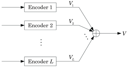
Figure 1: The overall subspace code as a superposition coding scheme.

Based on the definition (9) and (10), we further have the following property.

Property 2: For any two codewords of $\mathcal{C}$, $V=V_{1}\oplus\cdots\oplus V_{L}\,\,(V_{l}\in\mathcal{C}_{l})$ and $V^{{}^{\prime}}=V_{1}^{{}^{\prime}}\oplus\cdots\oplus V_{L}^{{}^{\prime}}\,\,(V_{l}^{{}^{\prime}}\in\mathcal{C}_{l}^{{}^{\prime}})$, $V=V^{{}^{\prime}}$ if and only if $V_{l}=V_{l}^{{}^{\prime}}$ for all $l$.

For the minimum distances of $\mathcal{C}$ and $\mathcal{C}_{l}$, the following property holds. For the proof, see [6].

Property 3: $d_{S}(\mathcal{C})=\min\big{\{}d_{S}(\mathcal{C}_{1}),d_{S}(\mathcal{C}_{2}),\cdots,d_{S}(\mathcal{C}_{L})\big{\}}$.

III-B Decoding algorithm I

Suppose that a codeword $V\in\mathcal{C}$ was transmitted and the vector space $U$ is now received. Corresponding to each $V_{l}\subseteq V$, we define a subspace $U_{l}\subseteq U$ as follows. It consists of all vectors of $U$ such that the elements at the coordinates $\big{\{}1,\cdots,\sum_{i=1}^{l-1}{n_{i}}\big{\}}\cup\big{\{}\sum_{i=1}^{l}{n_{i}+1,\cdots,\sum_{i=1}^{L}n_{i}}\big{\}}$ are zero. Now, we can describe decoding algorithm I as follows:

1. Extract $U_{l}$ from $U$;

2. Use the decoder for $\mathcal{C}_{l}$ to recover $V_{l}$ from $U_{l}$ [4], [5].

Note that given a set of vectors that span $U$, a basis of $U_{l}$ can be extracted with the aid of Gauss-Jordan elimination. Based on Property 2, once $V_{l}\in\mathcal{C}_{l}$ for all $l$ can be recovered, the transmitted codeword $V\in\mathcal{C}$ can be determined as $V=V_{1}\oplus\cdots\oplus V_{L}$.

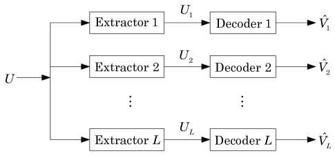
Figure 2: The schematic diagram of decoding algorithm I.

An illustration of the decoding algorithm is given in Fig. 2. It is seen that a parallel implementation is allowed. Moreover, if a receiver is only interested in a particular $V_{l}$, then he only needs to perform the corresponding layer in Fig. 2.

We now focus on the error-correction ability of decoding algorithm I. We first need to introduce a general result.

Lemma 1: Let $A$ and $B$ be two subspaces of $W$. Let $A^{{}^{\prime}}$ be a subspace of $A$. Then,

$$\textrm{dim}(A)-\textrm{dim}(A\cap B)\geqslant\textrm{dim}(A^{{}^{\prime}})-\textrm{dim}(A^{{}^{\prime}}\cap B).$$ (17)

Proof: Since $A\cap B$ is a subspace of $A$, there exists a (not unique) subspace $C$ of $A$ such that $A=(A\cap B)\oplus C$. Similarly, there exists a (not unique) subspace $D$ of $A^{{}^{\prime}}$ such that $A^{{}^{\prime}}=(A^{{}^{\prime}}\cap B)\oplus D$. Therefore, we only need to prove $\textrm{dim}(C)\geqslant\textrm{dim}(D)$.

Assume that there exists an $x\neq 0\in D\cap(A\cap B)$. Then $x\in D$ and $x\in B$. Since $A^{{}^{\prime}}=(A^{{}^{\prime}}\cap B)\oplus D$, we have $x\in A^{{}^{\prime}}$. So $x\in A^{{}^{\prime}}\cap B$, which together with $x\in D$ contradicts the fact $(A^{{}^{\prime}}\cap B)\cap D=\{0\}$. Therefore, $D\cap(A\cap B)=\{0\}$. Since $A^{{}^{\prime}}$ is a subspace of $A$ (by hypothesis) and $A^{{}^{\prime}}=(A^{{}^{\prime}}\cap B)\oplus D$, $D$ is a subspace of $A$. So $(A\cap B)\oplus D$ is a subspace of $A=(A\cap B)\oplus C$. Therefore, $\textrm{dim}(C)\geqslant\textrm{dim}(D)$, and the statement of the lemma follows.                                                                                                $\square$

For decoding algorithm I, we have the following result.

Theorem 2: $d_{S}(U,V)\geqslant d_{S}(U_{l},V_{l})$ for all $l$.

Proof: It is important to note that

$$V_{l}\cap U=V_{l}\cap U_{l}$$ (18)

and

$$U_{l}\cap V=U_{l}\cap V_{l}.$$ (19)

Then, based on Lemma 1, we have

$$\textrm{dim}(V)-\textrm{dim}(V\cap U)\geqslant\textrm{dim}(V_{l})-\textrm{dim}(V_{l}\cap U_{l})$$ (20)

and

$$\textrm{dim}(U)-\textrm{dim}(U\cap V)\geqslant\textrm{dim}(U_{l})-\textrm{dim}(U_{l}\cap V_{l}).$$ (21)

Summing up (14) and (15), we obtain

$$\textrm{dim}(V)+\textrm{dim}(U)-2\textrm{dim}(U\cap V)\geqslant\textrm{dim}(V_{l})+\textrm{dim}(U_{l})-2\textrm{dim}(U_{l}\cap V_{l}).$$ (22)

By the definition of subspace distance, $d_{S}(V,U)\geqslant d_{S}(V_{l},U_{l})$.                                                      $\square$

Combining Property 3 and Theorem 2, we have

Corollary 3: If $2d_{S}(V,U)<d_{S}(\mathcal{C})$, then $2d_{S}(V_{l},U_{l})<d_{S}(\mathcal{C}_{l})$ for all $l$.

The corollary indicates that decoding algorithm I is guaranteed to decode up to the error-correction capability of the overall code.

Note that it may happen that $2d_{S}(V,U)\geqslant d_{S}(\mathcal{C})$ while $2d_{S}(V_{l},U_{l})<d_{S}(\mathcal{C}_{l})$. In this case, the decoding algorithm can decode beyond the error-correction capability of the overall code. We give an example to show this.

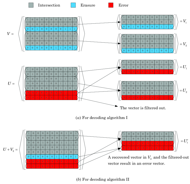
Figure 3: A transmitted codeword $V\in\mathcal{C}$ and the corresponding received $U$.

Example 1: Let the overall code $\mathcal{C}$ be composed of two component codes $\mathcal{C}_{1}$ and $\mathcal{C}_{2}$, which have parameters $n_{1}=3$, $n_{2}=4$, $m=4$, $d_{S}(\mathcal{C}_{1})=6$ and $d_{S}(\mathcal{C}_{2})=8$. According to Property 3, we have $d_{S}(\mathcal{C})=6$. Fig. 3 (a) gives a transmitted codeword $V\in\mathcal{C}$ and the corresponding received vector space $U$. Also shown in the figure are $V_{1}\in\mathcal{C}_{1}$, $V_{2}\in\mathcal{C}_{2}$, and $U_{1}$ and $U_{2}$ extracted from $U$. We note that in extracting $U_{1}$ and $U_{2}$, the vector of $U$ in the last row is filtered out.

It is easily verified that $d_{S}(V,U)=7+7-2\times 5=4$, $d_{s}(V_{1},U_{1})=3+3-2\times 2=2$, and $d_{S}(V_{2},U_{2})=4+4-2\times 3=2$. Consequently, we have $2d_{S}(V,U)>d_{S}(\mathcal{C})$, $2d_{S}(V_{1},U_{1})<d_{S}(\mathcal{C}_{1})$, and $2d_{S}(V_{2},U_{2})<d_{S}(\mathcal{C}_{2})$. Therefore, for the instantiated $V$ and $U$, decoding algorithm I decodes beyond the error-correction capability of the overall code.                                                                                                     $\square$

III-C Decoding algorithm II

It is well-known that for conventional superposition coding, the (iterative) successive interference cancellation (SIC) decoding algorithm is usually adopted [10]. Viewing a layered subspace code as a superposition coding scheme, we develop a SIC-like decoding algorithm, which is shown in Fig. 4. With a slight abuse of notation, the ‘$\oplus$’ here denotes the sum of two vector spaces that do not necessarily intersect trivially. By taking the dashed arrows into account, we obtain an iterative version of the algorithm. When decoder $l$ does not decode into a codeword of $\mathcal{C}_{l}$ (this can be checked by the decoder), we set $\hat{V}_{l}$ to be the zero subspace. So if there only occur erasures in the operator channel, the iterative version in general outperforms its non-iterative counterpart.

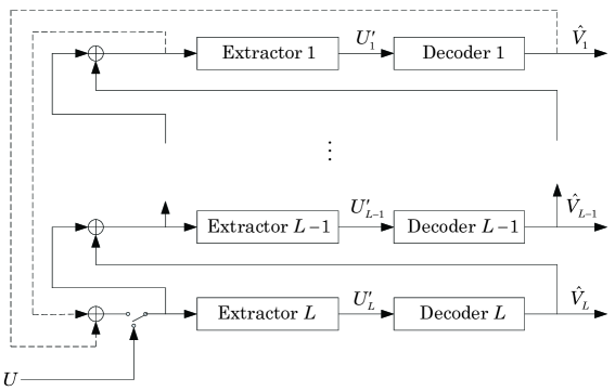
Figure 4: The schematic diagram of decoding algorithm II (dashed arrows for the iterative version).

It should be pointed out that in [8], the authors have used the idea of SIC to decode their constructed subspace codes. However, they did not mention any iterative decoding.

On the error-correction ability of decoding algorithm II, we have the following result.

Theorem 4: If $2d_{S}(V,U)<d_{S}(\mathcal{C})$, then $d_{S}(V,U)\geqslant d_{S}(V,U+\hat{V}_{L})\geqslant\cdots\geqslant d_{S}(V,U+\hat{V}_{L}+\cdots+\hat{V}_{1})$.

Proof: We prove the theorem by induction on $l$. Since $2d_{S}(V,U)<d_{S}(\mathcal{C})$, from Corollary 3, we have $\hat{V}_{l}=V_{l}\subseteq V$. Therefore, $\textrm{dim}(V+U)=\textrm{dim}\big{(}V+(U+\hat{V}_{l})\big{)}$ and $\textrm{dim}(V\cap U)\leqslant\textrm{dim}\big{(}V\cap(U+\hat{V}_{l})\big{)}$. Based on the definition of subspace distance, we have $d_{S}(V,U)\geqslant d_{S}(V,U+\hat{V}_{L})$.

Assume that $d_{S}(V,U)\geqslant d_{S}(V,U+\hat{V}_{L})\geqslant\cdots\geqslant d_{S}(V,U+\hat{V}_{L}+\cdots+\hat{V}_{l})$ holds. Since $2d_{S}(V,U)<d_{S}(\mathcal{C})$, $2d_{S}(V,U+\hat{V}_{L}+\cdots+\hat{V}_{l})<d_{S}(\mathcal{C})$. From Fig. 4, we see that $U+\hat{V}_{L}+\cdots+\hat{V}_{l}$ is the input to the extractor $l-1$. Based on Corollary 3, we have $\hat{V}_{l-1}=V_{l-1}\subseteq V$. Consequently, $d_{S}(V,U+\hat{V}_{L}+\cdots+\hat{V}_{l})\geqslant d_{S}(V,U+\hat{V}_{L}+\cdots+\hat{V}_{l-1})$. Thereby, the proof is complete.                                                          $\square$

From the proving process, we see that decoding algorithm II is guaranteed to decode up to the error-correction capability of the overall code.

Like decoding algorithm I, decoding algorithm II also occasionally decodes beyond the error-correction capability of the overall code. We note that the two algorithms may correct different errors in this case. We show this through the following example.

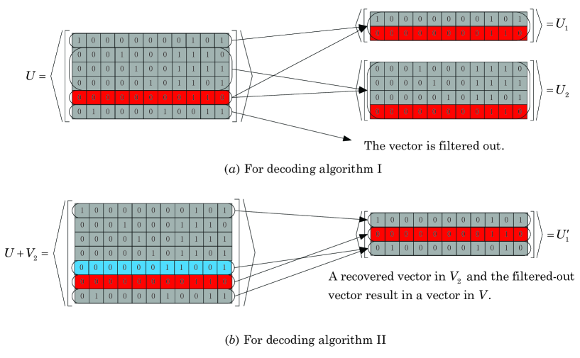
Figure 5: Decoding for another received $U$.

Example 2: For the parameters given in Example 1, we now use decoding algorithm II. Since $U_{2}^{{}^{\prime}}=U_{2}$, $V_{2}$ can be recovered. The resulting $U+V_{2}$ and $U_{1}^{{}^{\prime}}$ is shown in Fig. 3 (b). It is easily obtained that $d_{S}(V_{1},U_{1}^{{}^{\prime}})=3+4-2\times 2=3$. Since $2d_{S}(V_{1},U_{1}^{{}^{\prime}})=d_{S}(\mathcal{C}_{1})$, $V_{1}$ cannot be recovered with decoding algorithm II.

Consider again the transmitted $V$ in Example 1, but now suppose that the received $U$ is given as in Fig. 5. It is easily verified that $d_{S}(V,U)=7+6-2\times 5=3$, $d_{S}(V_{1},U_{1})=3+2-2\times 1=3$, and $d_{S}(V_{2},U_{2})=4+4-2\times 3=2$. Therefore, with decoding algorithm I, only $V_{2}$ can be recovered.

From the recovered $V_{2}$, we calculate $U+V_{2}$ and $U_{1}^{{}^{\prime}}$ as in Fig. 5 (b). Since $d_{S}(V_{1},U_{1}^{{}^{\prime}})=3+3-2\times 2=2$, we have $2d_{S}(V_{1},U_{1}^{{}^{\prime}})<d_{S}(\mathcal{C})$. So $V_{1}$ can be recovered with decoding algorithm II.

In summary, for the transmitted $V$ and the received $U$ in Fig. 3, only decoding algorithm I can correctly decode, while for the same $V$ and another $U$ as given in Fig. 5, only decoding algorithm II can correctly decode.                                                                                                                                 $\square$

IV Applications

In this section, we show that layered subspace codes can be applied in various scenarios for network coding.

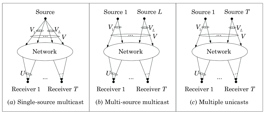
Figure 6: Possible application scenarios of layered subspace codes.

• Single-source multicast

  In this scenario, a single source communicates its information over a network to a specified set of $T$ receivers, as shown in Fig. 6 (a). The source is encoded with the overall subspace code and the basis vectors defining a codeword $V\in\mathcal{C}$ in (9) are transmitted. To deal with network dynamics, the number of component codes can be adapted. Therefore, this leads to an adaptive transmission scheme. On the other hand, by using component codes with different error-correction capabilities, the coding scheme can be used for unequal protection transmission [9].

• Multi-source multicast [7]

  As shown in Fig. 6 (b), $L$ sources transmit independent information over a network to a specified set of $T$ receivers. Source $l$ is encoded with component code $l$ and the basis vectors defining a codeword $V_{l}\in\mathcal{C}_{l}$ in (10) are transmitted. Based on the received vectors, each receiver tries to recover $V_{l}$ for all $l$.

• Multiple unicasts

  A unicast means that a single source communicates its information over a network to a single receiver. In the multiple unicasts scenario, the number of receivers is equal to that of sources, as shown in Fig. 6 (c), and receiver $l$ only requests the information from source $l$. The coding scheme is the same as in the multi-source multicast scenario. Since receiver $l$ only wishes to recover $V_{l}$, decoding algorithm I is preferred in this scenario.

V Conclusion

We treated the layered subspace codes in [7] as a superposition coding scheme and proposed two efficient decoding algorithms. Error-correction abilities of both algorithms are analyzed. As an error control scheme, layered subspace codes can be expected to find various applications for network coding.

References

- [1] R. Ahlswede, N. Cai, S.-Y. R. Li, and R. W. Yeung, “Network information flow,” IEEE Trans. Inform. Theory, vol. 46, no. 6, pp. 1204-1216, Jul. 2000.
- [2] T. Ho, M. Medard, R. Kötter, D. R, Karger, M. Effros, J. Shi, and B. Leong, “A random linear network coding approach to multicast,” IEEE Trans. Inform. Theory, vol. 52, no. 10, pp. 4413-4430, Oct. 2006.
- [3] N. Cai and R. W. Yeung, “Network coding and error correction,” in Proc. IEEE Info. Theory Workshop, Bangalore, India, October 2002, pp. 20-25.
- [4] R. Kötter and F. R. Kschischang, “Coding for errors and erasures in random network coding,” IEEE Trans. Inform. Theory, vol. 54, no. 8, pp. 3579-3591, Aug. 2008.
- [5] D. Silva, F. R. Kschischang and R. Kötter, “A rank-metric approach to error control in random network coding,” IEEE Trans. Inform. Theory, vol. 54, no. 9, pp. 3951-3967, Sept. 2008.
- [6] E. M. Gabidulin, “Theorey of codes with maximum rank distance,” Probl. Inform. Transmission, vol. 21, no. 1, pp. 3-16, Jan. 1985.
- [7] M. J. Siavoshani, C. Fragouli, and S. Diggavi, “Code construction for multiple sources network coding,” in MobiHoc 2009, pp. 21-24.
- [8] T. Dikaliotis, T. Ho, S. Jaggi, S. Vyetrenko, H. Yao, M. Effors, J. Kliewer, and E. Erez, “Multiple-access network information-flow and correction codes,” IEEE Trans. Inform. Theory, vol. 57, no. 2, pp. 1067-1079, Feb. 2011.
- [9] Z. Yan and B. W. Suter, “Unequal error protection for noncoherent random linear network coding,” in Proc. CISS, 2011, pp. 1-6.
- [10] R. Zhang and L. Hanzo, “A unified treatment of superposition coding aided communications: theory and practice,” IEEE Communications Surveys & Tutorials, vol. 13, no. 3, Third Quarter, 2011.
- [11] P. R. Halmos. Finite-dimensional vector spaces, Berlin, New York: Springer-Verlag, 1974.