Operator Product Expansion with analytic QCD in $\tau$ decay physics

Abstract

We apply a recently constructed model of analytic QCD in the Operator Product Expansion (OPE) analysis of the $\tau$ lepton decay data in the $V$+$A$ channel. The model has the running coupling ${\mathcal{A}}_{1}(Q^{2})$ with no unphysical singularities, i.e., it is analytic. It differs from the corresponding perturbative QCD coupling $a(Q^{2})$ at high squared momenta $|Q^{2}|$ by terms $\propto(1/Q^{2})^{5}$, hence it does not contradict the ITEP OPE philosophy and can be consistently applied with OPE up to terms of dimension $D=8$. In evaluations for the Adler function we use a Padé-related renormalization-scale-independent resummation, applicable in any analytic QCD model. Applying the Borel sum rules in the $Q^{2}$ plane along rays of the complex Borel scale and comparing with ALEPH data of 1998, we obtain the gluon condensate value $\langle(\alpha_{s}/\pi)G^{2}\rangle=0.0055\pm 0.0047\ {\rm GeV}^{4}$. Consideration of the $D=6$ term gives us the result $\langle O_{6}^{(V+A)}\rangle=(-0.5\pm 1.1)\times 10^{-3}\ {\rm GeV}^{6}$, not incompatible with nonnegative values. The real Borel transform gives us then, for the central values of the two condensates, a good agreement with the experimental results in the entire considered interval of the Borel scales $M^{2}$. In perturbative QCD in $\overline{\rm MS}$ scheme we deduce similar result for the gluon condensate, $0.0059\pm 0.0049\ {\rm GeV}^{4}$, but the value of $D=6$ condensate is negative, $\langle O_{6}^{(V+A)}\rangle=(-1.8\pm 0.9)\times 10^{-3}\ {\rm GeV}^{6}$, and the resulting real Borel transform for the central values is close to the lower bound of the experimental band.

I Introduction

Perturbative QCD (pQCD) in the usual renormalization schemes, such as $\overline{\rm MS}$, has the peculiar property of resulting in a running coupling $a(Q^{2})$ ($\equiv\alpha_{s}(Q^{2})/\pi$) which has singularities in the complex $Q^{2}$ plane outside of the negative semiaxis, often at positive $Q^{2}\equiv-q^{2}>0$. This implies that spacelike physical quantities ${\cal D}(Q^{2})$ evaluated in terms of $a(Q^{2})$ have the same type of singularities, contravening the general principles of (causal and local) quantum field theories BS ; Oehme . These problematic aspects of pQCD were addressed in the seminal works of Shirkov, Solovtsov et al. ShS ; MSS ; Sh who constructed, as an alternative, a QCD model which has no such unphysical singularities. Their idea was to keep the discontinuity function $\rho_{1}^{\rm(pt)}(\sigma)={\rm Im}\ a(-\sigma-i\epsilon)$ unchanged for $Q^{2}\leq 0$ ($\sigma\geq 0$), but eliminating the offending singularities at $Q^{2}>0$ by not including them in the dispersion relation for their coupling. The same principle was applied to any other integer power of $a(Q^{2})$. This approach was called Analytic Perturbation Theory (APT); in the present context we call it Minimal Analytic (MA) QCD, due to the unchanged (perturbative) singularities along the $Q^{2}\leq 0$ semiaxis. For various applications of MA and related models, see Refs. Sh ; MSSY ; Milton:2001mq ; mes2 ; Pase ; NesSim ; Bdecays ; rev1 ; rev2 ; rev3 . However, MA has two aspects which, under specific circumstances, may be regarded as inconvenient:

1. It subestimates MSS ; MSSY the semihadronic $\tau$ decay ratio $r_{\tau}$, giving $r_{\tau}({\rm MA})\approx 0.13$-$0.14$ in the strangeless $V$+$A$ channel while the experimental value is $0.203\pm 0.004$ ALEPH2 ; DDHMZ .

2. At momenta $Q^{2}>\Lambda^{2}$ (where $\Lambda^{2}\sim 0.1\ {\rm GeV}^{2}$), the MA coupling ${\mathcal{A}}_{1}^{\rm(MA)}(Q^{2})$ differs from the underlying QCD coupling $a(Q^{2})$ by terms $\sim(\Lambda^{2}/Q^{2})$. The latter property implies that, in MA, the leading-twist contributions to physical quantities contain power terms $\sim(\Lambda^{2}/Q^{2})$ which are of ultraviolet origin. This is not in accordance with the ITEP interpretation of OPE Shifman:1978bx ; DMW which states that the higher-dimension (higher-twist) terms $\sim(\Lambda^{2}/Q^{2})^{n}$ in OPE are of infrared origin.

These problems have been addressed in a series of papers panQCD ; 1danQCD ; 2danQCD . In Ref. panQCD the following question was investigated: Is there an analytic QCD which is simultaneously fully perturbative and reproduces the correct value of $r_{\tau}$? The results of Ref. panQCD indicate that there is probably no such framework, unless we introduce renormalization schemes which make the perturbation series highly divergent starting at terms $\sim a^{5}$. Therefore, in Refs. 1danQCD ; 2danQCD a more modest goal was pursued: construction of analytic QCD which is not fully perturbative, but addresses the previously mentioned two points nonetheless: the correct value of $r_{\tau}$ is reproduced, and the deviation of the analytic coupling ${\mathcal{A}}_{1}(Q^{2})$ from the underlying perturbative coupling $a(Q^{2})$ at high $|Q^{2}|$ is proportional to a “sufficiently high” power of $1/Q^{2}$. In Ref. 1danQCD , an analytic model was constructed for which ${\mathcal{A}}_{1}(Q^{2})-a(Q^{2})\sim(\Lambda^{2}/Q^{2})^{3}$ at high $|Q^{2}|>\Lambda^{2}$. This was achieved by constructing the model-defining discontinuity function $\rho_{1}(\sigma)\equiv{\rm Im}\ {\mathcal{A}}_{1}(-\sigma-i\epsilon)$ in such a way that it is equal to the discontinuity function $\rho_{1}^{\rm(pt)}(\sigma)\equiv{\rm Im}\ a(-\sigma-i\epsilon)$ of the underlying pQCD coupling $a(Q^{2})$ at $\sigma>M_{0}^{2}$ (where $M_{0}\sim 1$ GeV), and in the low-$\sigma$ regime $(0<\sigma<M_{0}^{2})$ the unknown behavior of $\rho_{1}(\sigma)$ was parametrized by a single delta function. By adjusting the free parameters of the model, the aforementioned suppressed deviation ${\mathcal{A}}_{1}(Q^{2})-a(Q^{2})\sim(\Lambda^{2}/Q^{2})^{3}$ at $Q^{2}>\Lambda^{2}$ was achieved. In Ref. 2danQCD , this idea was continued, by employing in the low-energy regime ($0<\sigma<M_{0}^{2}$) the parametrization in terms of two delta functions for the discontinuity function $\rho_{1}(\sigma)$. In this way, the strongly suppressed deviation ${\mathcal{A}}_{1}(Q^{2})-a(Q^{2})\sim(\Lambda^{2}/Q^{2})^{5}$ at $Q^{2}>\Lambda^{2}$ was achieved (while at the same time the correct value of $r_{\tau}$ was reproduced). Therefore, in this model the leading-twist contributions to physical quantities do not give power-suppressed terms of dimension $D<10$ of ultraviolet origin. Hence, the model can be applied with OPE, without contradicting the ITEP interpretation of OPE, up to $D=8$ terms.

We wish to point out that our approach eliminates unphysical singularities from the QCD coupling while still preserving the salient features of the usual pQCD approach, among them the applicability of OPE (in the ITEP sense) and the related universality of the QCD coupling. On the other hand, the approaches of Refs. Milton:2001mq ; mes2 ; Nest3 ; DeRafael ; MagrDual follow a different line: by considering (various) specific timelike observables, they eliminate the unphysical singularities directly from the corresponding spacelike observables. This leads either directly Milton:2001mq ; mes2 ; Nest3 or indirectly DeRafael ; MagrDual to analytic QCD couplings whose nonunversality is reflected in observable-dependent modifications in the low-energy (low-$\sigma$) regime.

In this work, we will apply the mentioned analytic model of Ref. 2danQCD to the analysis of the $\tau$-decay data, in the $V$+$A$ channel, using the OPE approach (with up to $D=6$ terms) with Borel sum rules, along the lines of Refs. Geshkenbein ; Ioffe where the analysis was performed within the perturbative QCD in $\overline{\rm MS}$ scheme. The program of the work is the following. In Sec. II we summarize the previously mentioned QCD analytic model 2danQCD . In Sec. III we recapitulate a powerful Padé-related resummation method BGA which is very natural and convenient to apply in evaluations of physical quantities within analytic QCD models. In Sec. IV we apply this resummation, within our model, in the evaluation of the (leading-dimension part of the) Adler function, i.e., the logarithmic derivative of the polarization operator $\Pi(Q^{2})$ in the massless limit. We combine this evaluation, and the OPE expansion of the Adler function, with the Borel sum rules along rays in the complex plane of the Borel scales $M^{2}$ (as in Refs. Geshkenbein ; Ioffe ; cf. also. Ref. Ioffe:2000ns ). For the experimental input we use ALEPH results of 1998 for $\omega_{\rm exp}(\sigma)$ ($\propto{\rm Im}\ \Pi(-\sigma-i\epsilon)$) obtained from $\tau$-decay invariant-mass spectra for $0<\sigma<m_{\tau}^{2}$ ALEPH1 . We also discuss the obtained results and compare them with the results obtained when no resummation is performed in analytic QCD, and with the results in perturbative QCD in the renormalization scheme that is underlying the analytic QCD model (with and without resummation) and in $\overline{\rm MS}$ renormalization scheme. Section V contains a summary of the obtained results and conclusions.

II 2-delta analytic QCD

Here we recapitulate the analytic QCD model of Ref. 2danQCD , which contains a parametrization with two delta functions in the low-$\sigma$ regime of the discontinuity function $\rho_{1}(\sigma)={\rm Im}\ {\mathcal{A}}_{1}(-\sigma-i\epsilon)$. Any analytic QCD model is defined, in principle, via its analytic spacelike coupling ${\mathcal{A}}_{1}(Q^{2})$, which is the analytic analog of the perturbative coupling $a(Q^{2})\equiv\alpha_{s}(Q^{2})/\pi$. Any other coupling ${\mathcal{A}}_{n}(Q^{2})$ (analog of the power $a(Q^{2})^{n}$) can then be constructed from it, via the formalism introduced in Refs. GCCV when $n$ is integer and in Ref. GCAK when $n$ is general noninteger. On the other hand, the coupling ${\mathcal{A}}_{1}(Q^{2})$, analytic in the complex plane outside of the negative semiaxis $Q^{2}\in\mathbb{C}\backslash(-\infty,0]$, can be expressed via the discontinuity function $\rho_{1}(\sigma)\equiv{\rm Im}\ {\mathcal{A}}_{1}(-\sigma-i\epsilon)$ which is defined only for $\sigma>0$. The expression is a dispersion relation which follows from the application of the Cauchy theorem, the analyticity of ${\mathcal{A}}_{1}(Q^{2})$, and the asymptotic freedom at large $|Q^{2}|$

$${\mathcal{A}}_{1}(Q^{2})=\frac{1}{\pi}\int_{0}^{+\infty}\ d\sigma\frac{\rho_{1}(\sigma)}{(\sigma+Q^{2})}\ .$$ (1)

Due to the success of perturbative QCD at high energies, it is reasonable to assume that at higher $\sigma$ ($\sigma>M_{0}^{2}$, where $M_{0}\gtrsim 1$ GeV) the discontinuity function $\rho_{1}(\sigma)$ coincides with the underlying perturbative function $\rho_{1}^{\rm(pt)}(\sigma)\equiv{\rm Im}\ a(-\sigma-i\epsilon)$. In the low-$\sigma$ regime ($0<\sigma<M_{0}^{2}$) the behavior is unknown in its details, and is here parametrized with two delta functions at lower values $\sigma=M_{1}^{2}$ and $M_{2}^{2}$ ($0<M_{2}^{2}<M_{1}^{2}<M_{0}^{2}$)

$$\rho_{1}^{\rm(2\delta)}(\sigma;c_{2}) = \pi\sum_{j=1}^{2}f_{j}^{2}\Lambda^{2}\;\delta(\sigma-M_{j}^{2})+\Theta(\sigma-M_{0}^{2})\times\rho_{1}^{\rm(pt)}(\sigma;c_{2})$$ (2)

$$= \pi\sum_{j=1}^{2}f_{j}^{2}\;\delta(s-s_{j})+\Theta(s-s_{0})\times r_{1}^{\rm(pt)}(s;c_{2})\ .$$ (3)

In Eq. (3) dimensionless parameters were introduced: $s=\sigma/\Lambda^{2}$, $s_{j}=M_{j}^{2}/\Lambda^{2}$ ($j=0,1,2$), and $r_{1}^{\rm(pt)}(s;c_{2})=\rho_{1}^{\rm(pt)}(\sigma;c_{2})={\rm Im}\ a(Q^{2}=-\sigma-i\epsilon;c_{2})$, $c_{2}$ being a scheme parameter. The Lambert scale $\Lambda^{2}$ ($\stackrel{{\scriptstyle<}}{{\sim}}10^{-1}\ {\rm GeV}^{2}$) will be defined below. The underlying perturbative coupling $a(Q^{2})$ is taken, for convenience, in such renormalization schemes where it can be expressed explicitly as a solution in terms of the Lambert function $W(z)$

$$a(Q^{2};c_{2})=-\frac{1}{c_{1}}\frac{1}{\left[1-c_{2}/c_{1}^{2}+W_{\mp 1}(z)\right]}\ .$$ (4)

Here, $Q^{2}=|Q^{2}|\exp(i\phi)$; $W_{-1}$ and $W_{+1}$ are the branches of the Lambert function for $0\leq\phi<+\pi$ and $-\pi<\phi<0$, respectively, and the variable $z$ involves the mentioned Lambert scale $\Lambda$

$$z=-\frac{1}{c_{1}e}\left(\frac{|Q^{2}|}{\Lambda^{2}}\right)^{-\beta_{0}/c_{1}}\exp\left(-i{\beta_{0}}\phi/c_{1}\right)\ .$$ (5)

The explicit expression (4) was presented in Ref. Gardi:1998qr . It is the solution of the following (perturbative) renormalization group equation (RGE):

$$\frac{\partial a(Q^{2};c_{2})}{\partial\ln Q^{2}} = -\beta_{0}a^{2}\frac{\left[1+(c_{1}-(c_{2}/c_{1}))a\right]}{\left[1-(c_{2}/c_{1})a\right]}\ .$$ (6)

Here, $\beta_{0}=(1/4)(11-2n_{f}/3)$ and $c_{1}=\beta_{1}/\beta_{0}=(1/4)(102-38n_{f}/3)/(11-2n_{f}/3)$ are universal constants. On the other hand, $c_{2}\equiv\beta_{2}/\beta_{0}$ is the free three-loop renormalization scheme parameter. The expansion of the above beta function $\beta(a)=\partial a/\partial\ln Q^{2}$ gives

$$\beta(a)=-\beta_{0}a^{2}(1+c_{1}a+c_{2}a^{2}+c_{3}a^{3}+\ldots)\ ,$$ (7)

with the higher renormalization scheme parameters $c_{j}\equiv\beta_{j}/\beta_{0}$ ($j\geq 3$) fixed by the value of $c_{2}$: $c_{j}=c_{2}^{j-1}/c_{1}^{j-2}$ ($j\geq 3$).

Application of the dispersion relation (1) to the discontinuity function (3) gives the analytic coupling ${\mathcal{A}}_{1}(Q^{2})$ of the model

$${\mathcal{A}}_{1}(Q^{2};c_{2})=\sum_{j=1}^{2}\frac{f_{j}^{2}}{(u+s_{j})}+\frac{1}{\pi}\int_{s_{0}}^{\infty}ds\;\frac{r_{1}^{\rm(pt)}(s;c_{2})}{(s+u)}\ ,$$ (8)

where $u=Q^{2}/\Lambda^{2}$. The free parameters of the model ($c_{2}$, $\Lambda$, $s_{0}$, $s_{1}$, $f_{1}^{2}$, $s_{2}$, $f_{2}^{2}$) are fixed by various requirements. The scale $\Lambda$ is fixed by requiring that the underlying perturbative coupling $a(Q^{2})$ reproduce the central value of the world average at $Q^{2}=M_{Z}^{2}$ as given in Ref. PDG2010 : $a^{({\overline{\rm MS}})}(M_{Z}^{2})=0.1184/\pi$. More specifically, the coupling $a(Q^{2};c_{2})$, with a chosen value of $c_{2}$ and in the considered low-momentum regime of interest ($Q<2{\overline{m}}_{c}$ where $n_{f}=3$), is first transformed to the exact four-loop $\overline{\rm MS}$ scheme, then RGE-evolved up to $Q^{2}=M_{Z}^{2}$ using the four-loop $\overline{\rm MS}$ beta function and at the quark thresholds $Q^{2}_{\rm thr}=(2{\overline{m}}_{q})^{2}$ using the three-loop matching conditions CKS . The Lambert scale $\Lambda$ (at $n_{f}=3$) is then fixed such that the described procedure leads to the value $a^{({\overline{\rm MS}})}(M_{Z}^{2})=0.1184/\pi$. The four parameters $s_{j}$ and $f_{j}^{2}$ ($j=1,2$), at chosen values of $s_{0}$ and $c_{2}$, are determined as functions of $s_{0}$ by the earlier mentioned (ITEP-OPE motivated) requirement ${\mathcal{A}}_{1}(Q^{2})-a(Q^{2})\sim(\Lambda^{2}/Q^{2})^{5}$ for $|Q^{2}|>\Lambda^{2}$ (these are four requirements, in fact). Subsequently, the value of the parameter $s_{0}$ ($\equiv M_{0}^{2}/\Lambda^{2}$) is determined, for a chosen value of $c_{2}$, by the requirement that the model reproduce the aforementioned experimental value of the $V$+$A$ strangeless semihadronic $\tau$ decay ratio $r_{\tau}\approx 0.203$. Finally, the values of the parameter $c_{2}$ are varied in such a way that the resulting pQCD-onset scale $M_{0}$ ($\sim 1$ GeV) varies within a specific range. For phenomenological reasons, the preferred values of $M_{0}$ should be below and not too close to the value of the $\tau$ lepton mass ($m_{\tau}=1.777$ GeV). On the other hand, if $M_{0}<1.15$ GeV, the values of ${\mathcal{A}}_{1}(Q^{2})$ become too large (${\mathcal{A}}_{1}(0)>1$) and the model loses stability in the infrared. We choose the representative values of the scheme parameter $c_{2}$ such that the following conditions are fulfilled: $1\ {\rm GeV}<M_{0}<1.5\ {\rm GeV}$ and ${\mathcal{A}}_{1}(0)\leq 1$. For the central value $M_{0}=1.25$ GeV, we have the values of parameters given in the second line of Table 1. The two border choices ($M_{0}=1$ GeV; and ${\mathcal{A}}_{1}(0)=1$ with $M_{0}\approx 1.15$ GeV) are also given in Table 1.

Table 1: Values of the parameters of the considered two-delta anQCD model, under the restriction for the values of the pQCD-onset scale $M_{0}\equiv\sqrt{s_{0}}\Lambda$: $1\ {\rm GeV}\leq M_{0}\leq 1.5\ {\rm GeV}$, and ${\mathcal{A}}_{1}(0)\leq 1.0$. The corresponding Lambert scales $\Lambda$ are for the central value of the QCD coupling parameter $\alpha_{s}^{({\overline{\rm MS}})}(M_{Z}^{2})=0.1184$.

$c_{2}=\beta_{2}/\beta_{0}$	$s_{0}$	$s_{1}$	$f_{1}^{2}$	$s_{2}$	$f_{2}^{2}$	$\Lambda$ [GeV]	$M_{0}$	${\mathcal{A}}_{1}(0)$
-5.73	25.01	18.220	0.3091	0.7082	0.6312	0.231	1.15	1.00
-4.76	23.06	16.837	0.2713	0.8077	0.5409	0.260	1.25	0.776
-2.10	17.09	12.523	0.1815	0.7796	0.3462	0.363	1.50	0.544

However, the world average of the coupling parameter PDG2010 has some uncertainty: $a^{({\overline{\rm MS}})}(M_{Z}^{2})=(0.1184\pm 0.0007)/\pi$, corresponding to $a^{({\overline{\rm MS}})}(m_{\tau}^{2})_{n_{f}=3}=(0.3183\pm 0.0057)/\pi$, i.e., ${\overline{\Lambda}}_{n_{f}=3}=0.336\pm 0.010$ GeV where ${\overline{\Lambda}}_{n_{f}=3}$ is the usual $\overline{\rm MS}$ scale (at $n_{f}=3$). This implies that the Lambert scale varies, $\Lambda\approx 0.260\pm 0.008$ GeV [$a(m_{\tau}^{2},c_{2})=(0.2905\pm 0.0043)/\pi$], while all the (central) values of the dimensionless parameters of the model ($c_{2}=-4.76,s_{0}=23.06$, etc.) are unchanged. The predicted value of the $V$+$A$ $\tau$-decay ratio then varies, $r_{\tau}=0.203\pm 0.006$, which is still compatible with the experimental value $0.203\pm 0.004$ ALEPH2 ; DDHMZ .

Having the analytic analog $(a(Q^{2}))_{\rm an}={\mathcal{A}}_{1}(Q^{2})$ in 2-delta QCD analytic model in Eq. (8), the analytization of higher integer powers $(a^{n})_{\rm an}={\mathcal{A}}_{n}$ is performed according to the construction in Refs. GCCV which is applicable to any analytic QCD model. We briefly present it below. The basic idea is to introduce the logarithmic derivatives

$${{\widetilde{a}}}_{n+1}(Q^{2})\equiv\frac{(-1)^{n}}{\beta_{0}^{n}n!}\frac{\partial^{n}a(Q^{2})}{\partial(\ln Q^{2})^{n}}\ ,\qquad(n=1,2,\ldots)\ .$$ (9)

We note that ${{\widetilde{a}}}_{n+1}(Q^{2})=a(Q^{2})^{n+1}+{\cal O}(a^{n+2})$ by RGE $\partial a(Q^{2})/\partial\ln Q^{2}=\beta(a(Q^{2}))$, where beta function $\beta(a)$ has the pQCD expansion as given in Eq. (7). Due to the linearity of analytization, it follows from $(a(Q^{2}))_{\rm an}={\mathcal{A}}_{1}(Q^{2})$ the relation $(\partial a(Q^{2})/\partial\ln Q^{2})_{\rm an}=\partial{\mathcal{A}}_{1}(Q^{2})/\partial\ln Q^{2}$, and thus in general

$$\left({{\widetilde{a}}}_{n+1}(Q^{2})\right)_{\rm an}={\widetilde{\mathcal{A}}}_{n+1}(Q^{2})\ ,$$ (10)

where

$${\widetilde{\mathcal{A}}}_{n+1}(Q^{2})\equiv\frac{(-1)^{n}}{\beta_{0}^{n}n!}\frac{\partial^{n}{\mathcal{A}}_{1}(Q^{2})}{\partial(\ln Q^{2})^{n}}\ .\qquad(n=1,2,\ldots)\ ,$$ (11)

and where ${\mathcal{A}}_{1}(Q^{2})$ is given in our case in Eq. (8). An interesting aspect is that in virtually any analytic QCD model, including the present one, we have a clear hierarchy $|{\mathcal{A}}_{1}(Q^{2})|>|{\widetilde{\mathcal{A}}}_{2}(Q^{2})|>|{\widetilde{\mathcal{A}}}_{3}(Q^{2})|>\cdots$ not just for large $|Q^{2}|>\Lambda^{2}$, but for any $Q^{2}$, cf. curves in Fig. 1(a) (which are for the presented model and at $Q^{2}>0$).

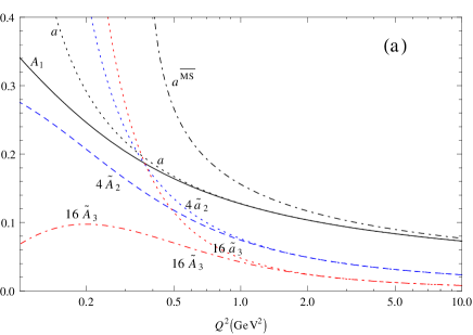
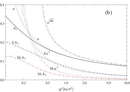
Figure 1: (a) The couplings ${\mathcal{A}}_{1}(Q^{2})$, $4\times{\widetilde{\mathcal{A}}}_{2}(Q^{2})$ and $4^{2}\times{\widetilde{\mathcal{A}}}_{3}(Q^{2})$ of 2-delta analytic QCD model with the central input values ($c_{2}=-4.76$; $s_{0}=23.06$), as a function of positive $Q^{2}$: $0.1\ {\rm GeV}^{2}\leq Q^{2}\leq 10.0\ {\rm GeV}^{2}$; the rescaling factors $4$ and $4^{2}$ are for better visibility; included are the analogous pQCD couplings $a$, $4\times{\widetilde{a}}_{2}$ and $4^{2}\times{\widetilde{a}}_{3}$ in the same (Lambert) scheme, and the $\overline{\rm MS}$ coupling $a^{\overline{\rm MS}}$. (b) The couplings ${\mathcal{A}}_{1}(Q^{2})$, $4\times{\mathcal{A}}_{2}(Q^{2})$ and $4^{2}\times{\mathcal{A}}_{3}(Q^{2})$, where the couplings ${\mathcal{A}}_{2}$ and ${\mathcal{A}}_{3}$ are constructed by Eqs. (22)-(23) with truncation at (including) ${\widetilde{\mathcal{A}}}_{4}$ term; included are the (Lambert) pQCD analogs $a$, $4a^{2}$ and $4^{2}a^{3}$.

This suggests the following approach to the evaluation of any dimension-zero ($D=0$) contribution ${\cal D}(Q^{2})$ of a massless spacelike observable, such as Adler function, in analytic QCD. Let the perturbation series (pt) of this quantity be

$${\cal D}(Q^{2})_{\rm pt} = a(\kappa Q^{2})\sum_{n=1}^{\infty}d_{n}(\kappa)\;a(\kappa Q^{2})^{n+1}\ ,$$ (12)

where $\mu^{2}=\kappa Q^{2}$ is a renormalization scale, $\kappa\sim 1$ being a fixed chosen dimensionless renormalization scale parameter. Before evaluating ${\cal D}(Q^{2})$ in analytic QCD, we reorganize the above series into the corresponding “modified” perturbation series (mpt) in logarithmic derivatives ${\widetilde{a}}_{n+1}$, Eq. (9)

$${\cal D}(Q^{2})_{\rm mpt} = a(\kappa Q^{2})+\sum_{n=1}^{\infty}{{\widetilde{d}}}_{n}(\kappa)\;{{\widetilde{a}}}_{n+1}(\kappa Q^{2})\ .$$ (13)

This leads, after applying the analytization (10) term-by-term, to the (“modified”) analytic series (man)

$${\cal D}(Q^{2})_{\rm man} = {\mathcal{A}}_{1}(\kappa Q^{2})+\sum_{n=1}^{\infty}{{\widetilde{d}}}_{n}(\kappa)\;{\widetilde{\mathcal{A}}}_{n+1}(\kappa Q^{2})\ ,$$ (14)

which is the basic expression for evaluation of ${\cal D}(Q^{2})$ in analytic QCD.

Since the “mpt” series (13) is just a reorganization of the $\kappa$-independent “pt” series (12), the “mpt” series ${\cal D}(Q^{2})_{\rm mpt}$ is also $\kappa$-independent. This then immediately implies, in conjunction with the recurrence relation $\partial{\widetilde{a}}_{n}(\kappa Q^{2})/\partial\ln\kappa=-\beta_{0}n{\widetilde{a}}_{n+1}(\kappa Q^{2})$ [this being a direct consequence of the definition (9)], the following set of differential relations between ${\widetilde{d}}_{n}(\kappa)$:

$$\frac{d}{d\ln\kappa}{\widetilde{d}}_{n}(\kappa)=n\beta_{0}{\widetilde{d}}_{n-1}(\kappa)\qquad(n=1,2,\ldots)\ ,$$ (15)

where $d_{0}(\kappa)={{\widetilde{d}}}_{0}(\kappa)=1$ by definition. Using these relations, it is straightforward to verify that the (“modified”) analytic series ${\cal D}(Q^{2})_{\rm man}$ of Eq. (14) is $\kappa$-independent.

The coefficients ${\widetilde{d}}_{n}(\kappa)$ are obtained from $d_{k}(\kappa)$’s ($k\leq n$) in the following way. We first relate powers $a^{n+1}$ and the logarithmic derivatives ${\widetilde{a}}_{n+1}$, at a given scale $Q^{2}$ (or: $\mu^{2}=\kappa Q^{2}$) using the RGE relations in pQCD

$${\widetilde{a}}_{2} = a^{2}+c_{1}a^{3}+c_{2}a^{4}+\cdots\ ,$$ (16)

$${\widetilde{a}}_{3} = a^{3}+\frac{5}{2}c_{1}a^{4}+\cdots\ ,\qquad{\widetilde{a}}_{4}=a^{4}+\cdots\ ,\qquad{\rm etc.}\ ,$$ (17)

and we invert them

$$a^{2} = {\widetilde{a}}_{2}-c_{1}{\widetilde{a}}_{3}+\left(\frac{5}{2}c_{1}^{2}-c_{2}\right){\tilde{a}}_{4}+\cdots\ ,$$ (18)

$$a^{3} = {\widetilde{a}}_{3}-\frac{5}{2}c_{1}{\widetilde{a}}_{4}+\cdots\ ,\qquad a^{4}={\widetilde{a}}_{4}+\cdots\ ,\qquad{\rm etc.}$$ (19)

Replacing the relations (18)-(19) into the perturbation expansion (12) for ${\cal D}(Q^{2})$ we can read off the tilde coefficients ${\widetilde{d}}_{n}(\kappa)$ of the reorganized (“modified”) expansions (13)-(14)

$${\widetilde{d}}_{1}(\kappa) = d_{1}(\kappa)\ ,\qquad{\widetilde{d}}_{2}(\kappa)=d_{2}(\kappa)-c_{1}d_{1}(\kappa)\ ,$$ (20)

$${\widetilde{d}}_{3}(\kappa) = d_{3}(\kappa)-\frac{5}{2}c_{1}d_{2}(\kappa)+\left(\frac{5}{2}c_{1}^{2}-c_{2}\right)d_{1}(\kappa)\ ,\qquad{\rm etc.}$$ (21)

Applying analytization, Eqs. (10)-(11), in relations (18)-(19) term-by-term, we finally obtain the analytic analogs of integer powers, ${\mathcal{A}}_{n}=(a^{n})_{\rm an}$

$${\mathcal{A}}_{2} \equiv \left(a^{2}\right)_{\rm an}={\widetilde{\mathcal{A}}}_{2}-c_{1}{\widetilde{\mathcal{A}}}_{3}+\left(\frac{5}{2}c_{1}^{2}-c_{2}\right){\widetilde{\mathcal{A}}}_{4}+\cdots\ ,$$ (22)

$${\mathcal{A}}_{3} \equiv \left(a^{3}\right)_{\rm an}={\widetilde{\mathcal{A}}}_{3}-\frac{5}{2}c_{1}{\widetilde{\mathcal{A}}}_{4}+\cdots\ ,\quad{\mathcal{A}}_{4}\equiv\left(a^{4}\right)_{\rm an}={\widetilde{\mathcal{A}}}_{4}+\cdots\ ,\qquad{\rm etc.}$$ (23)

This means that the “modified” analytic series (14) can be rewritten in the more usual form, in close analogy with the original perturbation series (12)

$${\cal D}(Q^{2})_{\rm an} = {\mathcal{A}}_{1}(\kappa Q^{2})+\sum_{n=1}^{\infty}d_{n}(\kappa)\;{\mathcal{A}}_{n+1}(\kappa Q^{2})\ .$$ (24)

This series, being a reorganization of the $\kappa$-independent series ${\cal D}(Q^{2})_{\rm man}$ of Eq. (14), is therefore also $\kappa$-independent. Several couplings ${\mathcal{A}}_{n}$ in the present analytic QCD model, for low positive $Q^{2}$, are presented in Fig. 1(b).

In practice, in the expansions of ${\cal D}(Q^{2})$, Eqs. (12) and (13), we know exactly only a few first coefficients $d_{n}(\kappa)$, up to (and including) $n=n_{\rm max}$, i.e., up to $a^{n_{\rm max}+1}$. This implies that in the relations (16)-(19) and (22)-(23) it is natural to perform truncations at (and including) the term $\sim a^{n_{\rm max}+1}$ ($\sim{\widetilde{a}}_{n_{\rm max}+1}\sim{\widetilde{\mathcal{A}}}_{n_{\rm max}+1}\sim{\mathcal{A}}_{n_{\rm max}+1}$). For example, in the case of Adler function, $n_{\rm max}=3$, the perturbation series and the reorganized series are truncated at $a^{4}$ ($\sim{\widetilde{a}}_{4}$)

$${\cal D}(Q^{2};\kappa)_{\rm pt}^{[4]} = a(\kappa Q^{2})+\sum_{n=1}^{3}d_{n}(\kappa)\;a(\kappa Q^{2})^{n+1}\ ,$$ (25)

$${\cal D}(Q^{2};\kappa)_{\rm mpt}^{[4]} = a(\kappa Q^{2})+\sum_{n=1}^{3}{{\widetilde{d}}}_{n}(\kappa)\;{{\widetilde{a}}}_{n+1}(\kappa Q^{2})\ ,$$ (26)

and the two analytic series (14) and (24) also become truncated, at ${\mathcal{A}}_{4}$ ($\sim{\widetilde{\mathcal{A}}}_{4}$)

$${\cal D}(Q^{2};\kappa)_{\rm man}^{[4]} = {\mathcal{A}}_{1}(\kappa Q^{2})+\sum_{n=1}^{3}{{\widetilde{d}}}_{n}(\kappa)\;{\widetilde{\mathcal{A}}}_{n+1}(\kappa Q^{2})\ ,$$ (27)

$${\cal D}(Q^{2};\kappa)_{\rm an}^{[4]} = {\mathcal{A}}_{1}(\kappa Q^{2})+\sum_{n=1}^{3}d_{n}(\kappa)\;{\mathcal{A}}_{n+1}(\kappa Q^{2})\ .$$ (28)

If the relations (16)-(19) and (22)-(23) are then truncated naturally, i.e., at (and including) $\sim a^{4}$ ($\sim{\widetilde{a}}_{4}\sim{\widetilde{\mathcal{A}}}_{4}\sim{\mathcal{A}}_{4}$), it is straightforward to check that the truncated series (25) is identical with (26), and (27) with (14).

Due to the truncation, the above series are renormalization scale ($\kappa$) dependent. However, since the form of all the RGE relations of pQCD is maintained, by construction, also in analytic QCD under the correspondence ${\widetilde{a}}_{n}\mapsto{\widetilde{\mathcal{A}}}_{n}$ and $a^{n}\mapsto{\mathcal{A}}_{n}$, the truncated analytic series (27) and (28) have weak renormalization scale dependence of one order higher than the last included term

$$\frac{\partial{\cal D}(Q^{2};\kappa)_{\rm man}^{[4]}}{\partial\ln\kappa}\sim{\widetilde{\mathcal{A}}}_{5}(\kappa Q^{2})\sim{\mathcal{A}}_{5}(\kappa Q^{2})\sim\frac{\partial{\cal D}(Q^{2};\kappa)_{\rm an}^{[4]}}{\partial\ln\kappa}\ ,$$ (29)

and this dependence is getting weaker when the number $N=n_{\rm max}+1$ of terms in the truncated series increases

$$\frac{\partial{\cal D}(Q^{2};\kappa)_{\rm man}^{[N]}}{\partial\ln\kappa}\sim{\widetilde{\mathcal{A}}}_{N+1}(\kappa Q^{2})\sim{\mathcal{A}}_{N+1}(\kappa Q^{2})\sim\frac{\partial{\cal D}(Q^{2};\kappa)_{\rm an}^{[N]}}{\partial\ln\kappa}\ .$$ (30)

The last relation $\sim$ on the right side of Eq. (30) is valid as long as the couplings ${\mathcal{A}}_{n}$, appearing in ${\cal D}(Q^{2};\kappa)_{\rm an}^{[N]}$, are constructed via the linear combinations Eqs. (22)-(23) with so many terms that the last term ${\widetilde{\mathcal{A}}}_{M}$ included there has $M\geq N$. The derivative of the “man” truncated series on the left-hand side of Eq. (30) is in fact only one term

$$\frac{\partial{\cal D}(Q^{2};\kappa)_{\rm man}^{[N]}}{\partial\ln\kappa}=-\beta_{0}N{\widetilde{d}}_{N-1}(\kappa){\widetilde{\mathcal{A}}}_{N+1}(\kappa Q^{2})\ ,$$ (31)

as can be explicitly checked by using the recursive relation $\partial{\widetilde{\mathcal{A}}}_{n+1}(\kappa Q^{2})/\partial\ln\kappa=-\beta_{0}(n+1){\widetilde{\mathcal{A}}}_{n+2}(\kappa Q^{2})$ and the differential relations (15) between the coefficients ${\widetilde{d}}_{n}(\kappa)$ which are a consequence of $\kappa$ independence of the full “man” series (14). The derivative of the “an” truncated series on the right-hand side of Eq. (30) is in general a finite linear combination of terms ${\mathcal{A}}_{R+1}(\kappa Q^{2})$ with $R\geq N$, the number of the terms of this combination depending on the level of truncation made in the construction of ${\mathcal{A}}_{n}$’s in the relations (22)-(23). One of the benefits of using analytic QCD is that this residual unphysical dependence $[\sim{\widetilde{\mathcal{A}}}_{N+1}(\kappa Q^{2})\sim{\mathcal{A}}_{N+1}(\kappa Q^{2})]$ is getting weaker with increasing $N$ irrespective of the physical momentum scale $Q^{2}$ (in stark contrast with truncated series in pQCD), because of the aforementioned hierarchy $|{\mathcal{A}}_{1}(Q^{2})|>|{\widetilde{\mathcal{A}}}_{2}(Q^{2})|>|{\widetilde{\mathcal{A}}}_{3}(Q^{2})|>\cdots$ which is valid at any $Q^{2}$ (not just: $|Q^{2}|\gg\Lambda^{2}$). The described method of analytization of integer powers $a^{n}$ was constructed in Refs. GCCV , and was extended in Ref. GCAK to the case of terms with noninteger powers $a^{\nu}$ and of terms of the form $a^{\nu}\ln^{k}a$.

If the analytization of higher powers $a^{n}$ were performed in the naive nonlinear way, $(a^{n})_{\rm an}={\mathcal{A}}_{1}^{n}$, the renormalization scale dependence of the truncated series would in practice not decrease with the inclusion of more terms in the series, but would in general even increase, because in such a case the derivatives $\partial/\partial\ln\kappa$ of the truncated series include complicated nonperturbative contributions such as $1/(Q^{2})^{K}$, cf. Appendix C of Ref. panQCD (second entry). The full (naive) analytic power series ${\cal D}(Q^{2})_{\rm aps}={\mathcal{A}}_{1}(\kappa Q^{2})+\sum_{n=1}^{\infty}d_{n}(\kappa)({\mathcal{A}}_{1}(\kappa Q^{2}))^{n+1}$ is not $\kappa$-independent, basically because the powers ${\mathcal{A}}_{1}(\kappa Q^{2})^{n}$ do not fulfill RGE relations analogous to those of $a(\kappa Q^{2})^{n}$.

The RGE of the coupling ${\mathcal{A}}_{1}(Q^{2})$ has now, by construction, formally the same form as the RGE of pQCD coupling $a(Q^{2})$ where we replace $a^{n}\mapsto{\mathcal{A}}_{n}$

$$\frac{\partial{\mathcal{A}}_{1}(Q^{2})}{\partial\ln Q^{2}}\left(\equiv-\beta_{0}{\widetilde{\mathcal{A}}}_{2}(Q^{2})\right)=-\beta_{0}{\mathcal{A}}_{2}(Q^{2})-\beta_{1}{\mathcal{A}}_{3}(Q^{2})-\beta_{2}{\mathcal{A}}_{4}(Q^{2})-\ldots$$ (32)

In Sec. IV we will present the curves of the resulting ${\mathcal{A}}_{1}(Q^{2})$ and of the underlying Lambert pQCD coupling $a(Q^{2})$ on the $Q^{2}$-contours in the complex plane which are needed for the evaluation of the Borel sum rules there.

In the extraction of the experimental value of the strangeless $V$+$A$ decay ratio $r_{\tau}(\triangle S=0,m_{q}=0)_{\rm exp}=0.203\pm 0.004$, ALEPH2 ; DDHMZ , the contributions of the higher dimension ($D=2,4,6,8$) chirality-violating terms (i.e., nonzero quark mass effects) were subtracted. These latter terms were estimated to be $\delta r_{\tau}(\triangle S=0,m_{u,d}\not=0)=(-5.8\pm 1.4)\times 10^{-3}$ (cf. also Appendix B of Ref. panQCD ). The chirality-nonviolating contributions were not subtracted from the mentioned $r_{\tau}(\triangle S=0,m_{q}=0)_{\rm exp}=0.203\pm 0.004$. Among the chirality-nonviolating $D\geq 2$ contributions, the only possibly nonnegligible one (cf. Ref. Ioffe ) is the $D=4$ contribution from the gluon condensate, $(\delta r_{\tau})_{\langle aGG\rangle}=(11/4)\alpha_{s}^{2}(m_{\tau}^{2})\langle aGG\rangle/m_{\tau}^{4}$. However, in our evaluation of $r_{\tau}(\triangle S=0,m_{q}=0)$ in the analytic QCD we assumed that the gluon condensate contribution is negligible, i.e., $r_{\tau}(\triangle S=0,m_{q}=0)$ was evaluated as the $D=0$ contribution only, and was required to achieve the value $0.203$. Later in this article, we will deduce that the gluon condensate in analytic QCD has similar values as in pQCD, i.e., $\langle aGG\rangle\approx 0.005\ {\rm GeV}^{4}$, which then gives us the contribution to $r_{\tau}$

$$\left(\delta r_{\tau}^{(V+A)}\right)_{\langle aGG\rangle}\approx\frac{11\pi^{2}}{4}{\widetilde{\mathcal{A}}}_{2}(m_{\tau}^{2})\frac{1}{m_{\tau}^{4}}\langle aGG\rangle\approx 1.4\times 10^{-4}\ ,$$ (33)

where we replaced $\alpha_{s}^{2}(m_{\tau}^{2})/\pi^{2}\equiv a(m_{\tau}^{2})^{2}$ ($\approx{\widetilde{a}}_{2}(m_{\tau}^{2})$) by ${\widetilde{\mathcal{A}}}_{2}(m_{\tau}^{2})\approx 0.01$, cf. Fig. 1(a). Thus we can conclude a posteriori that our neglecting of the higher dimension chirality-nonviolating terms in the OPE of $r_{\tau}$ was justified in our evaluation of $r_{\tau}$, where the latter evaluation contributed significantly to the fixing of parameters of the (2-delta) analytic QCD model.

III Padé-related resummation of Adler function in analytic QCD

In this Section we summarize an evaluation method for massless spacelike physical quantities, which we apply to the evaluation of the dimension $D=0$ contribution of Adler function, ${\cal D}(Q^{2};D=0)\equiv{\cal D}(Q^{2})$. This method was developed some time ago for pQCD evaluations BGApQCD1 ; BGApQCD2 and is a generalization of the diagonal Padé (dPA) resummation method in pQCD GardiPA . We will first apply dPA to the mentioned ($D=0$) Adler function ${\cal D}(Q^{2})$.

The perturbation series of this quantity is known up to the fourth term, Eq. (25), where $\mu^{2}=\kappa Q^{2}$ is the (squared) spacelike renormalization scale ($\kappa\sim 1$), and the truncated series has a residual $\mu^{2}$-dependence due to truncation. Coefficients ${\overline{d}}_{n}(1)\equiv d_{j}(1,\overline{\rm MS})$ ($n=1,2,3$), in $\overline{\rm MS}$ scheme and at the renormalization scale $\mu^{2}=Q^{2}$, were obtained in Refs. d1 ; d2 ; d3 , respectively

$${\overline{d}}_{1}(1) = \frac{1}{12}+0.691772\;\beta_{0}\ ,$$ (34)

$${\overline{d}}_{2}(1) = -27.849+8.22612\;\beta_{0}+3.10345\;\beta_{0}^{2}\ ,$$ (35)

$${\overline{d}}_{3}(1) = 32.727-115.199\;\beta_{0}+49.5237\;\beta_{0}^{2}+2.18004\;\beta_{0}^{3}\ .$$ (36)

The light-by-light contributions were not included in these coefficients, since they are zero when the number of effective quark flavors is $n_{f}=3$ (then: $\beta_{0}=9/4$). The value $n_{f}=3$ is used in the evaluation of ${\cal D}(Q^{2})$ because the relevant energies in the analysis of the next Section are $|Q^{2}|\lesssim m_{\tau}^{2}$ ($m_{\tau}^{2}\approx 3.2\ {\rm GeV}^{2}<(2m_{c})^{2}\approx 6.5\ {\rm GeV}^{2}$).

We are interested in evaluation of Adler function in 2-delta analytic QCD model of Sec. II and in the corresponding pQCD with the same renormalization scheme. Therefore, we have to transform first this expansion from the $\overline{\rm MS}$ renormalization scheme to the new (Lambert) scheme of 2-delta analytic QCD model: $c_{2}=-4.76;c_{3}=c_{2}^{2}/c_{1};$ etc., cf. second line of Table 1, and Eqs. (4)-(7) which define the corresponding pQCD and the renormalization scheme. The scheme invariance of the perturbation expansion (12) then implies that the coefficients in the new (Lambert) scheme are

$$d_{1}(1) = {\overline{d}}_{1}(1)\ ,\qquad d_{2}(1)={\overline{d}}_{2}(1)-(c_{2}-{\overline{c}}_{2})\ ,$$

$$d_{3}(1) = {\overline{d}}_{3}(1)-2{\overline{d}}_{1}(1)(c_{2}-{\overline{c}}_{2})-\frac{1}{2}(c_{3}-{\overline{c}}_{3})\ ,$$ (37)

where the bars denote the values in $\overline{\rm MS}$ scheme. The new expansion coefficients $d_{j}(\mu^{2}/Q^{2})$, in Lambert scheme and at the renormalization scale $\mu^{2}=\kappa Q^{2}$, are then

$$d_{1}(\kappa) = d_{1}(1)+\beta_{0}\ln(\kappa)\ ,$$ (38)

$$d_{2}(\kappa) = d_{2}(1)+\sum_{k=1}^{2}\left(\begin{array}[]{c}2\\ k\end{array}\right)\beta_{0}^{k}\ln^{k}(\kappa)d_{2-k}(1)+\beta_{1}\ln(\kappa)\ ,$$ (41)

$$d_{3}(\kappa) = d_{3}(1)+\sum_{k=1}^{3}\left(\begin{array}[]{c}3\\ k\end{array}\right)\beta_{0}^{k}\ln^{k}(\kappa)d_{3-k}(1)+\beta_{1}\left[2\ln(\kappa)d_{1}(1)+\frac{5}{2}\beta_{0}\ln^{2}(\kappa)\right]+\beta_{2}\ln(\kappa)\ ,$$ (44)

where these relations were obtained from the renormalization scale invariance of the perturbation expansion (12). The resulting truncated perturbation expansion ${\cal D}(Q^{2};\kappa)_{\rm pt}^{[4]}$, Eq. (25), is then used as the basis for the evaluation of the $D=0$ Adler function ${\cal D}(Q^{2})$ in 2-delta analytic QCD model. Due to truncation, it has (unphysical) renormalization scale dependence, $\partial{\cal D}(Q^{2};\kappa)_{\rm pt}^{[4]}/\partial\ln\kappa\sim a^{5}$, and the same is true for the corresponding analytic truncated series ${\cal D}(Q^{2};\kappa)_{\rm an}^{[4]}$, Eqs. (28), i.e., $\partial{\cal D}(Q^{2};\kappa)_{\rm an}^{[4]}/\partial\ln\kappa\sim{\mathcal{A}}_{5}$, cf. Eq. (29).

The dPA-resummed result can be written in two equivalent ways

$$[2/2]_{{\cal D}}(a(\mu^{2})) = \frac{x(1+E_{1}x)}{1+F_{1}x+F_{2}x^{2}}{\bigg{|}}_{x=a(\mu^{2})}$$ (45)

$$= \left(\alpha_{1}\frac{x}{1+u_{1}x}+\alpha_{2}\frac{x}{1+u_{2}x}\right){\bigg{|}}_{x=a(\mu^{2})}\ ,$$ (46)

where $\alpha_{1}+\alpha_{2}=1$. In Ref. GardiPA it was shown that this approximant is independent of the renormalization scale $\mu^{2}=\kappa Q^{2}$ (i.e., independent of $\kappa$) used in the original truncated series (25) if the RGE-running is at the one-loop level. Building on this idea, in Refs. BGApQCD1 this approach was extended so that the $\mu^{2}$-independence of the resummed result was exact. For this, the truncated perturbation series ${\cal D}(Q^{2};\kappa)_{\rm pt}^{[4]}$, Eq. (25), in powers of $a(\mu^{2})$, was first reorganized into the truncated series ${\cal D}(Q^{2})_{\rm mpt}^{[4]}$, in logarithmic derivatives ${\widetilde{a}}_{n+1}$ defined in Eq. (9). The factor in front of this definition was chosen so that ${{\widetilde{a}}}_{1}\equiv a$ and ${\widetilde{a}}_{n+1}=a^{n+1}+{\cal O}(a^{n+2})$ for $n\geq 1$. We recall that at one-loop level ${\widetilde{a}}_{n+1}=a^{n+1}$ (in general: ${\widetilde{a}}_{n+1}\not=a^{n+1}$).

The reorganized truncated (modified) perturbation series ${\cal D}(Q^{2};\kappa)_{\rm mpt}^{[4]}$ is given in Eq. (26), where the new coefficients ${{\widetilde{d}}}_{j}(\kappa)$ are related to the original coefficients $d_{j}(\kappa)$ in Eqs. (20)-(21), and $c_{j}\equiv\beta_{j}/\beta_{0}$ are the coefficients of the beta function, Eq. (6). The coefficients ${{\widetilde{d}}}_{j}(\kappa)$ can be regarded as “the one-loop parts” of the original coefficients $d_{j}(\kappa)$, because they have the simple one-loop type of renormalization scale dependence (involving only the $\beta_{0}$ coefficient). Namely, upon integrating directly the differential relations (15), which were obtained on the basis of $\kappa$ independence of the full series ${\cal D}(Q^{2})_{\rm mpt}$ of Eq. (13), we obtain the explicit form of $\kappa$ dependence of ${\widetilde{d}}_{n}(\kappa)$

$${{\widetilde{d}}}_{n}(\kappa)={{\widetilde{d}}}_{n}(1)+\sum_{k=1}^{n}\left(\begin{array}[]{c}n\\ k\end{array}\right)\ \beta_{0}^{k}\ \ln^{k}(\kappa){{\widetilde{d}}}_{n-k}(1)\ ,$$ (47)

where we recall that $\kappa$ is the dimensionless renormalization scale parameter ($\kappa=\mu^{2}/Q^{2}$), and $d_{0}={\widetilde{d}}_{0}=1$. The procedure for the construction of the generalization of dPA method consists now in the following. In the modified truncated series ${\cal D}(Q^{2};\kappa)_{\rm mpt}^{[4]}$, Eq. (26), we replace, in the one-loop sense, the logarithmic derivatives by the powers ${\widetilde{a}}_{n}(\mu^{2})\mapsto a_{1\ell}(\mu^{2})^{n}$, and obtain a truncated power series of a new quantity ${\widetilde{\cal D}}(Q^{2})$

$${\widetilde{\cal D}}(Q^{2};\kappa)_{\rm pt}^{[4]}\equiv a_{1\ell}(\kappa Q^{2})+\sum_{n=1}^{3}{{\widetilde{d}}}_{n}(\kappa)\;a_{1\ell}(\kappa Q^{2})^{n+1}\ ,$$ (48)

where $a_{1\ell}(\kappa Q^{2})=a_{1\ell}(\mu^{2})$ is the coupling RGE-evolved from $a(Q^{2})$ to $a(\mu^{2})$ by the one-loop beta function $(-\beta_{0}a^{2})$

$$a_{1\ell}(\kappa Q^{2})=\frac{a(Q^{2})}{1+\beta_{0}\ln(\kappa)\;a(Q^{2})}\ .$$ (49)

The full (untruncated) series ${\widetilde{\cal D}}(Q^{2})=a_{1\ell}(\kappa Q^{2})+\sum_{n=1}^{\infty}{{\widetilde{d}}}_{n}(\kappa)\;a_{1\ell}(\kappa Q^{2})^{n+1}$ is $\kappa$-independent, as can be easily checked by using the differential relations (15). Now we apply to the truncated power series of ${\widetilde{\cal D}}(Q^{2})_{\rm pt}$ the [2/2] Padé approximant, as was performed in Eqs. (45)-(46) in the case of ${\cal D}(Q^{2})$

$$[2/2]_{\widetilde{\cal D}}(a_{1\ell}(\kappa Q^{2})) = \frac{x(1+{\widetilde{E}}_{1}x)}{1+{\widetilde{F}}_{1}x+{\widetilde{F}}_{2}x^{2}}{\bigg{|}}_{x=a_{1\ell}(\kappa Q^{2})}$$ (50)

$$= \left({\widetilde{\alpha}}_{1}\frac{x}{1+{\widetilde{u}}_{1}(\kappa)x}+{\widetilde{\alpha}}_{2}\frac{x}{1+{\widetilde{u}}_{2}(\kappa)x}\right){\bigg{|}}_{x=a_{1\ell}(\kappa Q^{2})}$$ (51)

$$= {\widetilde{\alpha}}_{1}\;a_{1\ell}(\kappa_{1}Q^{2})+{\widetilde{\alpha}}_{2}\;a_{1\ell}(\kappa_{2}Q^{2})\ .$$ (52)

Here, ${\widetilde{\alpha}}_{1}+{\widetilde{\alpha}}_{2}=1$. Going from Eq. (51) to (52), we used the relation (49) and denoted the new scales as

$${\widetilde{Q}}_{j}^{2}=\kappa_{j}Q^{2}\ ;\quad\kappa_{j}=\kappa\exp\left(\frac{{\widetilde{u}}_{j}(\kappa)}{\beta_{0}}\right)\ ,\qquad(j=1,2)\ .$$ (53)

The resulting approximant for the original truncated power series (25) is then obtained by simply replacing the one-loop pQCD coupling $a_{1\ell}$ in Eq. (52) by the full pQCD coupling $a$ ($=\alpha_{s}/\pi$)

$${\cal G}^{[2/2]}_{{\cal D}}(Q^{2})={\widetilde{\alpha}}_{1}\;a(\kappa_{1}Q^{2})+{\widetilde{\alpha}}_{2}\;a(\kappa_{2}Q^{2})\ ,$$ (54)

This method of construction can be applied in a completely analogous way when the number $N$ of known perturbation terms in the series of ${\cal D}(Q^{2})_{\rm pt}$ is any even number $N=2M$ ($N=2,4,6,\ldots$), leading to the approximant

$${\cal G}^{[M/M]}_{{\cal D}}(Q^{2})=\sum_{j=1}^{M}{\widetilde{\alpha}}_{j}\;a(\kappa_{j}Q^{2})\ ,$$ (55)

where ${\widetilde{\alpha}}_{1}+\ldots+{\widetilde{\alpha}}_{M}=1$. In Ref. BGApQCD1 it was proven that the result is exactly independent of the original renormalization scale $\mu^{2}=\kappa Q^{2}$. In the proof in Ref. BGApQCD1 it was demonstrated that each weight coefficient ${\widetilde{\alpha}}_{j}$ and each scale coefficient $\kappa_{j}$ is separately independent of the renormalization scale parameter $\kappa$; for a somewhat less formal and more intuitive proof, see Appendix A here. The $\kappa$-independent coefficients ${\widetilde{\alpha}}_{j}$ and $\kappa_{j}\equiv{\widetilde{Q}}_{j}^{2}/Q^{2}$ are also $Q^{2}$-independent since they are dimensionless. In Ref. BGApQCD1 it was also proven that the approximant fulfills the basic approximation requirement required of any resummation approximant

$${\cal D}(Q^{2})-{\cal G}^{[M/M]}_{{\cal D}}(Q^{2})={\cal O}({\widetilde{a}}_{2M+1})={\cal O}(a^{2M+1})\ .$$ (56)

The approximant (54), although theoretically attractive, turned out not to work well within pQCD. The reason for this is that one of the two scales in Eq. (54), e.g. ${\widetilde{Q}}_{1}^{2}$, is lower than $Q^{2}$ and often brings the pQCD coupling $a({\widetilde{Q}}_{1}^{2})$ close to the Landau singularities, making thus the evaluation of low-momentum physical quantities ${\cal D}(Q^{2})$ in pQCD unreliable. For example, in $\overline{\rm MS}$ scheme, Adler function (with $n_{f}=3$) gives $\kappa_{1}\ll 1$ (cf. also footnote 26 in Sec. IV).

However, in Ref. BGA this method was revived and applied in analytic QCD frameworks, where no such problems of Landau singularities appear. It was demonstrated in Ref. BGA that the approximant (54) should be applied with the same weights and the same scales as in pQCD also in analytic QCD where the analytic truncated power series of the physical quantity has the form (28) analogous to Eq. (25) and the modified truncated analytic series (27) has the form analogous to Eq. (26). The resummed result is completely analogous to Eq. (54)

$${\cal G}^{[2/2]}_{{\cal D}}(Q^{2};{\rm an})={\widetilde{\alpha}}_{1}\;{\mathcal{A}}_{1}(\kappa_{1}Q^{2})+{\widetilde{\alpha}}_{2}\;{\mathcal{A}}_{1}(\kappa_{2}Q^{2})\ ,$$ (57)

with ${\widetilde{\alpha}}_{j}$ and $\kappa_{j}$ obtained by construction in Eqs. (51) and (53) and thus $\mu^{2}$- and $Q^{2}$-independent. The applicability of the approximant (57) is based on the fact, proven in Ref. BGA , that it also fulfills (the analytic analog of) the basic approximation requirement, i.e.,

$${\cal D}(Q^{2})-{\cal G}^{[2/2]}_{{\cal D}}(Q^{2};{\rm an.})\sim{\widetilde{\mathcal{A}}}_{5}(Q^{2})\sim{\mathcal{A}}_{5}(Q^{2})\ .$$ (58)

For the analogously constructed ${\cal G}^{[M/M]}_{{\cal D}}(Q^{2};{\rm an.})$, the above difference becomes $\sim{\widetilde{\mathcal{A}}}_{2M+1}$ ($\sim{\mathcal{A}}_{2M+1}$), cf. Ref. BGA .

We recall that in pQCD we regard ${\cal D}={\cal D}_{\rm pt}={\cal D}_{\rm mpt}$, and in analytic QCD ${\cal D}={\cal D}_{\rm an}={\cal D}_{\rm man}$, where these series quantities are written in Eqs. (12)-(13) and in Eqs. (24) and (14), respectively.

In the renormalization scheme of 2-delta analytic QCD model (Lambert scheme central choice: $c_{2}=-4.76$, $c_{j}=c_{2}^{j-1}/c_{1}^{j-2}$ for $j\geq 3$), where the three coefficients $d_{j}(\kappa)$ at general renormalization scale parameter $\kappa$ ($\equiv\mu^{2}/Q^{2}$) are obtained via Eqs. (34)-(44), the described formalism gives us the following values of the scale coefficients $\kappa_{j}$ and weights ${\widetilde{\alpha}}_{j}$:

$$\kappa_{1}\left(\equiv{\widetilde{Q}}_{1}^{2}/Q^{2}\right) = 0.1689\ ,\quad{\widetilde{\alpha}}_{1}=0.6418\ ,$$

$$\kappa_{2}\left(\equiv{\widetilde{Q}}_{2}^{2}/Q^{2}\right) = 3.1656\ ,\quad{\widetilde{\alpha}}_{2}=0.3582\ .$$ (59)

These quantities are each exactly independent of the choice of the original renormalization scale parameter $\kappa$ ($\equiv\mu^{2}/Q^{2}$) in the original expansion coefficients (38)-(44), as proven in Ref. BGApQCD1 and in Appendix A, and as can be checked also numerically by starting with the construction of these quantities from $d_{j}(\kappa^{\prime})$’s at a different $\kappa^{\prime}$.

The massless Adler function ${\cal D}(Q^{2})\equiv{\cal D}(Q^{2};D=0)$, which is a logarithmic derivative of the leading-dimension part of the polarization operator (correlator) of hadronic currents, will play a central role in the next Section in the analysis of the Borel sum rules involving invariant-mass spectra of the $\tau$ lepton decay, applied within 2-delta analytic QCD model described in the previous Section. We will thus apply the method of resummation described here, Eq. (57), for the evaluation of the Adler function at complex $Q^{2}$ ($|Q^{2}|\sim m_{\tau}^{2}$).

IV Analysis of tau decay data with Borel sum rules

The idea of sum rules in $\tau$ decay physics could be summarized as an application of the identity

$$\int_{0}^{\sigma_{0}}d\sigma f(-\sigma)\omega_{\rm exp}(\sigma)=-i\pi\oint_{|Q^{2}|=\sigma_{0}}dQ^{2}f(Q^{2})\Pi_{\rm th}(Q^{2})\ ,$$ (60)

where the contour integration on the right-hand side is in the counterclockwise direction, $f(Q^{2})$ is an analytic function in the $Q^{2}$ complex plane, and $\omega(\sigma)$ is the spectral function of the polarization function $\Pi(Q^{2})$ of hadronic currents

$$\omega(\sigma)\equiv 2\pi\;{\rm Im}\ \Pi(Q^{2}=-\sigma-i\epsilon)\ .$$ (61)

The identity (60) is obtained by applying the Cauchy theorem to the function $f(Q^{2})\Pi(Q^{2})$ and taking into account the analytic properties of the physical polarization function $\Pi(Q^{2})$ as required by the general principles of quantum field theories. We recall that in pQCD-evaluated (pQCD+OPE) polarization function $\Pi(Q^{2})_{\rm th}$ these analyticity properties are in general not respected, because of the Landau singularities of the pQCD coupling $a(Q^{2})$. This means that in pQCD, when we replace on the left-hand side of Eq. (60) $\omega_{\rm exp}(\sigma)\mapsto\omega_{\rm th}(\sigma)$, the identity in general ceases being valid. In analytic QCD no such conceptual problems appear, the theoretically evaluated $\Pi(Q^{2})_{\rm th}$ automatically respects the analyticity properties on which the sum rule (60) is based.

In this work we are interested in the nonstrange $V$+$A$ channel of $\tau$ decays. As a consequence, the polarization function is a sum of functions

$$\Pi(Q^{2})=\Pi^{(1)}_{V}(Q^{2})+\Pi^{(1)}_{A}(Q^{2})+\Pi^{(0)}_{(A)}(Q^{2})\ .$$ (62)

These functions appear in the polarization operators $\Pi^{J}_{\mu\nu}(q)$ which are correlators of the (nonstrange) charged hadronic currents

$$\Pi^{J}_{\mu\nu}(q) = i\int d^{4}x\;e^{iq\cdot x}\langle TJ_{\mu}(x)J_{\nu}(0)^{\dagger}\rangle$$ (63)

$$= (q_{\mu}q_{\nu}-g_{\mu\nu}q^{2})\Pi_{J}^{(1)}(Q^{2})+q_{\mu}q_{\nu}\Pi_{J}^{(0)}(Q^{2})\ ,$$

$${\rm where:}\ J = V,A;\quad J_{\mu}={\overline{u}}\gamma_{\mu}d\;\;(J=V)\ ,\quad J_{\mu}={\overline{u}}\gamma_{\mu}\gamma_{5}d\;\;(J=A)\ .$$ (64)

For more details on these points, we refer to Refs. Geshkenbein ; Ioffe . On the left-hand side of the rum rule (60) the experimental spectral function $\omega_{\rm exp}(\sigma)$ is used, obtained from the measured $\tau$-decay invariant-mass spectra for $0<\sigma<m_{\tau}^{2}$. On the right-hand side of Eq. (60), the theoretically evaluated polarization function $\Pi(Q^{2})$ appears, which can be evaluated with the OPE

$$\Pi(Q^{2})_{\rm th}=-\frac{1}{2\pi^{2}}\ln(Q^{2}/\mu^{2})+\Pi(Q^{2};D\!=\!0)+\sum_{n\geq 2}\frac{\langle O_{2n}\rangle}{(Q^{2})^{n}}\left(1+{\cal C}_{n}a(Q^{2})\right)\ .$$ (65)

The $D=2$ operator term (i.e., $n=1$ term) comes from the nonzero values of the current masses of $u$ and $d$ quarks, it is negligible and is neglected here. For the evaluation of the contour integral on the right-hand side of Eq. (60), it is convenient for us to perform integration by parts, resulting in

$$\int_{0}^{\sigma_{0}}d\sigma f(-\sigma)\omega_{\rm exp}(\sigma)=-\frac{i}{2\pi}\int_{\phi=-\pi}^{\pi}\frac{dQ^{2}}{Q^{2}}{\cal D}_{\rm Adl}(Q^{2})\left[{\cal F}(Q^{2})-{\cal F}(-s_{0})\right]{\big{|}}_{Q^{2}=s_{0}\exp(i\phi)}\ ,$$ (66)

where ${\cal D}_{\rm Adl}(Q^{2})$ is full Adler function, i.e.,

$${\cal D}_{\rm Adl}(Q^{2}) \equiv -2\pi^{2}\frac{d\Pi(Q^{2})}{d\ln Q^{2}}$$ (67)

$$= 1+{\cal D}(Q^{2};D\!=\!0)+2\pi^{2}\sum_{n\geq 2}\frac{n\langle O_{2n}\rangle}{(Q^{2})^{n}}\left(1+{\cal C}_{n}a(Q^{2})\right)\ ,$$ (68)

and the function ${\cal F}$ is any function satisfying the relation

$$\frac{d{\cal F}(Q^{2})}{dQ^{2}}=f(Q^{2})\ .$$ (69)

The dimension zero ($D=0$, or leading-twist) terms are related by

$$\left({\cal D}(Q^{2})\equiv\right)\;{\cal D}(Q^{2};D\!=\!0)=-2\pi^{2}\frac{d\Pi(Q^{2};D\!=\!0)}{d\ln Q^{2}}\ .$$ (70)

The perturbation expansion of the $D=0$ massless and strangeless Adler function ${\cal D}(Q^{2})\equiv{\cal D}(Q^{2};D\!=\!0)$, cf. Eq. (25), is now known up to $\sim a^{4}$ order with the coefficients ${\overline{d}}_{j}(1)$ ($j=1,2,3$) in $\overline{\rm MS}$ scheme and at renormalization scale $\mu^{2}=Q^{2}$ given in Eqs. (34)-(36) for the here relevant momentum regime $|Q^{2}|\lesssim m_{\tau}^{2}$ (i.e., for $n_{f}=3$). We transformed the expansion from $\overline{\rm MS}$ renormalization scheme to the new (Lambert) scheme of 2-delta analytic QCD model ($c_{2}=-4.76;c_{3}=c_{2}^{2}/c_{1};$ etc., cf. second line of Table 1) according to the relations (37), and the resulting coefficients $d_{j}(\kappa)$, at an arbitrary renormalization scale parameter $\kappa\equiv\mu^{2}/Q^{2}$, are given in Eqs. (38)-(44). The resulting truncated analytic series, in 2-delta analytic QCD, is given in Eqs. (27)-(28). The latter two expressions are identical because the construction of the analytic analogs $(a^{n})_{\rm an}\equiv{\mathcal{A}}_{n}$ was performed as a truncated linear combination of the logarithmic derivatives ${\widetilde{\mathcal{A}}}_{k}$’s of ${\mathcal{A}}_{1}$ [cf. Eq. (11)] according to Eqs. (22)-(23), with the last included term in those linear combinations being ${\widetilde{\mathcal{A}}}_{4}$. On the other hand, the resummed expression was obtained in Eq. (57) in 2-delta analytic QCD and Eq. (54) in pQCD, with the RGE-invariant values of the scale and weight coefficients $\kappa_{j}$ and ${\widetilde{\alpha}}_{j}$ given in Eqs. (59). We refer for more details to Sections II and III.

The basic idea of the Borel sum rules is to choose, in the sum rule relation (60) [or: (66)], for the function $f$ an exponential function Geshkenbein ; Ioffe

$$f(Q^{2})=\frac{1}{M^{2}}\exp(Q^{2}/M^{2})\ ,\qquad{\cal F}(Q^{2})=\exp(Q^{2}/M^{2})\ ,$$ (71)

where $M^{2}$ are, in principle, arbitrary complex scales. Other choices of function $f$, in the context of sum rules, have also been used in the literature, cf. Refs. Ioffe:2000ns ; varsumrules ; O6sr1 ; O6sr2 ; O4sr1 . The integrals in the sum rules (60), (66), with the choice (71), become Borel transforms $B(M^{2})$, and the sum rule acquires the form

$$B_{\rm exp}(M^{2})=B_{\rm th}(M^{2})\ ,$$ (72)

where

$$B_{\rm exp}(M^{2}) \equiv \int_{0}^{m_{\tau}^{2}}\frac{d\sigma}{M^{2}}\;\exp(-\sigma/M^{2})\omega_{\rm exp}(\sigma)\ ,$$ (73)

$$B_{\rm th}(M^{2}) \equiv B(M^{2};D\!=\!0)+2\pi^{2}\sum_{n\geq 2}\frac{\langle O_{2n}\rangle}{(n-1)!\;(M^{2})^{n}}\ ,$$ (74)

and the $D=0$ part is the following contour integral:

$$B(M^{2};D\!=\!0) = \frac{1}{2\pi}\int_{-\pi}^{\pi}d\phi\;{\cal D}(Q^{2}\!=\!m_{\tau}^{2}e^{i\phi};D\!=\!0)\left[\exp\left(\frac{m_{\tau}^{2}e^{i\phi}}{M^{2}}\right)-\exp\left(-\frac{m_{\tau}^{2}}{M^{2}}\right)\right]\ .$$ (75)

The Borel transform suppresses the $D\geq 4$ terms by $(n-1)!$ factor ($n\equiv D/2$), and suppresses the high energy tail of $\omega_{\rm exp}(\sigma)$ where the experimental errors are larger. For the low-energy regime $|Q^{2}|<1\ {\rm GeV}^{2}$, it does not provide suppression. In Refs. Geshkenbein ; Ioffe it was argued that the $D=0$ part of the Borel sum rule can be reliably calculated within pQCD only for $|M|^{2}>0.8$-$1\ {\rm GeV}^{2}$, due to the (unphysical) Landau singularities of the pQCD coupling $a(Q^{2})$. In analytic QCD we do not have this problem.

Eq. (75) implies that we have to evaluate the Adler function $D(Q^{2};D\!=\!0)$ along the contour $Q^{2}=m_{\tau}^{2}\exp(i\phi)$. In particular, if resummation is performed, Eqs. (57) and (54) imply that the relevant coupling parameters in the Adler function are ${\mathcal{A}}_{1}(\kappa_{j}m_{\tau}^{2}\exp(i\phi))$ and $a(\kappa_{j}m_{\tau}^{2}\exp(i\phi))$, with $\kappa_{1}$ and $\kappa_{2}$ as given in Eq. (59). The real and imaginary parts of these couplings are presented in Figs. 2 (a),(b).

Figure 2: (a) Real and (b) imaginary part of the analytic coupling ${\mathcal{A}}_{1}({\widetilde{Q}}_{j}^{2})$ and of the underlying pQCD coupling $a({\widetilde{Q}}_{j}^{2})$ ($j=1,2$) for the contour $Q^{2}=m_{\tau}^{2}\exp(i\phi)$. At the higher scales (${\widetilde{Q}}_{2}^{2}$), the two couplings are indistinguishable. The scheme parameter value is $c_{2}=-4.76$ (Lambert scheme, cf. the second line of Table 1).

We can see from these Figures that the analytic coupling ${\mathcal{A}}_{1}$ and the underlying pQCD coupling $a$ differ from each other appreciably only at the low scales, i.e., at ${\widetilde{Q}}_{1}^{2}\equiv 0.1689\ m_{\tau}^{2}\exp(i\phi)$.

On the other hand, if not performing the resummation in analytic QCD, the truncated series (27) and thus the logarithmic derivatives ${\widetilde{\mathcal{A}}}_{j+1}(\mu^{2})$ have to be evaluated; and in the underlying pQCD, the powers of $a(\mu^{2})$ have to be evaluated, cf. Eq. (25). In all such cases, the otherwise arbitrary renormalization scale $\mu^{2}=\kappa Q^{2}$ will be chosen with $\kappa=1$, i.e., $Q^{2}=m_{\tau}^{2}\exp(i\phi)$. The real and imaginary parts of the couplings ${\mathcal{A}}_{1}(Q^{2})$ and $a(Q^{2})$, as well as of the $\overline{\rm MS}$ coupling $a(Q^{2};\overline{\rm MS})$, as functions of the contour angle $\phi$, are presented in Figs. 3 (a),(b).

Figure 3: (a) Real and (b) imaginary part of the analytic coupling ${\mathcal{A}}_{1}(Q^{2})$ and of the underlying pQCD coupling $a(Q^{2})$ for the contour $Q^{2}=m_{\tau}^{2}\exp(i\phi)$, with $c_{2}=-4.76$. The two couplings are practically indistiguishable. Included is also $\overline{\rm MS}$ coupling ($c_{2}\approx 4.47$, $c_{3}\approx 20.99$) along the contour.

We can see that the analytic coupling ${\mathcal{A}}_{1}(Q^{2})$ and the underlying pQCD coupling $a(Q^{2})$ are almost indistinguishable at such scales $|Q^{2}|=m_{\tau}^{2}$. In fact, also the corresponding logarithmic derivatives ${\widetilde{a}}_{j+1}(Q^{2})$ and ${\widetilde{\mathcal{A}}}_{j+1}(Q^{2})$ are very close to each other. This means that the two “modified” truncated approaches (26) and (27), with $\mu^{2}=Q^{2}$ ($=m_{\tau}^{2}\exp(i\phi)$), give us results very close to each other. While in analytic QCD we will truncate the series in terms of logarithmic derivatives, Eq. (27), we will, however, in pQCD apply the truncation to the power series, Eq. (25) (with $\mu^{2}=Q^{2}$), instead. Therefore, due to this somewhat different kind of truncation, the difference will be appreciable, but small nonetheless, between the truncated analytic and the truncated pQCD approaches.

In order to separate or isolate terms of various dimensions in the Borel sum rule (72)-(74), the Borel transform is evaluated along fixed chosen rays in the complex $M^{2}$ plane Geshkenbein ; Ioffe

$$M^{2}=|M|^{2}\exp(i\psi)\ ,\quad 0.68\ {\rm GeV}^{2}<|M|^{2}<1.5\ {\rm GeV}^{2}\ .$$ (76)

For example, when $\psi=\pi/6$ ($\psi=\pi/4$), the real part of the Borel transform contains no $D=6$ ($D=4$) term because ${\rm Re}(e^{i\pi/2})=0$

$${\rm Re}B_{\rm exp}(|M|^{2}e^{i\pi/6}) = {\rm Re}B(|M|^{2}e^{i\pi/6};D\!=\!0)+\pi^{2}\frac{\langle O_{4}\rangle}{|M|^{4}}\ ,$$ (77)

$${\rm Re}B_{\rm exp}(|M|^{2}e^{i\pi/4}) = {\rm Re}B(|M|^{2}e^{i\pi/4};D\!=\!0)-\pi^{2}\frac{\langle O_{6}\rangle}{\sqrt{2}|M|^{6}}\ ,$$ (78)

The $D=4$ and $D=6$ operators can be expressed in terms of condensates Shifman:1978bx

$$\langle O_{4}^{(V+A)}\rangle = \frac{1}{6}\langle aG^{\alpha}_{\mu\nu}G^{\alpha}_{\mu\nu}\rangle\ ,$$ (79)

$$\langle O_{6}^{(V+A)}\rangle \approx \frac{128\pi^{2}}{81}a\langle{\overline{q}}q\rangle^{2}\ ,$$ (80)

where $a=\alpha_{s}/\pi$. The approximation (80) for $\langle O_{6}^{(V+A)}\rangle$ is obtained after factorization (vacuum saturation) assumption of various 4-quark condensate contributions, and is expected to be valid with not better than $20$-$30\%$ accuracy Shifman:1978bx ; Geshkenbein .

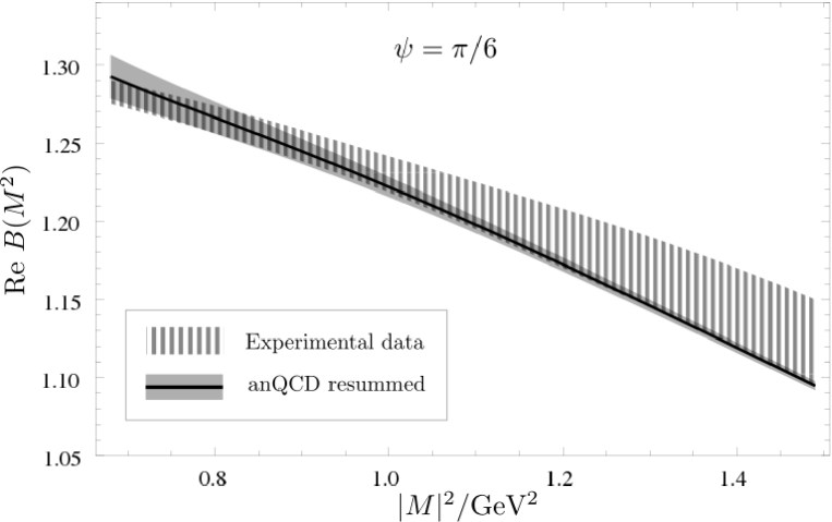
Figure 4: Real part of the Borel transform, Eqs. (72)-(74) and (77), for $M^{2}=|M|^{2}\exp(i\psi)$ with $\psi=\pi/6$. The band with dark vertical stripes represents the experimental data (see footnote 19). The solid line is the best theoretical curve of the resummed expression for $D=0$ Adler function ${\cal D}(Q^{2})$ in 2-delta analytic QCD model (anQCD resummed), obtained by the standard minimization with respect to the central experimental values. It corresponds to the central value of the gluon condensate $\langle aGG\rangle=0.0055\ {\rm GeV}^{4}$. The light grey band represents the variation of this curve when the standard minimization is applied with respect to the values of the upper and lower bounds of the experimental band, and gives the variation of the gluon condensate $0.0055\pm 0.0040\ {\rm GeV}^{4}$.

The results of our analysis for the $\psi=\pi/6$ are given in Fig. 4. Using 2-delta analytic QCD model described in Sec. II and the resummation method of Sec. III for the evaluation of the $D=0$ part, Eq. (75), we obtain for the gluon condensate the values

$$\langle aG^{\alpha}_{\mu\nu}G^{\alpha}_{\mu\nu}\rangle=(0.0055\pm 0.0040_{\rm(exp)}\pm 0.0025_{\rm(oth)})\ {\rm GeV}^{4}=0.0055\pm 0.0047\ {\rm GeV}^{4}\ .$$ (81)

For the parameters of the analytic QCD model we used the central values of the parameters as determined in Ref. 2danQCD , i.e., the second line of Table 1 here. The central condensate value $0.0055\ {\rm GeV}^{4}$ was obtained by adjusting the gluon condensate value in such a way that the theoretical curve (the solid line in Fig. 4) gives the minimal deviation from the central experimental values, in the standard minimization procedure, using $40$ equidistant points over the depicted $|M|^{2}$-interval. The resulting deviation parameter was $\chi^{2}=6.40$. An interesting feature of the resulting best theoretical curve (solid line) is that it remains within the experimental band in almost the entire considered interval of $|M|^{2}$, only slightly surpassing the upper bound of the experimental band at the lowest values of $|M|^{2}$ ($|M|^{2}\approx 0.68\ {\rm GeV}^{2}$).

The uncertainty $\delta\langle aGG\rangle_{\rm exp}=\pm 0.0040\ {\rm GeV}^{4}$ was obtained by applying the same minimization procedure to the upper bounds and lower bounds of the experimental band, respectively. The resulting two theoretical curves then define the upper and the lower border of the light grey band in Fig. 4. This band is thus the prediction of the method (resummed analytic QCD), without the other uncertainties included.

The other uncertainty $\delta\langle aGG\rangle_{\rm oth}=\pm 0.0028\ {\rm GeV}^{4}$ was obtained as the variation of the resummed analytic QCD prediction when the QCD coupling parameter value is varied in its world average interval PDG2010 , $\alpha_{s}^{(\overline{\rm MS})}(M_{Z}^{2})=0.1184\mp 0.0007$; and when the scheme parameter $c_{2}$ of the analytic model is varied according to Table 1, $c_{2}=-4.76_{-0.97}^{+2.66}$. At the end of Sec. II, these two variations in the model are discussed in more detail. The calculations give us for uncertainties of the value of the gluon condensate coming from these two effects: $\delta\langle aGG\rangle_{\rm\alpha_{s}}=_{-0.0025}^{+0.0024}\ {\rm GeV}^{4}$, and $\delta\langle aGG\rangle_{\rm c_{2}}=_{+0.0004}^{+0.0001}\ {\rm GeV}^{4}$. Adding in quadrature then gives us the ”other” uncertainty $\delta\langle aGG\rangle_{\rm oth}\approx\pm 0.0025\ {\rm GeV}^{4}$.

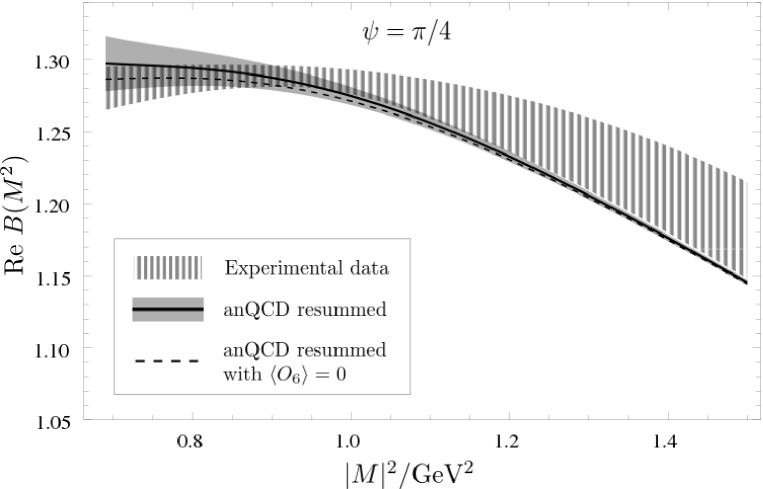
Figure 5: Real part of the Borel transform, Eqs. (72)-(74) and (78), for $M^{2}=|M|^{2}\exp(i\psi)$ with $\psi=\pi/4$. The band with dark vertical stripes represents the experimental data (see footnote 19). The best theoretical curve (solid line) is obtained by standard minimization of the resummed analytic QCD results with respect to the central experimental values. The light grey band is obtained by applying the same minimization to the upper and lower bounds of the experimental band. The dashed curve is the prediction (of the resummed analytic QCD) when $\langle O_{6}^{(V+A)}\rangle=0$. See the text for details.

If we adjust the gluon condensate values, by the same standard minimization method (40 points) with respect to the experimental values, in various evaluation approaches [anQCD resummed; anQCD (truncated); Lambert pQCD resummed; Lambert pQCD (truncated); $\overline{\rm MS}$ (truncated)], we obtain the following values for the gluon condensates, and the corresponding deviation parameter $\chi^{2}$:

$$\langle aGG\rangle = (0.0055\pm 0.0047)\ {\rm GeV}^{4}\ ,\;\chi^{2}=6.40\ ,\quad{\rm(anQCD\ resummed)}\ ,\$$ (82)

$$= (0.0104\pm 0.0058)\ {\rm GeV}^{4}\ ,\;\chi^{2}=9.60\ ,\quad{\rm(anQCD\ truncated)}\ ,\$$

$$= (0.0056\pm 0.0049)\ {\rm GeV}^{4}\ ,\;\chi^{2}=7.42\ ,\quad{\rm(Lambert\ resummed)}\ ,$$

$$= (0.0122\pm 0.0046)\ {\rm GeV}^{4}\ ,\;\chi^{2}=9.83\ ,\quad{\rm(Lambert\ truncated)}\ ,$$

$$= (0.0059\pm 0.0049)\ {\rm GeV}^{4}\ ,\;\chi^{2}=7.43\ ,\quad(\overline{\rm MS}\ {\rm truncated})\ .$$

The uncertainties given above were obtained by adding in quadrature the experimental uncertainty $\delta\langle aGG\rangle_{\rm exp}=\pm 0.0040\ {\rm GeV}^{4}$ and the uncertainty from $\delta\alpha_{s}^{(\overline{\rm MS})}(M_{Z}^{2})=\mp 0.0007$ [$\Rightarrow\ \delta\alpha_{2}^{(\overline{\rm MS})}(m_{\tau}^{2})_{n_{f}=3}=\mp 0.0057$] which is $\delta\langle aGG\rangle_{\rm\alpha_{s}}=\pm 0.0025$, $\pm 0.0025$, $\pm 0.0028$, $\pm 0.0023$, $\pm 0.0028\ {\rm GeV}^{4}$, for the respective five methods above. In the two analytic QCD approaches (anQCD resummed, anQCD truncated) the aforementioned uncertainty coming from $c_{2}=-4.76_{-0.97}^{+2.66}$ is $\delta\langle aGG\rangle_{\rm c_{2}}=_{+0.0004}^{+0.0001}\ {\rm GeV}^{4}$ and ${}_{+0.0012}^{-0.0034}\ {\rm GeV}^{4}$, respectively, and was also added in quadrature. We checked that the gluon condensate values change by less than $2\%$ if the number of points in the standard minimization is decreased from $40$ to $28$; the $\chi^{2}$ values decrease, but the values of ratios of $\chi^{2}$ between different methods are maintained.

It is interesting that the evaluation with the pQCD approach in Lambert scheme (resummed) and in $\overline{\rm MS}$ scheme (not resummed), give similar results for the gluon condensate as in anQCD resummed (and with only somewhat higher $\chi^{2}$).

However, the latter is not the case for the curves when $\psi=\pi/4$ [cf. Eq. (78)]. The results for the case $\psi=\pi/4$ are presented in Fig. 5. The central theoretical curve (solid line) represents the resummed analytic QCD result when the condensate value $\langle O_{6}^{(V+A)}\rangle$ is obtained with the standard minimization (with 40 equidistant points), in complete analogy with the $\psi=\pi/6$ case of Fig. 4. This central value is $\langle O_{6}^{(V+A)}\rangle=-0.5\times 10^{-3}\ {\rm GeV}^{6}$. The resulting deviation parameter is $\chi^{2}=10.79$. The best theoretical curve (solid line) only slightly surpasses the upper bound of the experimental band at low $|M|^{2}<0.7\ {\rm GeV}^{2}$, remains within the experimental band in the interval $0.7\ {\rm GeV}^{2}<|M|^{2}<1.0\ {\rm GeV}^{2}$, and is situated slightly below the lower bound of the experimental band for $1.0\ {\rm GeV}^{2}<|M|^{2}$. It is interesting that the theoretical curve with $\langle O_{6}^{(V+A)}\rangle=0$ (dashed line) is, in comparison, not singificantly worse: it is situated slightly below the lower bound of the experimental band for $0.9\ {\rm GeV}^{2}<|M|^{2}$, and its deviation parameter is $\chi^{2}=12.65$.

The uncertainty $\delta\langle O_{6}^{(V+A)}\rangle_{\rm exp}=\pm 0.9\times 10^{-3}\ {\rm GeV}^{6}$ is obtained by applying the same minimization procedure to the upper bounds and lower bounds of the experimental band, respectively. The resulting two theoretical curves then define the the light grey band in Fig. 5, in analogy with the light grey band of Fig. 4.

The other uncertainty of $D=6$ condensate is estimated as coming from the coupling parameter $\alpha_{s}$ and scheme parameter $c_{2}$ uncertainties, which are: $\delta\langle O_{6}^{(V+A)}\rangle_{\alpha_{s}}=\pm 0.4\times 10^{-3}\ {\rm GeV}^{6}$ and $\delta\langle O_{6}^{(V+A)}\rangle_{c_{2}}=\pm 0.4\times 10^{-3}\ {\rm GeV}^{6}$. Adding in quadrature this gives us $\delta\langle O_{6}^{(V+A)}\rangle_{\rm oth}=\pm 0.6\times 10^{-3}\ {\rm GeV}^{6}$. We thus obtain the following estimate for $D=6$ condensate of the $V$+$A$ channel:

$$\langle O_{6}^{(V+A)}\rangle=(-0.5\pm 0.9_{\rm(exp)}\pm 0.6_{\rm(oth)})\times 10^{-3}\ {\rm GeV}^{6}\approx(-0.5\pm 1.1)\times 10^{-3}\ {\rm GeV}^{6}\ .$$ (83)

The standard minimization gave for the central value a negative number close to zero ($-0.5\times 10^{-3}\ {\rm GeV}^{6}$). The result (83) corresponds approximately to the factorized quark condensate values of Eq. (80)

$$a\langle{\overline{q}}q\rangle^{2}\approx\frac{81}{128\pi^{2}}\langle O_{6}^{(V+A)}\rangle\approx(-3.\pm 7.)\times 10^{-5}\ {\rm GeV}^{6}\ .$$ (84)

We note that the estimates (83)-(84) are not incompatible with nonnegative values. Further, they are not incompatible even with the following positive values of $a\langle{\overline{q}}q\rangle^{2}$ extracted from the $V$-$A$ sum rules of Ref. Ioffe :

$$\langle O_{6}^{(V-A)}\rangle = -(4.4\pm 0.6)\times 10^{-3}\ {\rm GeV}^{6}$$ (85)

$$\Rightarrow\;a\langle{\overline{q}}q\rangle^{2}\left[\approx-\frac{9}{64\pi^{2}\times 1.33}\langle O_{6}^{(V-A)}\rangle\right] \approx (4.7\pm 0.6)\times 10^{-5}\ {\rm GeV}^{6}\ .$$ (86)

It is interesting that the methods other then the resummed analytic QCD approach give us for the central value of $D=6$ condensate significantly more negative values. Specifically, if we adjust in these methods the $D=6$ condensate value by the standard minimization (with 40 equidistant points) to the experimental values, we obtain the following values of the condensate, and of the $\chi^{2}$ fitting parameter:

$$\langle O_{6}^{(V+A)}\rangle = (-0.5\pm 1.1)\times 10^{-3}\ {\rm GeV}^{6}\ ,\;\chi^{2}=10.79\ ,\quad{\rm(anQCD\ resummed)}\ ,\$$ (87)

$$= (-1.9\pm 1.3)\times 10^{-3}\ {\rm GeV}^{6}\ ,\;\chi^{2}=15.75\ ,\quad{\rm(anQCD\ truncated)}\ ,\$$

$$= (-1.8\pm 0.9)\times 10^{-3}\ {\rm GeV}^{6}\ ,\;\chi^{2}=12.23\ ,\quad{\rm(Lambert\ resummed)}\ ,$$

$$= (-2.3\pm 0.9)\times 10^{-3}\ {\rm GeV}^{6}\ ,\;\chi^{2}=16.15\ ,\quad{\rm(Lambert\ truncated)}\ ,$$

$$= (-1.8\pm 0.9)\times 10^{-3}\ {\rm GeV}^{6}\ ,\;\chi^{2}=12.38\ ,\quad(\overline{\rm MS}\ {\rm truncated})\ .$$

The uncertainties above include, in quadrature, the experimental uncertainty $\delta\langle O_{6}\rangle_{\rm exp}=\pm 0.9\times 10^{-3}\ {\rm GeV}^{6}$, and the uncertainty from $\delta\alpha_{s}^{(\overline{\rm MS})}(M_{Z}^{2})=\pm 0.0007$, which is $\delta\langle O_{6}\rangle_{\alpha_{s}}=\pm 0.4\times 10^{-3}\ {\rm GeV}^{6}$ for the two analytic QCD methods, and $\pm 0.3\times 10^{-3}\ {\rm GeV}^{6}$ for the three pQCD methods. In the two analytic QCD approaches (anQCD resummed, anQCD truncated) the uncertainty coming from $c_{2}=-4.76_{-0.97}^{+2.66}$ is $\delta\langle O_{6}\rangle_{\rm c_{2}}=(_{-0.2}^{+0.4})\times 10^{-3}\ {\rm GeV}^{6}$ and $(_{-0.2}^{+0.8})\times 10^{-3}\ {\rm GeV}^{6}$, respectively, and was also included in quadrature. The results of all these methods, with the exception of our central method (anQCD resummed), are incompatible with nonnegative values of $\langle O_{6}^{(V+A)}\rangle$. This agrees also with the analyses of $\tau$-decay data in Refs. O6sr1 ; O6sr2 , where finite energy sum rules were applied (in pQCD+OPE approach) in $\overline{\rm MS}$ scheme. The results (87) thus suggest that the factorization assumption leading to the relation (80) fails to predict correctly even the sign of the condensate, i.e., that it fails much more severely than by $20$-$30\%$ mentioned in Ref. Geshkenbein . On the other hand, the properly resummed analytic QCD (+ OPE) approach gives us the result (83) and (84), suggesting that the relation (80) does not necessarily fail so severely. In fact, the resummed analytic QCD gives for the choice $\langle O_{6}^{(V+A)}\rangle=0$ the value $\chi^{2}=12.65$, which is quite similar to the values $\chi^{2}=12.38,12.23$ obtained by the minimization in $\overline{\rm MS}$ pQCD and Lambert resummed pQCD, respectively (for the central value $\langle O_{6}^{(V+A)}\rangle\approx-1.8\times 10^{-3}\ {\rm GeV}^{6}$).

When we increased the number of (equidistant in $|M|^{2}$) points in the standard minimization procedure from 40 to 60, the values of $\langle O_{6}^{(V+A)}\rangle$ in Eqs. (87) changed very little, and did not affect the digits displayed there; and the corresponding values of $\chi^{2}$ increased proportionally, numerically by about $49$-$50\%$.

Finally, when $\psi=0$, the Borel transform is real and includes, in principle, both condensate contributions ($D=4,6$).

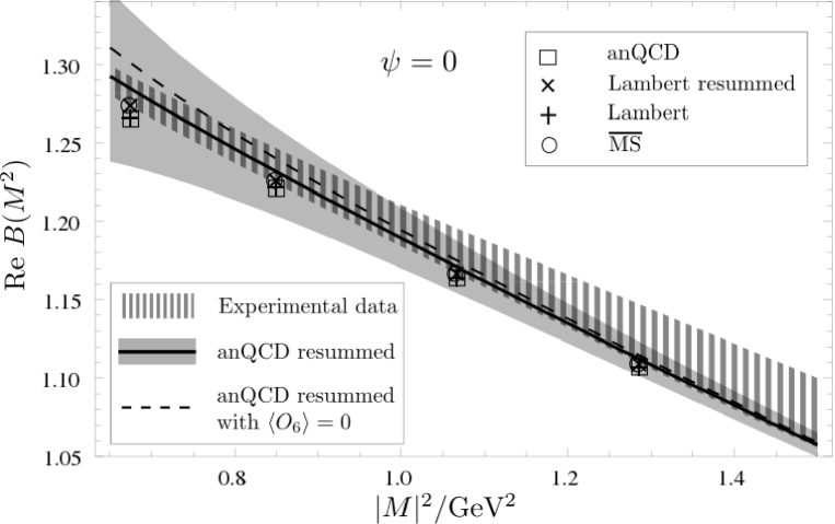
Figure 6: The Borel transform for real $M^{2}=|M|^{2}$ ($\psi=0$). The band with dark vertical stripes represents the experimental data (see footnote 19). The light grey band represents the variation of the resummed 2-delta analytic QCD model prediction (anQCD resummed) when $D=4$ and $D=6$ condensates vary in quadrature around their central values $0.0055\ {\rm GeV}^{4}$ and $-0.5\times 10^{-3}\ {\rm GeV}^{6}$, Eqs. (81) and (83). The central solid curve is for the central values of both condensates. The dashed curve is for the choice $\langle O_{6}^{(V+A)}\rangle=0$ (and $\langle aGG\rangle=0.0055\ {\rm GeV}^{4}$). See the text for details. The results of other methods are given as points, for their corresponding central values of $D=4$ and $D=6$ condensates.

It is presented in Fig. 6. The result of the analytic QCD (with resummed $D=0$ Adler function), for the central values of the condensates, Eqs. (81) and (83), is represented by the central solid curve which is within the experimental band in the entire interval of $M^{2}$. The effects of variation of the values of the two condensates, Eqs. (81) and (83), are also presented in Fig. 6 by the light grey band; the total variations of the two condensates, $\delta\langle O_{2n}\rangle$ ($n=2,3$), are added in quadrature [cf. Eq. (74)]:

$$B(M^{2})_{\rm light\ grey}=B(M^{2};D\!=\!0)+2\pi^{2}\sum_{n=2,3}\frac{\langle O_{2n}\rangle}{(n-1)!\;(M^{2})^{n}}\pm 2\pi^{2}\left[\left(\frac{\delta\langle O_{4}\rangle}{M^{4}}\right)^{2}+\left(\frac{\delta\langle O_{6}\rangle}{2!M^{6}}\right)^{2}\right]^{1/2}\ .$$ (88)

The dashed curve is the result of the choice $\langle O_{6}^{(V+A)}\rangle=0$ (and $\langle aGG\rangle=0.0055\ {\rm GeV}^{4}$). The results of other methods, with their corresponding central values of the condensates, Eqs. (82) and (87), are included as points in Fig. 6. These results are close to the lower bound of the experimental band for all $M^{2}$. The resulting $\chi^{2}$ values (with 40 points), with respect to the central experimental results (with $\psi=0$) are: $\chi^{2}=4.44$ (anQCD resummed); $\chi^{2}=13.44$ (anQCD); $\chi^{2}=7.34$ (Lambert resummed); $\chi^{2}=13.84$ (Lambert); $\chi^{2}=7.58$ ($\overline{\rm MS}$). It is interesting that the dashed line (anQCD resummed with $\langle O_{6}^{(V+A)}\rangle=0$ and $\langle aGG\rangle=0.0055\ {\rm GeV}^{4}$) gives $\chi^{2}=7.02$, which is even slightly less than $\overline{\rm MS}$ (with its own best central values: $\langle O_{6}^{(V+A)}\rangle=-1.8\times 10^{-3}\ {\rm GeV}^{6}$ and $\langle aGG\rangle=0.0059\ {\rm GeV}^{4}$).

V Conclusions

In this work we reanalyzed the Borel sum rules along the rays in the $M^{2}$-complex plane, for the strangeless $V$+$A$ $\tau$-decay invariant-mass spectra of ALEPH Collaboration of 1998. The analysis was performed here with the analytic QCD model developed in Ref. 2danQCD . In this model, the analytic coupling ${\mathcal{A}}_{1}(Q^{2})$ has no unphysical (Landau) singularities, it predicts the correct measured value of $V$+$A$ strangeless decay ratio of $\tau$ lepton, and at high squared momenta it differs from the underlying perturbative coupling $a(Q^{2})$ ($\equiv\alpha_{s}(Q^{2})/\pi$) by terms $\sim(\Lambda^{2}/Q^{2})^{5}$, allowing us to keep the ITEP school interpretation of the OPE expansion up to (and including) dimension-eight ($D=8$) terms. The analysis involves the evaluation of an integral of the $D=0$ Adler function ${\cal D}(Q^{2};D\!=\!0)$ along the contour $|Q^{2}|=m_{\tau}^{2}$. We evaluate this function by applying a generalization of the diagonal Padé resummation, the method being exactly invariant under variation of the renormalization scale and very convenient for application within analytic QCD framework (the latter because no Landau singularities appear). By comparing the experimental ALEPH data of 1998 with the theoretical evaluations for the Borel transform along the argument ray $M^{2}=|M|^{2}\exp(i\psi)$ with $\psi=\pi/6$, we extract with the standard minimization for the ($D=4$) gluon condensate the values $\langle aGG\rangle=(0.0055\pm 0.0047)\ {\rm GeV}^{4}$, cf. Fig. 4 and Eq. (81). Furthermore, considering the ray $\psi=\pi/4$, we analogously extract for $D=6$ condensate the values $\langle O_{6}^{(V+A)}\rangle=(-0.5\pm 1.1)\times 10^{-3}\ {\rm GeV}^{6}$, cf. Fig. 5 and Eqs. (83)-(84). This is not incompatible with the theoretical expectation $\langle O_{6}^{(V+A)}\rangle\propto a\langle{\overline{q}}q\rangle^{2}\geq 0$ based on the factorization (vacuum saturation) approximation. Using the obtained central values of the two condensates, $\langle aGG\rangle=0.0055\ {\rm GeV}^{4}$ and $\langle O_{6}^{(V+A)}\rangle=-0.5\times 10^{-3}\ {\rm GeV}^{6}$, the Borel transform on the real positive axis ($\psi=0$) gives the theoretical curve which remains within the experimental band in the entire analyzed $M^{2}$-interval $(0.68\ {\rm GeV}^{2}<M^{2}<1.5\ {\rm GeV}^{2})$, cf. Fig. 6.

We also compare these results of the resummed analytic QCD approach with those of the not resummed analytic QCD approach and with those of perturbative QCD (pQCD) approaches in two schemes: Lambert scheme of the aformentioned analytic QCD model ($c_{2}\equiv\beta_{2}/\beta_{0}=-4.76$, $c_{3}=c_{2}^{2}/c_{1}$, etc.), and in $\overline{\rm MS}$ scheme ($c_{2}\approx 4.47$, $c_{3}\approx 20.99$). It turns out that in the Lambert scheme pQCD resummed approach and in the $\overline{\rm MS}$ pQCD nonresummed approach the extracted central values of the gluon condensate $\langle aGG\rangle$ are similar, $0.0056$ and $0.0059\ {\rm GeV}^{4}$, respectively, and the $\chi^{2}$ values are only somewhat higher (by about $15\%$). On the other hand, in the not resummed pQCD approach in Lambert scheme, and in the not resummed analytic QCD approach, the extracted values of the gluon condensate are significantly different, with the central value of about $0.0122$ and $0.0104\ {\rm GeV}^{4}$, respectively, and $\chi^{2}$ values are by about $50\%$ higher than in the resummed analytic QCD approach. On the other side, the values of $D=6$ condensate extracted (with $\psi=\pi/4$) in these approaches are negative, $\langle O_{6}^{(V+A)}\rangle\approx(-2\pm 1)\times 10^{-3}\ {\rm GeV}^{6}$, suggesting a complete failure of the vacuum saturation approximation for $\langle O_{6}^{(V+A)}\rangle$ (cf. also Refs. O6sr1 ; O6sr2 on this point). Furthermore, these approaches give us, for their corresponding central values of $D=4$ and $D=6$ condensates, at $\psi=0$ the results which are situated close to the lower edge of the experimental band for all considered $M^{2}$.

Our result for the gluon condensate, $\langle aGG\rangle=(0.0055\pm 0.0047)\ {\rm GeV}^{4}$, is similar to the results of Refs. Geshkenbein ; Ioffe ; O6sr1 . In Ref. Geshkenbein , the value $(0.006\pm 0.012)\ {\rm GeV}^{4}$ was obtained from the $V$+$A$ channel of $\tau$-decay data, and in Ref. Ioffe the value $(0.005\pm 0.004)\ {\rm GeV}^{4}$ from combination of the latter (with ALEPH 1998 data) and of the charmonium sum rules. In Ref. O6sr1 , where ALEPH 2005 data were used, the approach of weighted finite energy sum rules with the contour-improved perturbation theory gave approximately the values $(0.008\pm 0.005)\ {\rm GeV}^{4}$ for the gluon condensate when the standard $\overline{\rm MS}$ QCD scale was ${\overline{\Lambda}}_{n_{f}=3}=0.30$-$0.35$ GeV, the higher values when ${\overline{\Lambda}}=0.3$ GeV and the lower values when ${\overline{\Lambda}}=0.35$ GeV. The original work on the sum rules, Ref. Shifman:1978bx , obtains a higher estimate, of $0.012\ {\rm GeV}^{4}$ from charmonium physics. QCD-moment and QCD-exponential moment sum rules for heavy quarkonia give higher values, $\langle aGG\rangle\approx(0.022\pm 0.004)\ {\rm GeV}^{4}$ and $(0.024\pm 0.006)\ {\rm GeV}^{4}$, respectively, Refs. O4sr1 . On the other hand, in Ref. DDHMZ a combined fit to the $V$+$A$ $\tau$-decay data primarily extracts the value of $\alpha_{s}$ and, as a byproduct, obtains the gluon condensate value $\langle aGG\rangle=(-0.015\pm 0.003)\ {\rm GeV}^{4}$ which differs significantly from the aforementioned values.

The interpretation of our results can be summarized in the following. The nonexistence of the unphysical (Landau) singularities in the running coupling of the (2-delta-parametrized) analytic QCD framework of Ref. 2danQCD leads to a reasonable degree of consistency between the theory and the experiment in the Borel sum rule analysis of the strangeless $V$+$A$ channel of $\tau$-decay physics. To achieve this, it is crucial to perform, in addition, an efficient Padé-related and renormalization scale independent resummation of the Adler function, a method which is very convenient for applications within analytic QCD frameworks precisely because of the absence of the Landau singularities.

Appendix A Renormalization scale independence of parameters in the resummed expression

In this Appendix we show that the dimensionless parameters ${\widetilde{\alpha}}_{j}$ and $\kappa_{j}$ ($j=1,2$), obtained via the construction in Eqs. (48)-(53), are exactly independent of the (dimensionless) renormalization scale parameter $\kappa$ ($\equiv\mu^{2}/Q^{2}$).

We recall that the truncated series ${\widetilde{\cal D}}(Q^{2};\kappa)_{\rm pt}^{[4]}$ of Eq. (48) is made of ${\widetilde{d}}_{n}(\kappa)$ coefficients which are constructed from the coefficients $d_{k}(\kappa)$ of the original power series (25) via the relations (20)-(21), and whose $\kappa$ dependence is a consequence of $\kappa$ independence of the full perturbation series ${\cal D}(Q^{2})_{\rm pt}$ and ${\cal D}(Q^{2})_{\rm mpt}$ of Adler function ${\cal D}(Q^{2})$ (or any spacelike observable) [Eqs. (12)-(13)]. Further, the full series ${\widetilde{\cal D}}(Q^{2})=a_{1\ell}(\kappa Q^{2})+\sum_{n=1}^{\infty}{{\widetilde{d}}}_{n}(\kappa)\;a_{1\ell}(\kappa Q^{2})^{n+1}$ is $\kappa$-independent, because of the differential relations (15).

Let us choose two different renormalization scale parameters, $\kappa$ and $\kappa^{\prime}$, and define the following notations

$$x \equiv a_{1\ell}(\kappa Q^{2})\ ,\qquad x^{\prime}\equiv a_{1\ell}(\kappa^{\prime}Q^{2})\ ,$$ (89)

$$u(\kappa) \equiv \beta_{0}\ln\kappa\ .$$ (90)

The running of the coupling $a_{1\ell}$ is one-loop, Eq. (49). With the notation (90), the quantities ${\widetilde{u}}_{j}(\kappa)$’s appearing in the construction in Eq. (51) [see also Eq. (53)] can be written as

$${\widetilde{u}}_{j}(\kappa)=u(\kappa_{j}/\kappa)\quad\left(=\beta_{0}\ln(\kappa_{j}/\kappa)\right)\ .$$ (91)

It is straightforward to verify from Eq. (49) for the one-loop running coupling that $x$ and $x^{\prime}$ are related by

$$x^{\prime}=\frac{x}{1+u(\kappa^{\prime}/\kappa)x}\ ,$$ (92)

and that the simple fractions appearing in Eq. (51) can be reexpressed as

$$\frac{x}{1+{\widetilde{u}}_{j}(\kappa)x}\;\left(\equiv\frac{x}{1+u(\kappa_{j}/\kappa)x}\right) = \frac{x^{\prime}}{1+u(\kappa_{j}/\kappa^{\prime})x^{\prime}}\ .$$ (93)

Further, it is straightforward to verify that the truncated series ${\widetilde{\cal D}}(Q^{2})_{\rm pt}^{[4]}$ of Eq. (48), while being $\kappa$-dependent due to truncation, at the two renormalization scale parameters $\kappa$ and $\kappa^{\prime}$ differ from each other by $\sim x^{5}$ ($\sim x^{\prime 5}$) terms

$$P_{\kappa^{\prime}}(x^{\prime})-P_{\kappa}(x)\sim x^{\prime 5}\;(\sim x^{5})\ ,$$ (94)

where the two truncated series of Eq. (48) with $\kappa$ and $\kappa^{\prime}$ are denoted as $P_{\kappa}(x)$ and $P_{\kappa^{\prime}}(x^{\prime})$ which are quartic polynomials in $x$ and $x^{\prime}$, respectively

$$P_{\kappa}(x) \equiv {\widetilde{\cal D}}(Q^{2};\kappa)_{\rm pt}^{[4]}=x+\sum_{n=1}^{3}{\widetilde{d}}_{n}(\kappa)x^{n+1}\ ,$$ (95)

$$P_{\kappa^{\prime}}(x^{\prime}) \equiv {\widetilde{\cal D}}(Q^{2};\kappa^{\prime})_{\rm pt}^{[4]}=x^{\prime}+\sum_{n=1}^{3}{\widetilde{d}}_{n}(\kappa^{\prime})x^{\prime n+1}\ .$$ (96)

Namely, the relation (94) follows from the fact that both $P_{\kappa}(x)$ and $P_{\kappa^{\prime}}(x^{\prime})$ differ from the full $\kappa$-independent series ${\widetilde{\cal D}}(Q^{2})=a_{1\ell}(\kappa Q^{2})+\sum_{n=1}^{\infty}{{\widetilde{d}}}_{n}(\kappa)\;a_{1\ell}(\kappa Q^{2})^{n+1}$ by terms $\sim x^{5}$ ($\sim x^{\prime 5}$).

On the other hand, Eq. (93) implies for the sum of simple fractions appearing in the construction of the method, Eq. (51), the following identity:

$$\sum_{j=1}^{2}{\widetilde{\alpha}}_{j}\frac{x}{1+{\widetilde{u}}_{j}(\kappa)x}=\sum_{j=1}^{2}{\widetilde{\alpha}}_{j}\frac{x^{\prime}}{1+u(\kappa_{j}/\kappa^{\prime})x^{\prime}}\ .$$ (97)

The left-hand side of Eq. (97) is, by construction, the diagonal Padé $[2/2]_{P_{\kappa}}(x)$ of the polynomial $P_{\kappa}(x)$ [$\equiv{\widetilde{\cal D}}(Q^{2};\kappa)_{\rm pt}^{[4]}$], cf. Eqs. (50)-(51). Therefore, Eq. (97) in conjunction with Eq. (94) implies that the right-hand side of Eq. (97) is the diagonal Padé $[2/2]_{P_{\kappa^{\prime}}}(x^{\prime})$ of the polynomial $P_{\kappa^{\prime}}(x^{\prime})$ [$\equiv{\widetilde{\cal D}}(Q^{2};\kappa^{\prime})_{\rm pt}^{[4]}$]. More explicitly, we have

$$\sum_{j=1}^{2}{\widetilde{\alpha}}_{j}\frac{x^{\prime}}{1+u(\kappa_{j}/\kappa^{\prime})x^{\prime}}-P_{\kappa^{\prime}}(x^{\prime}) = \left(\sum_{j=1}^{2}{\widetilde{\alpha}}_{j}\frac{x}{1+{\widetilde{u}}_{j}(\kappa)x}-P_{\kappa}(x)\right)+\left(P_{\kappa}(x)-P_{\kappa^{\prime}}(x^{\prime})\right)\sim x^{5}\sim x^{\prime 5}\ .$$ (98)

The difference in the first pair of parentheses on the right-hand side of Eq. (98) is $\sim x^{5}$ because the sum of simple fractions there is, by construction, the diagonal Padé $[2/2]_{P_{\kappa}}(x)$ of the polynomial $P_{\kappa}(x)$; the difference in the second pair of parentheses is $\sim x^{5}$ due to the relation (94). Eq. (98) means that the sum of the simple fractions on the left-hand side there is the diagonal Padé $[2/2]_{P_{\kappa^{\prime}}}(x^{\prime})$ of the polynomial $P_{\kappa^{\prime}}(x^{\prime})$.

However, since $P_{\kappa^{\prime}}(x^{\prime})$ is a polynomial whose coefficients are entirely independent of $\kappa$ (they are only $\kappa^{\prime}$-dependent), this leads to the conclusion that the coefficients of the Padé $[2/2]_{P_{\kappa^{\prime}}}(x^{\prime})$ appearing on the right-hand side of Eq. (97) are $\kappa$-independent, i.e., that ${\widetilde{\alpha}}_{j}$ and $u_{j}(\kappa_{j}/\kappa^{\prime})$ are $\kappa$-independent. This means that $\kappa_{j}$ and ${\widetilde{\alpha}}_{j}$, which were obtained via the construction in Eqs. (48)-(53), are $\kappa$-independent. This concludes the demonstration.

The above argument can be almost literally repeated for the general case of $N=2M$ terms ($M=1,2,3,\ldots$) in the original truncated series (25) and thus in the related truncated series ${\widetilde{\cal D}}(Q^{2};\kappa^{\prime})_{\rm pt}^{[2M]}$. The encountered diagonal Padé’s are now $[M/M]$, and the decomposition in simple fractions is a sum of $M$ simple fractions.

References

- (1) N.N. Bogoliubov and D.V. Shirkov, Introduction to the Theory of Quantum Fields, New York, Wiley, 1959; 1980.
- (2) R. Oehme, Int. J. Mod. Phys. A 10, 1995 (1995) [arXiv:hep-th/9412040].
- (3) D. V. Shirkov and I. L. Solovtsov, hep-ph/9604363; Phys. Rev. Lett. 79, 1209 (1997) [arXiv:hep-ph/9704333].
- (4) K. A. Milton, I. L. Solovtsov and O. P. Solovtsova, Phys. Lett. B 415, 104 (1997) [arXiv:hep-ph/9706409].
- (5) D. V. Shirkov, Theor. Math. Phys. 127, 409 (2001) [hep-ph/0012283]; Eur. Phys. J. C 22, 331 (2001) [hep-ph/0107282].
- (6) K. A. Milton, I. L. Solovtsov, O. P. Solovtsova and V. I. Yasnov, Eur. Phys. J. C 14, 495 (2000) [arXiv:hep-ph/0003030].
- (7) K. A. Milton, I. L. Solovtsov and O. P. Solovtsova, Phys. Rev. D 64, 016005 (2001) [arXiv:hep-ph/0102254].
- (8) M. Baldicchi, A. V. Nesterenko, G. M. Prosperi, D. V. Shirkov and C. Simolo, Phys. Rev. Lett. 99, 242001 (2007); M. Baldicchi, A. V. Nesterenko, G. M. Prosperi, and C. Simolo, Phys. Rev. D 77, 034013 (2008).
- (9) R. S. Pasechnik, D. V. Shirkov and O. V. Teryaev, Phys. Rev. D 78, 071902 (2008) [arXiv:0808.0066 [hep-ph]]; R. S. Pasechnik, D. V. Shirkov, O. V. Teryaev, O. P. Solovtsova and V. L. Khandramai, Phys. Rev. D 81, 016010 (2010) [arXiv:0911.3297]; V. L. Khandramai, R. S. Pasechnik, D. V. Shirkov, O. P. Solovtsova and O. V. Teryaev, Phys. Lett. B 706, 340 (2012) [arXiv:1106.6352 [hep-ph]].
- (10) A. V. Nesterenko and C. Simolo, Comput. Phys. Commun. 181, 1769 (2010) [arXiv:1001.0901 [hep-ph]]; Comput. Phys. Commun. 182, 2303 (2011) [arXiv:1107.1045 [hep-ph]].
- (11) U. Aglietti, G. Ferrera and G. Ricciardi, Nucl. Phys. B 768, 85 (2007) [hep-ph/0608047]; U. Aglietti, F. Di Lodovico, G. Ferrera and G. Ricciardi, Eur. Phys. J. C 59, 831 (2009) [arXiv:0711.0860 [hep-ph]].
- (12) G. M. Prosperi, M. Raciti and C. Simolo, Prog. Part. Nucl. Phys. 58, 387 (2007) [arXiv:hep-ph/0607209].
- (13) D. V. Shirkov and I. L. Solovtsov, Theor. Math. Phys. 150, 132 (2007) [arXiv:hep-ph/0611229].
- (14) A. P. Bakulev, Phys. Part. Nucl. 40, 715 (2009) [arXiv:0805.0829 [hep-ph]] (arXiv preprint in Russian).
- (15) A. V. Nesterenko, Phys. Rev. D 62, 094028 (2000); Phys. Rev. D 64, 116009 (2001); Int. J. Mod. Phys. A 18, 5475 (2003);
- (16) A. V. Nesterenko and J. Papavassiliou, Phys. Rev. D 71, 016009 (2005); A. C. Aguilar, A. V. Nesterenko and J. Papavassiliou, J. Phys. G 31, 997 (2005) [hep-ph/0504195]; Y. .O. Belyakova and A. V. Nesterenko, Int. J. Mod. Phys. A 26, 981 (2011) [arXiv:1011.1148 [hep-ph]].
- (17) R. Barate et al. [ALEPH Collaboration], Eur. Phys. J. C 4, 409 (1998).
- (18) S. Schael et al. [ALEPH Collaboration], Phys. Rept. 421, 191 (2005) [hep-ex/0506072]; M. Davier, A. Höcker and Z. Zhang, Rev. Mod. Phys. 78, 1043 (2006) [hep-ph/0507078].
- (19) M. Davier, S. Descotes-Genon, A. Höcker, B. Malaescu and Z. Zhang, Eur. Phys. J. C 56, 305 (2008) [arXiv:0803.0979 [hep-ph]].
- (20) M. A. Shifman, A. I. Vainshtein and V. I. Zakharov, Nucl. Phys. B 147, 385 (1979); Nucl. Phys. B 147, 448 (1979).
- (21) Y. L. Dokshitzer, G. Marchesini and B. R. Webber, Nucl. Phys. B 469, 93 (1996) [arXiv:hep-ph/9512336].
- (22) G. Cvetič, R. Kögerler, C. Valenzuela, J. Phys. G G37, 075001 (2010) [arXiv:0912.2466 [hep-ph]]; Phys. Rev. D82, 114004 (2010) [arXiv:1006.4199 [hep-ph]].
- (23) C. Contreras, G. Cvetič, O. Espinosa and H. E. Martínez, Phys. Rev. D 82, 074005 (2010) [arXiv:1006.5050].
- (24) C. Ayala, C. Contreras and G. Cvetič, Phys. Rev. D 85, 114043 (2012) [arXiv:1203.6897 [hep-ph]].
- (25) A. I. Alekseev, Few Body Syst. 40, 57 (2006) [arXiv:hep-ph/0503242].
- (26) A. V. Nesterenko, arXiv:1209.0164 [hep-ph].
- (27) S. Peris, M. Perrottet and E. de Rafael, JHEP 9805, 011 (1998) [arXiv:hep-ph/9805442].
- (28) B. A. Magradze, arXiv:1005.2674 [Unknown].
- (29) B. V. Geshkenbein, B. L. Ioffe and K. N. Zyablyuk, Phys. Rev. D 64, 093009 (2001) [arXiv:hep-ph/0104048].
- (30) B. L. Ioffe, Prog. Part. Nucl. Phys. 56, 232 (2006) [arXiv:hep-ph/0502148].
- (31) G. Cvetič and R. Kögerler, Phys. Rev. D 84, 056005 (2011) [arXiv:1107.2902 [hep-ph]].
- (32) B. L. Ioffe and K. N. Zyablyuk, Nucl. Phys. A 687, 437 (2001) [hep-ph/0010089].
- (33) G. Cvetič and C. Valenzuela, J. Phys. G 32, L27 (2006) [arXiv:hep-ph/0601050]; Phys. Rev. D 74, 114030 (2006) [arXiv:hep-ph/0608256].
- (34) G. Cvetič and A. V. Kotikov, J. Phys. G 39, 065005 (2012) [arXiv:1106.4275 [hep-ph]].
- (35) A. P. Bakulev, S. V. Mikhailov and N. G. Stefanis, Phys. Rev. D 72, 074014 (2005) [Erratum-ibid. D 72, 119908 (2005)] [arXiv:hep-ph/0506311]; Phys. Rev. D 75, 056005 (2007) [Erratum-ibid. D 77, 079901 (2008)] [arXiv:hep-ph/0607040]; JHEP 1006, 085 (2010) [arXiv:1004.4125 [hep-ph]]; A. P. Bakulev and I. V. Potapova, Nucl. Phys. Proc. Suppl. 219-220, 193 (2011) [arXiv:1108.6300 [hep-ph]].
- (36) S. Peris, Phys. Rev. D 74, 054013 (2006) [arXiv:hep-ph/0603190].
- (37) G. Cvetič and H. E. Martínez, J. Phys. G 36, 125006 (2009) [arXiv:0907.0033 [hep-ph]].
- (38) G. A. Baker and P. Graves-Morris, Padé Approximants, Encyclopedia of Mathematics and its Applications (Cambridge University, Cambridge, England, 1996).
- (39) MATHEMATICA 8.0.4, Wolfram Co.
- (40) E. Gardi, G. Grunberg and M. Karliner, JHEP 9807, 007 (1998) [hep-ph/9806462].
- (41) D. S. Kourashev, arXiv:hep-ph/9912410.
- (42) D. S. Kurashev and B. A. Magradze, Theor. Math. Phys. 135, 531 (2003) [Teor. Mat. Fiz. 135, 95 (2003)].
- (43) B. A. Magradze, Few Body Syst. 40, 71 (2006) [hep-ph/0512374].
- (44) G. Cvetič and I. Kondrashuk, JHEP 1112, 019 (2011) [arXiv:1110.2545 [hep-ph]].
- (45) K. Nakamura et al. [Particle Data Group], J. Phys. G 37, 075021 (2010).
- (46) K. G. Chetyrkin, B. A. Kniehl and M. Steinhauser, Phys. Rev. Lett. 79, 2184 (1997) [arXiv:hep-ph/9706430].
- (47) D. V. Shirkov, Nucl. Phys. Proc. Suppl. 162, 33 (2006) [arXiv:hep-ph/0611048].
- (48) G. Cvetič, Nucl. Phys. B 517, 506 (1998) [arXiv:hep-ph/9711406]; Phys. Rev. D 57, 3209 (1998) [arXiv:hep-ph/9711487].
- (49) G. Cvetič and R. Kögerler, Nucl. Phys. B 522, 396 (1998) [arXiv:hep-ph/9802248].
- (50) E. Gardi, Phys. Rev. D 56, 68 (1997) [arXiv:hep-ph/9611453].
- (51) K. G. Chetyrkin, A. L. Kataev and F. V. Tkachov, Phys. Lett. B 85, 277 (1979); M. Dine and J. R. Sapirstein, Phys. Rev. Lett. 43, 668 (1979); W. Celmaster and R. J. Gonsalves, Phys. Rev. Lett. 44, 560 (1980).
- (52) S. G. Gorishnii, A. L. Kataev and S. A. Larin, Phys. Lett. B 259, 144 (1991); L. R. Surguladze and M. A. Samuel, Phys. Rev. Lett. 66, 560 (1991) [Erratum-ibid. 66, 2416 (1991)].
- (53) P. A. Baikov, K. G. Chetyrkin and J. H. Kühn, Phys. Rev. Lett. 101, 012002 (2008) [arXiv:0801.1821 [hep-ph]].
- (54) G. Grunberg, Phys. Rev. D 29, 2315 (1984).
- (55) M. Davier, A. Höcker, L. Girlanda, and J. Stern, Phys. Rev. D 58 (1998) 096014 [hep-ph/9802447]; J. Bijnens, E. Gamiz and J. Prades, JHEP 0110, 009 (2001) [hep-ph/0108240]; C. A. Dominguez and K. Schilcher, Phys. Lett. B 581, 193 (2004) [hep-ph/0309285]; S. Friot, D. Greynat and E. de Rafael, JHEP 0410, 043 (2004) [hep-ph/0408281]; S. Narison, Phys. Lett. B 624, 223 (2005) [hep-ph/0412152]; J. Bordes, C. A. Dominguez, J. Penarrocha and K. Schilcher, JHEP 0602, 037 (2006) [hep-ph/0511293]; S. Bodenstein, J. Bordes, C. A. Dominguez, J. Penarrocha and K. Schilcher, Phys. Rev. D 82, 114013 (2010) [arXiv:1009.4325 [hep-ph]]; S. Bodenstein, C. A. Dominguez, S. I. Eidelman, H. Spiesberger and K. Schilcher, JHEP 1201, 039 (2012) [arXiv:1110.2026 [hep-ph]]; and references therein.
- (56) C. A. Dominguez and K. Schilcher, JHEP 0701, 093 (2007) [hep-ph/0611347];
- (57) K. Maltman and T. Yavin, Phys. Rev. D 78, 094020 (2008) [arXiv:0807.0650 [hep-ph]].
- (58) S. Narison, Phys. Lett. B 706, 412 (2012) [arXiv:1105.2922 [hep-ph]]; Phys. Lett. B 707, 259 (2012) [arXiv:1105.5070 [hep-ph]].
- (59) D. Boito, M. Golterman, M. Jamin, A. Mahdavi, K. Maltman, J. Osborne and S. Peris, Phys. Rev. D 85, 093015 (2012) [arXiv:1203.3146 [hep-ph]]; and refences therein.