A sub-determinant approach for pseudo-orbit expansions of spectral determinants in quantum maps and quantum graphs

Abstract

We study implications of unitarity for pseudo-orbit expansions of the spectral determinants of quantum maps and quantum graphs. In particular, we advocate to group pseudo-orbits into sub-determinants. We show explicitly that the cancellation of long orbits is elegantly described on this level and that unitarity can be built in using a simple sub-determinant identity which has a non-trivial interpretation in terms of pseudo-orbits. This identity yields much more detailed relations between pseudo orbits of different length than known previously. We reformulate Newton identities and the spectral density in terms of sub-determinant expansions and point out the implications of the sub-determinant identity for these expressions. We analyse furthermore the effect of the identity on spectral correlation functions such as the auto-correlation and parametric cross correlation functions of the spectral determinant and the spectral form factor.

I Introduction

I.1 Overview

When calculating quantum spectra with the help of periodic-orbit sums such as, for example, arising from semiclassical expressions, one typically encounters problems due to divergencies resulting from summing over a large number of periodic orbits which grows exponentially with length. This is in particular the case for quantum systems whose underlying classical dynamics is chaotic Eck89 . To apply these periodic-orbit expressions for determining quantum spectra, the number of relevant orbits needs to be reduced. This is either achieved by reordering the orbit contributions making use of cancellations such as is done in the cycle expansion Artu or one can also utilise unitarity of the quantum dynamics leading to additional relations between the coefficients of the characteristic polynomial and thus to finite sums over pseudo-orbits Berry ; Tan91 ; Georgeot ; Bog92 ; Bogomolny ; BHJ12 ; Texier .

A related problem is the semiclassical calculation of spectral correlation functions. They are conjectured to follow Random Matrix Theory (RMT) for quantum systems with chaotic classical limit. Establishing this connection explicitly using semiclassical periodic-orbit formulae for the spectral form factor could only be achieved fairly recently following the work in Sieber . This calculation has been extended in Heusler yielding the full spectral form factor as predicted by RMT for times smaller than the Heisenberg time $T_{H}$. (This is the time needed to resolve distances of the order of the mean level spacing in the Fourier-transformed spectrum). The spectral form factor for times larger than $T_{H}$ has been obtained using semiclassical periodic-orbit expressions in HeuslerI . The calculation is based on a generating function approach containing two spectral determinants both in the numerator and denominator at four different energies. The derivation makes explicit use of the fact that the spectral determinant is real for real energies. Although this is obvious from its definition, Eq. (8) below, it is not clear a-priory when considering the representation of the spectral determinant containing periodic-orbit sums. A real spectral determinant in terms of periodic orbits can only be semiclassically obtained by exploiting periodic-orbit correlations due to unitarity.

The above problem illustrates that we need a better understanding of correlations between periodic orbits and in particular correlations between long and short orbits. To analyse these correlations in more detail, we study here quantum unitary dynamics described in terms of finite dimensional unitary matrices, i.e. quantum unitary maps. In this case periodic orbits refer to products of elements of the describing unitary matrix with their indices forming a closed cycle. We give later an interpretation in terms of periodic orbits on quantum graphs Kottos where exact periodic-orbit expansions for spectral quantities exist. These expansions are of similar form as the semiclassical approximations obtained for more general systems. We will in particular advocate to consider spectral quantities in terms of sub-determinant expansions. By this we obtain a much more detailed relation between contributions from orbits of different length for closed systems. The previously known relations Bog92 only connect the overall (summated) contributions to spectral quantities from long and short orbits. We, however, derive a relation between contributions from short orbits within different parts of the system and its corresponding complementary orbits. Such an identity is of particular importance when spatially inhomogeneous effects, such as a magnetic field, that affect the contributions from different orbits of the same length differently are considered. We expect it also to lead to simplifications in the diagrammatic expansions in Texier . We afterwards will derive sub-determinant expressions for a range of important spectral quantities and consider these for examples such as quantum graphs.

The paper is structured as follows: We first introduce the spectral determinant and explain the known implications of unitarity for this quantity. We analyse in Sec. II further implications of unitarity on pseudo-orbit expansions. In this context, we present a sub-determinant identity for unitary matrices and explain how it yields the considered relation between short and long orbit contributions. We discuss the implications of this identity on Newton identities and a pseudo-orbit expansion of the spectral density. In Sec. III, we derive expressions for spectral correlation functions such as the auto-correlation and the parametric cross correlation function of the spectral determinant and the spectral form factor in terms of sub-determinant expansions. Implications due to the sub-determinant identity will be discussed.

I.2 Some basic properties of the characteristic polynomial of a matrix

Consider a general complex matrix $U$ of dimension $N$. Its characteristic polynomial is given by

$$P_{U}(z)\equiv\det\left(z-U\right)=\sum_{n=0}^{N}(-1)^{N-n}a_{N-n}z^{n}=\prod_{n=1}^{N}(z-z_{n}),$$ (1)

where the complex numbers $z_{n}$ are the eigenvalues of $U$. The complex coefficients $a_{n}$ of the polynomial in (1) will be at the centre of interest in this article. Here, $a_{0}=1$ and the remaining $N$ coefficients $a_{n}$, $n=1,\dots,N$, are $N$ complex numbers which contain the same information as the $N$ eigenvalues $z_{n}$. Note that the characteristic polynomial is invariant under conjugation $U\mapsto CUC^{-1}$ with a non-singular matrix $C$. The coefficients $a_{n}$ are thus matrix invariants (as are the eigenvalues) and can be expressed in terms of other matrix invariants such as traces of powers of $U$. Indeed, expressions for the coefficients $a_{n}$ in Eq. (1) in terms of eigenvalues or traces of $U$ can be easily written down, for instance

$$a_{1} = \sum_{n=1}^{N}z_{n}=\mathrm{tr}\,U,$$

$$a_{2} = \frac{1}{2}\sum_{n\neq m}z_{n}z_{m}=\frac{1}{2}\left(\mathrm{tr}^{2}\ U-\mathrm{tr}\ U^{2}\right).$$

Similar formulae expressing the $a_{n}$’s in terms of traces hold for all $n$ fritz_qsc . Note however, that $a_{N}=\prod_{n=1}^{N}z_{n}=\det U$ has a much simpler expression in terms of the determinant of $U$.

Alternatively one may express the coefficients in terms of sub-determinants of $U$. Denote the set $\mathcal{I}=\{1,2,\dots,N\}$ and let $\Gamma\subset\mathcal{I}$ be some subset of $\cal I$ of cardinality $|\Gamma|$. Note that there are $2^{N}-1$ nontrival subsets of $\mathcal{I}$ that we write in the form $\left\{\Gamma\right\}_{j=1}^{2^{N}-1}$. Then $\Gamma$ defines a quadratic $|\Gamma|\times|\Gamma|$ submatrix $U_{\Gamma}$ which is obtained from $U$ by keeping only those rows and columns with indices belonging to $\Gamma$. We will denote the determinant of $U_{\Gamma}$ as

$$d_{\Gamma}=\det U_{\Gamma}\,.$$ (2)

Using the linearity properties of the determinant with respect to its rows (or columns), it is then straight forward to show that

$$a_{n}=\sum_{\Gamma\subset\mathcal{I}:\ |\Gamma|=n}d_{\Gamma}\ .$$ (3)

The sum extends over the ${N\choose n}$ different choices of $n$ rows (and the corresponding columns) that build the sub-matrix $U_{\Gamma}$. While $a_{n}$ is a matrix invariant it is noteworthy that this is in general not the case for the individual contributions $\det U_{\Gamma}$.

II On pseudo-orbit expansions in terms of determinants

II.1 Basic relations

Let us now consider the characteristic polynomial and some related spectral functions for the specific case of unitary matrices $U$. We will keep the discussion general here and will only later refer to $U$ as the evolution matrix for a quantum system.

A unitary matrix $U$ of dimension $N$ has $N$ uni-modular eigenvalues $z_{n}=e^{i\theta_{n}}$. This implies the functional equation

$$P_{U}(z)=(-z)^{N}e^{i\phi}P_{U}(1/z^{*})^{*}$$ (4)

for its characteristic polynomial where $z^{*}$ denotes the complex conjugate of $z$ and $e^{i\phi}=\det\ U=a_{N}$. Comparing coefficients of $z^{n}$ on both sides of the functional equation (4) results in the explicit relation

$$a_{N-n}=e^{i\phi}a_{n}^{*}$$ (5)

between the coefficients of the characteristic polynomial. Below in Sec. II.2, we will generalise this relation to individual determinants of sub-matrices contained in the coefficient $a_{n}$ according to (3).

For unitary maps it is useful to introduce the following variant of the characteristic polynomial, the so called zeta function,

$$\zeta_{U}(\theta)=e^{-iN\theta}P_{U}(e^{i\theta})=\det\left(\mathbbm{I}-e^{-i\theta}U\right)=\sum_{n=0}^{N}(-1)^{n}a_{n}e^{-i\theta n}\ .$$ (6)

This is a $2\pi$ periodic function in the variable $\theta$ which vanishes exactly at the spectrum of real eigenphases $\{\theta_{n}\}_{n=1}^{N}$. In terms of sub-determinants (2) one may also write

$$\zeta_{U}(\theta)=\sum_{\Gamma}d_{\Gamma}e^{-i(\theta+\pi)|\Gamma|}$$ (7)

where the sum is over all subsets $\Gamma\subset\mathcal{I}$ including the empty set $\Gamma=\emptyset$ with $|\Gamma|=|\emptyset|=0$ for which we set $d_{\emptyset}=1$.

The functional equation (4) implies that

$$Z_{U}(\theta)=e^{iN\frac{\theta+\pi}{2}-i\frac{\phi}{2}}\zeta_{U}(\theta),$$ (8)

usually referred to as spectral determinant, is real for real $\theta$, i.e. $Z_{U}(\theta)^{*}=Z_{U}(\theta)$.

Another spectral function which will be discussed later is the density of states

$$\rho(\theta)=\sum_{n=1}^{N}\delta_{2\pi}(\theta-\theta_{n})$$ (9)

where $\delta_{2\pi}(x)\equiv\sum_{n=-\infty}^{\infty}\delta(x+2\pi n)$ is the $2\pi$ periodic $\delta$-comb. The density of states can be expressed as

$$\rho(\theta)=\frac{1}{\pi}\frac{d}{d\theta}\mathrm{Im}\log Z_{U}(\theta-i\epsilon)=\frac{N}{2\pi}+\frac{1}{\pi}\frac{d}{d\theta}\mathrm{Im}\log\zeta_{U}(\theta-i\epsilon)\$$ (10)

in the limit $\epsilon\to 0$. This expression directly leads to the trace formula which expresses the density of states in terms of periodic orbits. We will discuss this in Sec. II.3 together with a novel expansion in terms of sub-determinants presented in the next section.

II.2 A sub-determinant identity for unitary matrices

We here first recapitulate the Jacobi determinant identity applied to the sub-determinants $d_{\Gamma}$ for unitary matrices MathWo which contains much more detailed information than Eq. (5). As this identity is of great relevance in the paper we also give its proof. We will interpret this identity in terms of periodic orbits and will discuss the implications for spectral measures in the remainder of the article.
Theorem: Let $U$ be a unitary matrix of dimension $N$ with determinant $\det U=e^{i\phi}$ and $\Gamma\subset\mathcal{I}\equiv\{1,2,\dots,N\}$ with $n=|\Gamma|$. Denote the complement of $\Gamma$ in $\mathcal{I}$ by $\hat{\Gamma}\equiv\mathcal{I}\setminus\Gamma$. Then the following identity for the determinants of the $n\times n$ submatrix $U_{\Gamma}$ and the $(N-n)\times(N-n)$ submatrix $U_{\hat{\Gamma}}$ holds:

$$\det U_{\Gamma}=e^{i\phi}\left(\det U_{\hat{\Gamma}}\right)^{*}\ .$$ (11)

Proof: Writing $U$, without loss of generality, in block-form

$$U=\left(\begin{array}[]{cc}U_{\Gamma}&V\\ W&U_{\hat{\Gamma}}\end{array}\right)$$ (12)

the identity can be proven by calculating the determinant of both sides of the matrix identity

$$\left(\begin{array}[]{cc}U_{\Gamma}&V\\ W&U_{\hat{\Gamma}}\end{array}\right)\left(\begin{array}[]{cc}\mathbbm{1}&W^{\dagger}\\ 0&U_{\hat{\Gamma}}^{\dagger}\end{array}\right)=\left(\begin{array}[]{cc}U_{\Gamma}&0\\ W&\mathbbm{1}\end{array}\right).$$ (13)

In the last equation the determinant of the first matrix equals $e^{i\phi}$, the second $(\det U_{\hat{\Gamma}})^{*}$ and the third $\det U_{\Gamma}$.                                                                                                                  

This identity implies some fundamental connections between orbits and pseudo-orbits of dynamical systems, which, in our view, are worth exploring. We will discuss these implications in the following sections.

As a straightforward consequence, one obtains for the zeta function (7) for $N$ odd,

$$\zeta_{U}(\theta)=\sum_{\Gamma:|\Gamma|\leq N/2}\left(d_{\Gamma}e^{-i(\theta+\pi)|\Gamma|}+d_{\Gamma}^{*}e^{i\phi}e^{-i(\theta+\pi)(N-|\Gamma|)}\right)\ .$$ (14)

The formula remains true for $N$ even if appropriate care is taken for contributions with $|\Gamma|=N/2$; only half of these contributions should be counted and this half needs to be chosen appropriately. Expression (14) resembles Riemann-Siegel look-alike formulae, see Berry ; Tan91 .

II.3 Pseudo-orbit expansions in terms of determinants

In the previous sections, we have expressed the characteristic polynomial $P_{U}(z)$ and related expressions in terms of the determinants $d_{\Gamma}$. Before we turn to express the density of states or spectral correlation functions in a similar fashion, we will consider how the identity (11) can be interpreted in a periodic orbit language. To this end, we briefly explain what we mean by a ’periodic orbit’ in terms of a finite matrix and introduce some related notation. Analogous finite pseudo-orbit expansions in terms of short orbits have recently been discussed considering relation (5) in the context of quantum graphs BHJ12 . We stress here expansions in terms of sub-determinants which together with Eq. (11) give compact expressions for spectral quantities in terms of short periodic orbits.

II.3.1 Periodic orbit representations

In the present setting of a unitary $N\times N$ matrix a periodic orbit $p=\overline{i_{1}\dots i_{n}}$ of (topological) length $|p|=n$ is a sequence of $n$ integers $i_{m}\in\{1,2,\dots,N\}$ where cyclic permutations are identified, e.g. $\overline{134}=\overline{341}$. One should think of a periodic orbit as a set of indices of the matrix $U$ that are visited in a periodic way. Note that by the term ’periodic orbit’, we do not yet refer to classical orbits in the sense of a continuous classical dynamics, but to products of elements of $U$ with the indices forming a cycle. When considering quantum graphs in Sec. III.3 these ’periodic orbits’ can then indeed be identified with periodic orbits on the graph. A primitive periodic orbit is a sequence $p=\overline{i_{1}\dots i_{n}}$ which is not a repetition of a shorter sequence. If $p$ is not primitive we denote its repetitions number by $r_{p}$. An irreducible periodic orbit never returns to the same index, that is, all $i_{m}$ are different; the length of an irreducible orbit is at most $N$. We also define the (quantum) amplitude

$$t_{p}=\prod_{m=1}^{n}U_{i_{m+1}i_{m}}$$ (15)

of a periodic orbit. If $p$ is not irreducible one may write its amplitude as a product of amplitudes of irreducible orbits, for instance $t_{\overline{1213}}=t_{\overline{12}}t_{\overline{13}}$.

A pseudo-orbit $\gamma=p_{1}^{m_{1}}p_{2}^{m_{2}}\dots p_{n}^{m_{n}}$ with non-negative integers $m_{l}$ is a formal abelian product of periodic orbits $p_{l}$ with length $|\gamma|=\sum_{l}m_{l}|p_{l}|$ and amplitude $t_{\gamma}=\prod_{l}t_{p_{l}}^{m_{l}}$. We will say that a pseudo-orbit is completely reduced if it is a formal product of irreducible orbits and irreducible if all $m_{l}$ are either one or zero and if any given index appears at most in one $p_{l}$ with $m_{l}=1$.

These definitions allow us to write the trace $\mathrm{tr}\ U^{n}=\sum_{p:|p|=n}\frac{n}{r_{p}}t_{p}$ as a sum over amplitudes of periodic orbits of length $n$. Using $\log\det(\mathbbm{1}-e^{-i\theta}U)=\operatorname{tr}\log(\mathbbm{1}-e^{-i\theta}U)$ in (10) and expanding the logarithm one arrives at the trace formula

$$\rho(\theta)=\frac{N}{2\pi}-\frac{1}{\pi}\frac{d}{d\theta}\sum_{p\in\mathcal{P}}\sum_{r=1}^{\infty}\frac{1}{r}t_{p}^{r}e^{-i|p|\theta}$$ (16)

where sum over $p$ extends over the set of all primitive orbits denoted by $\mathcal{P}$, and the additional sum is over all repetitions. Here, like in Eq. (10), it is always understood that $\theta\equiv\theta-i\epsilon$ and the limit $\epsilon\to 0$ is taken.

Performing the sum over repetitions in the trace formula shows that it is equivalent to an Euler-product type expansion

$$\zeta_{U}(\theta)=\prod_{p\in\mathcal{P}}\left(1-t_{p}e^{-i|p|\theta}\right)\ .$$ (17)

Note that this is an infinite product (which converges for $\epsilon>\ln N$) and analytical continuation is necessary to move back to the axis $\epsilon=0$. Such an analytic continuation is of course given by the expression (6) which is by definition a finite polynomial in $z=e^{-i\theta}$. Strong correlations between the amplitudes of long and short periodic orbits have to exist in order to reconcile both expressions. Indeed, large cancellations can be shown to exist by expanding the product (17) and ordering the terms with increasing orbit length such as in the cycle expansion proposed in Artu . After expressing amplitudes of reducible (arbitrarily long) orbits as product of amplitudes of irreducible (and thus short) orbits, the cancellation mechanism emerges Bog92 ; Bogomolny .

Revisiting Eq. (7) and observing that each determinant $d_{\Gamma}$ can indeed be written as a sum of $|\Gamma|!$ irreducible pseudo-orbits $\gamma$ of length $|\gamma|=|\Gamma|$, we obtain

$$d_{\Gamma}=\sum_{\gamma\in P_{\Gamma}}(-1)^{\sigma_{\gamma}+1}t_{\gamma}\,.$$ (18)

Here, $P_{\Gamma}$ is the set of all irreducible pseudo-orbits which cover the set $\Gamma$ completely, that is, which visit each index in $\Gamma$ exactly once. There is a one-to-one correspondence between these irreducible pseudo-orbits and permutations. Indeed any permutation of symbols in $\Gamma$ can be written uniquely as a product of cycles such that each symbol appears exactly once (up to the ordering of the cycles which is irrelevant as they commute). Each such product of cycles, that is, each irreducible pseudo-orbit, defines a unique permutation. We denote the number of cycles (irreducible orbits) that make up a given pseudo-orbit $\gamma$ as $\sigma_{\gamma}$ such that $(-1)^{\sigma_{\gamma}+1}$ gives the parity of the permutation.

II.3.2 Interpretation of the identity (11) in terms of periodic orbits

Everything said in the previous subsection is valid for general, not necessarily unitary matrices. Unitarity leads to further non-trivial relations between the amplitudes of short and long orbits such as the functional equation (4) resulting in the relation (5) for the coefficients of the characteristic polynomial which can in turn be written in terms of orbits.

In Sec. II.2, we showed that there is a much more detailed link between sub-determinants and thus between orbits. The identity (11), $d_{\Gamma}=e^{i\phi}d_{\hat{\Gamma}}^{*}$, also provides a connection between short and long orbits, but it has in addition an interesting interpretation in terms of linking irreducible pseudo-orbits in different parts of ’phase space’. $\Gamma$ and its complement $\hat{\Gamma}$ are by definition disjoint and its union forms the whole set $\mathcal{I}=\{1,2,\dots,N\}$. As stated in Eq. (18), $d_{\Gamma},d_{\hat{\Gamma}}^{*}$ consist of all irreducible orbits and pseudo-orbits which completely cover the set $\Gamma$, $\hat{\Gamma}$, respectively, (passing through every index in each of the sets exactly once). The relation (11) thus implies that the sum over all irreducible pseudo-orbits that cover $\Gamma$ is equivalent in weight to the sum over all irreducible pseudo-orbits that cover its complement $\hat{\Gamma}$. The two contributions from the pseudo-orbits in $\Gamma$ and the complement $\hat{\Gamma}$ yield together a real term in the spectral determinant, as the contributions from $\Gamma$ and $\hat{\Gamma}$ are complex conjugated to each other up to a global phase.

The statements up to now refer to unitary quantum maps with the ’periodic orbits’ obtained from products of elements of $U$ with indices occurring in a periodic manner. Given the close relationship between unitary matrices and quantum maps on the one hand and continuous quantum systems on the other hand, we think that this finding has far reaching consequences. For continuous dynamics, expressions for spectral quantities in terms of classical periodic orbits in phase space exist that are asymptotically valid in the limit $\hbar\rightarrow 0$. The relation (11) suggests that the semiclassical weights associated with periodic orbits and pseudo-orbits of classical maps and flows are spatially correlated at all levels. In particular, summing over all orbits associated with a given subset of the full phase space should yield a total amplitude which is equal to the contribution from the orbits in the complement and both contributions are phase related. In order to make this connection more clear we will consider quantum graphs in Sec. III.3 where the products of matrix elements of $U$ yield directly expansions in terms of periodic orbits on the graph. Here the periodic-orbit expansions are exact, in contrast to the ones for continuous dynamics.

II.3.3 Density of states and Newton identities

We will now consider the density of states and show that it can be expressed in terms of completely reduced pseudo-orbits. Equivalently, one can write it as a sum over products of sub-determinants $d_{\Gamma}$. The latter has the advantage that these expressions keep track of the relation (11) between individual determinants which is lost on the level of pseudo-orbit sums.

Making use of Eq. (10), we would like to express $\log\zeta_{U}$ in terms of sub-determinants. We do this by exploiting the identity

$$-\log(1-x)=\frac{1}{2\pi}\sum_{n=1}^{\infty}(n-1)!\int_{0}^{2\pi}e^{i\alpha n+xe^{-i\alpha}}d\alpha\,,$$ (19)

which formally requires $x<1$. Note for the derivation of Eq. (19) that performing the $\alpha$-integral on the right hand side yields the Taylor expansion of the logarithm. Setting $1-x=\sum_{\Gamma}d_{\Gamma}e^{-i(\theta+\pi)|\Gamma|}$ and using (7), we formally obtain $\log\zeta_{U}$ on the left hand side of Eq. (19). After expanding out the exponentials, interchanging integration and summations and carrying out the integration over $\alpha$, one obtains

$$\log\zeta_{U}(\theta)=-\sum_{\mathbf{m}:|\mathbf{m}|>0}(|{\mathbf{m}}|-1)!e^{-i(\theta+\pi)|\mathbf{m}\Gamma|-i\pi|\mathbf{m}|}\prod_{j}\frac{d_{\Gamma_{j}}^{m_{j}}}{m_{j}!}\ .$$ (20)

Here $\mathbf{m}=(m_{1},\dots,m_{2^{N}-1})$ is a tuple of $2^{N}-1$ non-negative integers and $\Gamma_{1},\dots,\Gamma_{2^{N}-1}$ is some enumeration of all non-empty subsets $\Gamma\subset\mathcal{I}$. The integer $m_{j}$ is the multiplicity of that subset $\Gamma_{j}$ in one contribution to (20). We have also introduced the notations $|\mathbf{m}|=\sum_{j=1}^{2^{N}-1}m_{j}$ and $|\mathbf{m}\Gamma|=\sum_{j=1}^{2^{N}-1}m_{j}|\Gamma_{j}|$. Note that an analogous equation to (20) can be given either in a coarser way in terms of coefficients $a_{n}$ or in a more detailed way in terms of products of irreducible pseudo-orbits. The expression in terms of the determinants $d_{\Gamma}$ is the most detailed one in which the relation (11) between long and short orbits remains explicit.

Before moving on to the density of states let us consider the well known expansion $-\log\zeta_{U}(\theta)=\sum_{n=1}^{\infty}\frac{1}{n}e^{-i\theta n}\operatorname{tr}U^{n}$ and compare the coefficients of $e^{-i\theta n}$ with the corresponding ones in (20). This gives us a direct way to express the $n$-th trace in terms of the sub-determinants $d_{\Gamma}$, that is,

$$\operatorname{tr}U^{n}=n(-1)^{n}\sum_{\mathbf{m}:|\mathbf{m}\Gamma|=n}(|{\mathbf{m}}|-1)!\prod_{j=1}^{2^{N}-1}\frac{(-d_{\Gamma_{j}})^{m_{j}}}{m_{j}!}\ .$$ (21)

This formula is reminiscent of the well-known Newton identities that express the traces of powers of a square matrix in terms of the coefficients of the characteristic polynomial, see for example Ber84 . Indeed, as mentioned above, there is an expression of the form (20) in terms of the coefficients $a_{n}$ instead of the $d_{\Gamma}$. The corresponding derivation of the traces leads to the Newton identities. In (21), we have in fact derived a more detailed identity; it allows us to express the (arbitrarily long) periodic orbits that add up to the traces $\operatorname{tr}U^{n}$ explicitly in terms of pseudo-orbits of length smaller than the matrix size $N$. Furthermore, using (11), one has an explicit expression of traces of any power in terms of pseudo-orbits of maximal length $N/2$. Ordering the sequence $(\Gamma_{1},\dots,\Gamma_{2^{N}-1})$ such that it is non-decreasing in length, then

$$\operatorname{tr}U^{n}=n(-1)^{n}\sum_{\mathbf{m}:|\mathbf{m}\Gamma|=n}(|{\mathbf{m}}|-1)!\prod_{j=1}^{2^{N-1}-1}\frac{(-d_{\Gamma_{j}})^{m_{j}}}{m_{j}!}\prod_{j=2^{N-1}}^{2^{N}-1}\frac{(-d_{\hat{\Gamma}_{j}}^{*}e^{i\phi})^{m_{j}}}{m_{j}!}$$ (22)

gives the $n$-th trace in terms of contributions which can be computed from irreducible orbits of length smaller than $N/2$. In the following it will always be understood that products of the form appearing in (21) may be expressed analogously to (22) in terms of short orbits.

Eventually the density of states follows directly from (20):

$$\rho(\theta)=\frac{N}{2\pi}-\mathrm{Im}\!\!\!\sum_{\mathbf{m}:|\mathbf{m}|>0}\!\!\!\ (|{\mathbf{m}}|-1)!\frac{|{\mathbf{m}}\Gamma|}{\pi}e^{-i(\theta+\pi)|{\mathbf{m}}\Gamma|-i\pi|\mathbf{m}|}\prod_{j}\frac{d_{\Gamma_{j}}^{m_{j}}}{m_{j}!}\ .$$ (23)

III Spectral fluctuations in terms of sub-determinants and short orbits

There is a wide variety of measures for spectral fluctuations which have been considered in the past. We will focus here on expressing spectral measures in terms of sub-determinants and show how the relation (11) can be used to understand the contributions of long orbits. We will in particular consider ensembles of unitary matrices where the ensemble average corresponds to an average over system parameters or disorder. In Sec. III.3 we will also discuss applications which only involve a spectral average for a fixed physical system.

III.1 Spectral fluctuations

For a given ensemble of unitary matrices we denote the ensemble average of some quantity $f(U)$ by $\langle f(U)\rangle_{U}$. In the following, we will consider cross- or auto-correlation functions for the spectral determinant, the density of states and other quantities. We start by giving some general definitions.

III.1.1 The auto-correlation function of the spectral determinant

This auto-correlation function has previously been considered from a RMT-perspective in Refs. Fritz_Marek ; Kettemann and semiclassically in diagonal approximation Kettemann ; gregor_auto ; Muller and beyond Waltner . It is defined in terms of $Z(\theta)$ given in (8) as

$$A = \left\langle\frac{1}{2\pi}\int d\theta\ Z_{U}\left(\theta+\frac{s\pi}{N}\right)Z_{U}\left(\theta-\frac{s\pi}{N}\right)\right\rangle_{U}$$ (24)

$$= e^{is\pi}\sum_{n=0}^{N}\left\langle|a_{n}|^{2}\right\rangle_{U}e^{-i\frac{2\pi sn}{N}}\,.$$

In particular, $A(s)$ is the generating function for the variance $\langle|a_{n}|^{2}\rangle$ of the coefficients of the characteristic polynomial. Note that $|a_{n}|^{2}=|a_{N-n}|^{2}$ ensures that $A(s)$ is a real function. In terms of sub-determinants we find

$$\left\langle|a_{n}|^{2}\right\rangle=\sum_{\Gamma,\Gamma^{\prime}:|\Gamma|=|\Gamma^{\prime}|=n}\left\langle d_{\Gamma}d_{\Gamma^{\prime}}^{*}\right\rangle_{U}\ .$$ (25)

We will show below that this reduces to the diagonal sum $\Gamma=\Gamma^{\prime}$ for some specific ensembles.

III.1.2 Parametric cross correlation for the spectral determinant

Here we use explicitely the more detailed character of the identity (11) compared to the one given in Eq. (5) by considering a spatially inhomogeneous perturbation acting on different contributions to the spectral determinant of the same length in a different manner. Let $U$ be a fixed unitary matrix and define $U_{\tau}:=e^{i\tau P_{v}}U$ where $\tau$ is a real parameter and $P_{v}$ is the projector onto the $v$-th basis state; the corresponding matrix is zero everywhere apart from one unit entry at the $v$-th diagonal position. Physically one may think of the parameter $\tau$ as a variation of a local magnetic field. Denoting the corresponding coefficients of the characteristic polynomial as

$$a_{n}(\tau)=\sum_{\stackrel{{\scriptstyle\Gamma:|\Gamma|=n,}}{{v\notin\Gamma}}}d_{\Gamma}+e^{i\tau}\sum_{\stackrel{{\scriptstyle\Gamma:|\Gamma|=n,}}{{v\in\Gamma}}}d_{\Gamma}\,,$$ (26)

we consider the following parametric correlation function for the spectral determinant:

$$B(\tau) = \left\langle\frac{1}{2\pi}\int d\theta\ Z_{U(\tau)}\left(\theta\right)Z_{U}\left(\theta\right)\right\rangle_{U}$$ (27)

$$= e^{-i\tau/2}\sum_{n=0}^{N}\left\langle a_{n}(\tau)a_{n}(0)^{*}\right\rangle_{U}\ .$$

The above expression reduces the problem to the parametric correlations of the coefficients $a_{n}(\tau)$ which can be expressed as

$$\left\langle a_{n}(\tau)a_{n}(0)^{*}\right\rangle_{U}=\sum_{\Gamma^{\prime}:|\Gamma^{\prime}|=n}\left(\sum_{\stackrel{{\scriptstyle\Gamma:|\Gamma|=n,}}{{v\notin\Gamma}}}\left\langle d_{\Gamma}d_{\Gamma^{\prime}}^{*}\right\rangle+e^{i\tau}\sum_{\stackrel{{\scriptstyle\Gamma:|\Gamma|=n,}}{{v\in\Gamma}}}\left\langle d_{\Gamma}d_{\Gamma^{\prime}}^{*}\right\rangle\right)\ .$$ (28)

The two inner sums are here restricted to sets $\Gamma$ of size $|\Gamma|=n$ such that the marked $v$-th basis state is not in $\Gamma$ for the first inner sum and the marked basis state is an element of $\Gamma$ for the second inner sum. The outer sum over $\Gamma^{\prime}$ is only restricted by $|\Gamma^{\prime}|=n$.

For the quantity $B(\tau)$ we can now reduce the number of terms to $n\leq N/2$ by using the relation $d_{\Gamma}(\tau)=e^{i(\phi+\tau)}d_{\hat{\Gamma}}^{*}(\tau)$, Eq. (11). Note that the relation for the $a_{n}$ in Eq. (5) would not be sufficient here, as the different components contributing to $a_{n}$ are exposed to different magnetic fields.

III.1.3 The spectral two-point correlation function and the form factor

The spectral two-point correlation function is defined as

$$R_{2}(s):=\overline{\Delta}^{2}\left\langle\frac{1}{2\pi}\int_{0}^{2\pi}d\theta\rho(\theta+\overline{\Delta}s/2)\rho(\theta-\overline{\Delta}s/2)\right\rangle_{U}-1$$ (29)

where $\overline{\Delta}=\left(\frac{1}{2\pi}\int_{0}^{2\pi}\rho(\theta)\right)^{-1}=2\pi/N$ is the mean spacing between eigenphases. Expanding the density of states in terms of traces and performing the integral over $\theta$, one obtains the standard expression

$$R_{2}(s)=\frac{2}{N}\sum_{n=1}^{\infty}\cos\left(s\frac{2\pi n}{N}\right)K_{n}\,,$$ (30)

where

$$K_{n}=\frac{1}{N}\left\langle\left|\operatorname{tr}U^{n}\right|^{2}\right\rangle_{U}$$ (31)

is known as the form factor. The form factor played an important role in understanding universal and non-universal aspects of spectral statistics; here we give a new representation in terms of sub-determinants, that is,

$$K_{n}=\frac{n^{2}}{N}\!\!\!\sum_{\mathbf{m},\mathbf{m^{\prime}}:|\mathbf{m}\Gamma|=|\mathbf{m^{\prime}}\Gamma|=n}\!\!\!\left\langle(|{\mathbf{m}}|-1)!(|{\mathbf{m}}^{\prime}|-1)!\prod_{j=1}^{2^{N}-1}\frac{(-d_{\Gamma_{j}})^{m_{j}}(-d_{\Gamma_{j}^{\prime}}^{*})^{m_{j}^{\prime}}}{m_{j}!m_{j}^{\prime}!}\right\rangle_{U}\ \!\!\!.$$

(32)

This is an exact expression for the form factor for any ensemble of unitary matrices. We will show below that for some standard models, the double sum over multiplicities $\mathbf{m}$ and $\mathbf{m^{\prime}}$ can be restricted further.

III.2 Random-matrix theory

Let us now consider unitary $N\times N$ matrices $U$ which are distributed according to the Circular Unitary Ensemble (CUE) – in other words $U$ has a uniform distribution with respect to the Haar-measure on the unitary group $U(N)$. The spectral fluctuations of this ensemble are very well understood with explicit results for a large number of relevant measures. These known results have many implications for the statistical properties of the sub-determinants.

One obtains, for instance, for the correlations of the coefficients $a_{n}$ of the characteristic polynomial Fritz_Marek

$$\langle a_{n}a_{n^{\prime}}^{*}\rangle_{\mathrm{CUE}}=\delta_{nn^{\prime}}\qquad\langle a_{n}a_{n^{\prime}}\rangle_{\mathrm{CUE}}=0\,;$$ (33)

it is straight forward to extend this result to the correlations between sub-determinants. Indeed, any average over CUE is necessarily invariant with respect to conjugation, left multiplication, and right multiplication, that is, $U\mapsto VUV^{\dagger},VU,UV$ with a unitary matrix $V$. As relation (33) has to hold also for every transformed $U$, we can choose $V$ diagonal and get

$$\langle d_{\Gamma}d_{\Gamma^{\prime}}\rangle_{\mathrm{CUE}}=0$$ (34)

and

$$\langle d_{\Gamma}d_{\Gamma^{\prime}}^{*}\rangle_{\mathrm{CUE}}=\delta_{\Gamma\Gamma^{\prime}}c_{\Gamma}\ .$$ (35)

Note that

$$\sum_{\Gamma:|\Gamma|=n}c_{\Gamma}=\langle|a_{n}|^{2}\rangle_{\mathrm{CUE}}=1$$ (36)

where the sum extends over ${N\choose n}$ contributions. Moreover, if $\Gamma$ and $\Gamma^{\prime}$ have the same size, that is, $|\Gamma|=|\Gamma^{\prime}|=n$, invariance of the ensemble average under conjugation with a permutation matrix implies

$$c_{\Gamma}=c_{\Gamma^{\prime}}\equiv c_{n}\qquad c_{n}={N\choose n}^{-1}\ .$$ (37)

Let us now consider the parametric correlation $B(\tau)$ defined in (27). Note that it will not depend on the marked basis state, as the double sum over $\Gamma$ and $\Gamma^{\prime}$ in Eq. (28) only contains diagonal expressions after the CUE-average. Moreover among the ${N\choose n}$ subsets $\Gamma$ of a given size $|\Gamma|=n>0$ there are ${N-1\choose n-1}$ subsets which contain the marked basis state and all give the same contribution such that

$$\left\langle a_{n}(\tau)a_{n}^{*}\right\rangle_{\mathrm{CUE}}=\frac{ne^{i\tau}+N-n}{N}$$ (38)

and

$$B(\tau)_{\mathrm{CUE}}=(N+1)\cos(\tau/2)\ .$$ (39)

Let us finally look at the form factor; the CUE result is

$$K_{n,\mathrm{CUE}}=\begin{cases}{n}/{N}&\text{if $n\leq N$}\\ 1&\text{if $n>N$}.\end{cases}$$ (40)

We may compare this to the CUE average of the form factor expressed in terms of sub-determinants (32). Invariance of the CUE ensemble with respect to group multiplication and unitary conjugation restricts the double sum over multiplicities $\mathbf{m}$ and $\mathbf{m^{\prime}}$ in (32). For example, invariance with respect to multiplication with diagonal unitary matrices implies that only those pairs can survive, for which the corresponding product of sub-determinants $\prod_{j=1}^{2^{N}-1}d_{\Gamma_{j}}^{m_{j}}$ and $\prod_{j=1}^{2^{N}-1}d_{\Gamma_{j}}^{m^{\prime}_{j}}$ visit each basis state with the same multiplicity; here, the multiplicity of a basis state is the number of times a given index appears in any pseudo-orbit of the product $\prod_{j}d_{\Gamma_{j}}^{m_{j}}$. Note that this does not imply $m_{j}=m_{j}^{\prime}$ as there may be many choices for the multiplicities $m_{j}$ of the subsets $\Gamma_{j}$ that result in the same multiplicities of a basis state. Comparing the resulting expression with the exact CUE result (40) one may obtain a large set of identities that have to be obeyed by the correlations among the sub-determinants.

III.3 Quantum graphs

III.3.1 Star graphs - an introduction

A quantum graph is a model for a quantum particle that is confined to a metric graph. To keep the discussion simple we will only discuss star graphs which consist of one central vertex and $N$ peripheral vertices. Each peripheral vertex is connected to the center by a bond (or edge) of finite length $0<L_{b}<\infty$. By $L=\mathrm{diag}(L_{1},\dots,L_{N})$ we denote the diagonal matrix that contains the lengths on its diagonal. On a given bond $b$ we denote by $x_{b}\in(0,L_{b})$ the distance from the central vertex. A scalar wave function on the graph is a collection of $N$ complex (square-integrable) functions $\boldsymbol{\Psi}(x)=(\psi_{1}(x_{1}),\dots,\psi_{N}(x_{N}))$. The wave function is required to solve the free stationary Schrödinger equation on each bond, at given energy $E=k^{2}$. This implies $\psi_{b}(x_{b})=a_{b}\left(e^{ikx_{b}}+e^{-ikx_{b}+2ikL_{b}}\right)$ where $a_{b}$ is the amplitude of the outgoing wave from the central vertex and we have imposed Neumann boundary conditions at the peripheral vertices (at $x_{b}=L_{b}$). The matching conditions at the central vertex are given in terms of a unitary $N\times N$ scattering matrix $S$ which relates the amplitudes $a_{b}$ of outgoing waves to the amplitudes $a_{b}e^{2ikL_{b}}$ of incoming waves by $a_{b}=\sum_{b^{\prime}}S_{bb^{\prime}}e^{2ikL_{b^{\prime}}}a_{b^{\prime}}$. Equivalently

$$\mathbf{a}=U(k)\mathbf{a}$$ (41)

for the quantum map

$$U(k)=T(k)S\qquad\textrm{where}\quad T(k)=e^{2ikL}\ .$$ (42)

This implies that the evolution resulting from $U(k)$ consists of scattering events at the vertices and free evolution on the connecting bonds. This propagation can thus be described by the paths on the graph and the spectral quantities can be expressed in terms of sums over pseudo orbits. In contrast to systems with continuous dynamics, the spectral quantities describing graphs possess exact expressions in terms of periodic orbits. This can be understood by following our derivation of expressions for spectral quantities in terms of $U(k)$. The condition (41) is only satisfied at discrete values of the wave number which form the (wave number) spectrum of the graph. As a side remark let us also note that the above defined quantum map for a star graph also describes the quantum evolution on directed graphs with first-order (Dirac-type) wave operators and bond lengths $2L_{b}$ gregor_auto . A more general quantum graph requires a description in terms of a $2N\times 2N$ matrix Kottos .

Spectra of quantum graphs and spectra of the associated unitary quantum maps $U(k)$ have formed a paradigm of quantum chaos due to the conceptual simplicity of the models. In fact, both types of spectra are to a large extent equivalent berkolaiko and we will focus the present discussion on the spectrum of the quantum map $U(k)$. It can be considered as an ensemble of unitary matrices parametrised by $k$. The corresponding average will be denoted by

$$\left\langle F\left(U(k)\right)\right\rangle_{k}=\lim_{K\to\infty}\frac{1}{K}\int_{0}^{K}dkF\left(U(k)\right)\ .$$ (43)

Note that the wave number $k$ enters the quantum map $U(k)=T(k)S$ only through the diagonal factor $T(k)=e^{2iLk}$.

The sets $\Gamma\subset\mathcal{I}$ in this model are one-to-one related to sub-graphs spanned by the corresponding bonds. The sub-determinants $d_{\Gamma}$ of $U(k)$ can thus be written as

$$d_{\Gamma}=e^{ikL_{\Gamma}}\tilde{d}_{\Gamma}$$ (44)

where $L_{\Gamma}=2\sum_{b\in\Gamma}L_{b}$ is twice the metric length of the sub-graph connected to $\Gamma$ and $\tilde{d}_{\Gamma}=\det S_{\Gamma}$ is the corresponding sub-determinant of the scattering matrix $S$. A generic choice of lengths $L_{b}$ implies that the lengths are rationally independent (incommensurate), which will be assumed in the following. Incommensurability implies that $\left\langle e^{ik\sum_{b=1}^{N}m_{b}L_{b}}\right\rangle_{k}$ does vanish except for $m_{b}=0$ for all $b=1,\dots,N$.

III.3.2 Results for general star graphs

It is straight forward to implement the averages for the spectral fluctuation measures introduced in Sec. III.1. Let us start with the variance of the coefficients of the characteristic polynomial, Eq. (25), which build up the auto-correlation function $A(s)$. Due to the difference in the metric lengths of the corresponding sub-graphs only diagonal entries in the double sum of Eq. (25) survive the average, that is,

$$\left\langle|a_{n}|^{2}\right\rangle_{k}=\sum_{\Gamma:|\Gamma|=n}\left|\tilde{d}_{\Gamma}\right|^{2}\ .$$ (45)

Note that the expression can not reduce further due to averaging. Contributions from different sets $\Gamma$ contain orbits of different length, so non-diagonal contributions made up of products of orbits from different sub-graphs $\Gamma$ do not survive the average; orbits and pseudo-orbits contained in $\tilde{d}_{\Gamma}$ cover the same sub-graph $\Gamma$, and thus have all the same lengths Tanner . In full analogy, we find

$$\left\langle a_{n}(\tau)a_{n}(0)^{*}\right\rangle_{k}=\sum_{\stackrel{{\scriptstyle\Gamma:|\Gamma|=n,}}{{v\notin\Gamma}}}\left|\tilde{d}_{\Gamma}\right|^{2}+e^{i\tau}\sum_{\stackrel{{\scriptstyle\Gamma:|\Gamma|=n,}}{{v\in\Gamma}}}\left|\tilde{d}_{\Gamma}\right|^{2}$$ (46)

for the parametric correlations (28). In contrast to the CUE result this will generally depend on the marked $v$-th basis state.

Furthermore, for the spectral two-point correlations, the form factor reduces to

$$K_{n}=\frac{n^{2}}{N}\sum_{L\in\mathcal{L}_{n}}\sum_{\stackrel{{\scriptstyle\mathbf{m},\mathbf{m^{\prime}}:}}{{L_{\mathbf{m}\Gamma}=L_{\mathbf{m^{\prime}}\Gamma}=L}}}(|{\mathbf{m}}|-1)!(|{\mathbf{m^{\prime}}}|-1)!\prod_{j=1}^{2^{N}-1}\frac{(-\tilde{d}_{\Gamma_{j}})^{m_{j}}(-\tilde{d}_{\Gamma_{j}}^{*})^{m_{j}^{\prime}}}{m_{j}!m_{j}^{\prime}!}$$

(47)

where the $\mathcal{L}_{n}$ is the set of all lengths that are a sum of $n$ (not necessarily different) bond lengths of the graph. We have used the short-hand notation $L_{m\Gamma}=\sum_{j=1}^{N}m_{j}L_{\Gamma_{j}}$. Note that equality of metric length $L_{\mathbf{m}\Gamma}=L_{\mathbf{m^{\prime}}\Gamma}$ implies equality of the topological length $|\mathbf{m}\Gamma|=|\mathbf{m^{\prime}}\Gamma|$ while the opposite is not true. Eq. (47) expresses the form factor as a sum over all possible metric lengths with a fixed number $n$ of bonds and a sum over pairs of completely reduced pseudo-orbits of topological length $n$ of the same metric length.

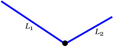
Figure 1: The two-star graph consists of one vertex and two bonds labeled 1 and 2.

III.3.3 The two-star graph

It is instructive to work out the simplest non-trivial case $N=2$ in more detail. In this case the only choices for $\Gamma$ are the empty set, $\Gamma_{1}=\{1\}$, $\Gamma_{2}=\{2\}$ and $\Gamma_{3}=\{1,2\}$ with lengths $L_{\Gamma_{1}}=2L_{1}$, $L_{\Gamma_{2}}=2L_{2}$, and $L_{\Gamma_{3}}=2(L_{1}+L_{2})$, see Fig. 1. The zeta function can be described in terms of the sub-determinant $\tilde{d}_{\Gamma_{1}}=S_{11}$ which is just the reflection amplitude from the first bond and the determinant $\tilde{d}_{\Gamma_{3}}=\det S=e^{i\phi}$ alone; without loss of generality we set $\det S=1$. The remaining relevant sub-determinant is given by $\tilde{d}_{\Gamma_{2}}=S_{22}=\tilde{d}_{\Gamma_{1}}^{*}$ due to (11) and $\det S=1$.

Let us consider how an expansion of the zeta function in terms of periodic orbits and pseudo-orbits as discussed in Sec. II.3 would look like. By expanding the product (17) and reordering the terms according to a cycle expansion Artu , one obtains, for example,

$$\zeta_{U(k)}(\theta) = 1-(t_{1}+t_{2})e^{-i\theta}-(t_{12}-t_{1}t_{2})e^{-2i\theta}$$

$$- (t_{112}-t_{1}t_{12}+t_{122}-t_{12}t_{2})e^{-3i\theta}-\ldots.$$

Writing this out in terms of determinants yields instead

$$\zeta_{U(k)}(\theta) = 1-e^{i2L_{1}k-i\theta}\tilde{d}_{\{1\}}-e^{i2L_{2}k-i\theta}\tilde{d}_{\{1\}}^{*}+e^{i2(L_{1}+L_{2})k-2i\theta}$$

$$= 2e^{i(L_{1}+L_{2})k-i\theta}\left(\cos(2k(L_{1}+L_{2})-\theta)-\Re\left(e^{i(L_{1}-L_{2})k}\tilde{d}_{\{1\}}\right)\right)\,.$$

The cancellation of contributions from longer pseudo-orbits $|p|>2$ appearing in the expansion, Eq. (III.3.3), becomes obvious when writing periodic orbits as completely reduced pseudo-orbits. For example, the contribution $t_{122}$ from the orbit $\{122\}$ is exactly canceled by $t_{12}t_{2}$ from the pseudo-orbit $\{12\}\{2\}$ contributing just with opposite sign. By applying this cancellation mechanism recursively, i.e. reducing the orbits step by step, also the cancellation of contributions from longer pseudo-orbits can be understood. A similar cancellation argument is also used by the cycle expansion. This is however different for the contributions $t_{12}-t_{1}t_{2}$ in (III.3.3). In this case a reduction of the connected orbit leading to cancellation is not possible.

The equivalence between pseudo-orbits on a subset $\Gamma$ and its complements can be made more explicit. The first and the last term in Eq. (III.3.3) resulting from pseudo-orbits of zero length and the length of the full graph, respectively, both have modulus of order 1 and yield a real contribution to $\zeta_{U(k)}(\theta)$ when the phase factor $e^{i\left(L_{1}+L_{2}\right)k-i\theta}$ is taken out. The same holds for the second and the third contributions to Eq. (III.3.3) from the orbits on the set $\Gamma=\{1\}$ and $\Gamma=\{2\}$, respectively. Here, the identity (11) comes in to yield a real contribution (up to an overall pre-factor).

For this simple example, we can calculate the spectral measures discussed in Sec. III.1 explicitly. For the auto-correlation function, Eq. (24), one obtains

$$A(s)=2\cos(\pi s)+2|\tilde{d}_{\Gamma_{1}}|^{2}\ .$$ (50)

For the parametric correlation function, Eq. (27), we consider $U(k;\tau)=\mathrm{diag}(e^{i\tau},1)U(k)$. One then obtains

$$B(\tau)=2\left(1+|\tilde{d}_{\Gamma_{1}}|^{2}\right)\cos(\tau/2)\ .$$ (51)

Eventually, let us consider the form factor $K_{n}$ for a given $n$ as presented in (47). It contains a sum over pairs of multiplicities $\mathbf{m}=(m_{1},m_{2},m_{3})$ and $\mathbf{m^{\prime}}=(m_{1}^{\prime},m_{2}^{\prime},m_{3}^{\prime})$. Both sums are restricted to have the same topological length $|\mathbf{m}\Gamma|=|\mathbf{m^{\prime}}\Gamma|=n$ which implies two restrictions, namely $m_{1}+m_{2}+2m_{3}=n=m_{1}^{\prime}+m_{2}^{\prime}+2m_{3}^{\prime}$. Furthermore only pairs of multiplicities contribute that have the same metric length $L_{\mathbf{m}\Gamma}=L_{\mathbf{m^{\prime}}\Gamma}$ or $L_{1}(m_{1}-m_{1}^{\prime}+m_{3}-m_{3}^{\prime})+L_{2}(m_{2}-m_{2}^{\prime}+m_{3}-m_{3}^{\prime})=0$. The latter implies $m_{1}+m_{3}=m_{1}^{\prime}+m_{3}^{\prime}$ and $m_{2}+m_{3}=m_{2}^{\prime}+m_{3}^{\prime}$. Only three of these four restrictions on pairs of orbits are independent. The form factor can then be written as

$$K_{n} = \frac{n^{2}}{2}\sum_{0\leq m_{3}\leq n/2\atop 0\leq m_{3}^{\prime}\leq n/2}\sum_{0\leq m_{2}\leq n-2m_{3}\atop 0\leq m_{2}^{\prime}\leq n-2m_{3}^{\prime}}\delta_{m_{2}+m_{3},m_{2}^{\prime}+m_{3}^{\prime}}(n-m_{3}-1)!(n-m_{3}^{\prime}-1)!$$ (52)

$$\times\quad{n-2m_{3}\choose m_{2}}{n-2m_{3}^{\prime}\choose m_{2}^{\prime}}\frac{(-1)^{m_{3}+m_{3}^{\prime}}|\tilde{d}_{\Gamma_{1}}|^{2(n-m_{3}-m_{3}^{\prime})}}{m_{3}!m_{3}^{\prime}!(n-2m_{3})!(n-2m_{3}^{\prime})!}\,.$$

Writing the Kronecker as

$$\delta_{m_{2}+m_{3},m_{2}^{\prime}+m_{3}^{\prime}}=\frac{1}{2\pi}\int_{0}^{2\pi}d\alpha\,e^{i\alpha(m_{2}-m_{2}^{\prime}+m_{3}-m_{3}^{\prime})}$$

makes it possible to sum over $m_{2}$ and $m_{2}^{\prime}$ independently. With

$$\sum_{m_{2}=0}^{n-2m_{3}}e^{i\alpha(m_{2}+m_{3})}{n-2m_{3}\choose m_{2}}=(2\cos(\alpha/2))^{n-2m_{3}}e^{i\alpha n/2}$$

and

$$\sum_{m_{2}^{\prime}=0}^{n-2m_{3}^{\prime}}e^{-i\alpha(m_{2}^{\prime}+m_{3}^{\prime})}{n-2m_{3}^{\prime}\choose m_{2}^{\prime}}=(2\cos(\alpha/2))^{n-2m_{3}^{\prime}}e^{-i\alpha n/2},$$

we obtain

$$K_{n} = \frac{n^{2}}{2}\int_{0}^{2\pi}d\alpha\!\!\!\sum_{0\leq m_{3}\leq n/2\atop 0\leq m_{3}^{\prime}\leq n/2}\!\!\!{n-m_{3}\choose m_{3}}{n-m_{3}^{\prime}\choose m_{3}^{\prime}}\frac{(-1)^{m_{3}+m_{3}^{\prime}}|{\tilde{d}}_{\Gamma_{1}}|^{2(n-m_{3}-m_{3}^{\prime})}}{\left(n-m_{3}\right)\left(n-m_{3}^{\prime}\right)}$$ (53)

$$\times\left(2\cos\frac{\alpha}{2}\right)^{2(n-m_{3}-m_{3}^{\prime})}.$$

The sums with respect to $m_{3}$ and $m_{3}^{\prime}$ can be performed by using Prud

$$\sum_{0\leq m_{3}\leq n/2}\frac{(-1)^{m_{3}}}{\left(n-m_{3}\right)}{n-m_{3}\choose m_{3}}x^{2m_{3}} = \frac{1}{2^{n}n}\left[\left(1+\sqrt{1-4x^{2}}\right)^{n}+\right.$$ (54)

$$\left.\left(1-\sqrt{1-4x^{2}}\right)^{n}\right].$$

This yields for $K_{n}$

$$K_{n} = \frac{1}{4\pi}\int_{0}^{2\pi}d\alpha\left[\left(\cos\frac{\alpha}{2}\left|\tilde{d}_{\Gamma_{1}}\right|+\sqrt{\cos^{2}\frac{\alpha}{2}\left|\tilde{d}_{\Gamma_{1}}\right|^{2}-1}\right)^{2n}+\right.$$ (55)

$$\left.\left(\cos\frac{\alpha}{2}\left|\tilde{d}_{\Gamma_{1}}\right|-\sqrt{\cos^{2}\frac{\alpha}{2}\left|\tilde{d}_{\Gamma_{1}}\right|^{2}-1}\right)^{2n}+2\right].$$

The constant term at the end describes the behavior for $n\gg 1$, the other two contributions describe oscillations around the asymptotic value $K_{n}=1$. By taking into account that the arguments of the square roots above are negative, we can rewrite the expression as

$$K_{n}=1+\frac{1}{2\pi}\int_{0}^{2\pi}d\alpha\cos\left[2n\arccos\left(\left|\tilde{d}_{\Gamma_{1}}\right|\cos\frac{\alpha}{2}\right)\right].$$ (56)

The expression in Eq. (56), which we obtained from periodic-orbit expansions, coincides for all $\tilde{d}_{\Gamma_{1}}$ with the result obtained in SchanzI starting from the eigenvalues of the quantum scattering map. This is the first derivation of the result (56) from periodic-orbit expressions for general $\tilde{d}_{\Gamma_{1}}$. In SchanzI , a derivation based on periodic-orbit expressions was only done for $\left|\tilde{d}_{\Gamma_{1}}\right|=1/\sqrt{2}$.

Note that in contrast to Braun_Haake_RS_maps we also take into account contributions beyond the diagonal approximation. Due to the factor $(-1)^{m_{3}+m_{3}^{\prime}}$ appearing in the Eqs. (52, 53) the ones with $m_{3}-m_{3}^{\prime}$ odd contribute with negative signs leading together with the ones with $m_{3}-m_{3}^{\prime}$ even to a form factor smaller than expected in diagonal approximation; as expected it tends to $K=1$ for $n\rightarrow\infty$.

IV Conclusions

The goal of this article is two-fold: first of all, we advocate considering sub-determinant expansions for spectral functions and statistical measures such the density of states or various correlation functions. This makes it possible to separate out contributions which vanish after averaging and those whose non-diagonal contributions survive averaging. Secondly, we considered a sub-determinant identity due to unitarity which makes it possible to give much more detailed relations between short and long orbits on a graph than considered before. In particular, this identity implies that contributions to the characteristic polynomial originating from irreducible pseudo-orbits of a certain sub-graph have the same weight as the irreducible pseudo-orbits of the complement of that sub-graph and are additionally linked through a common phase factor. Previously, only relations between the overall contributions from pseudo orbits of a certain length and the complementary length were studied. The identity leads to simplified expressions for the characteristic polynomial, the Newton identities and the spectral density. Furthermore we study the effect of this identity on spectral correlation functions such as the auto-correlation function of the characteristic polynomial, the parametric cross correlation function and the spectral form factor.

We derive explicit expressions using sub-determinant expansions for a simple model, star graphs consisting of $N$ bonds connected by a single vertex. We then work out in more detail the simplest case $N=2$. The identity (11) is essential to obtaining the behaviour of correlation functions for small energy differences or large times. It captures additional correlations between orbits of different length and needs to be taken into account when singling out correlated orbits which survive averaging. This is especially important when spatial inhomogeneities affect different parts of the phase space in different ways.

In this context several potentially interesting extensions arise: taking the semiclassical limit on both sides of Eq. (22), the two expressions are semiclassically not obviously identical. The left-hand side leads to the Gutzwiller trace formula which contains orbits of arbitrary length while the right-hand side contains pseudo-orbits of finite length (and their repetitions). For short orbits $n\ll N$, one may argue that the two expressions have a semiclassically small difference, for longer orbits this is far less obvious.

A second point concerns the exponential proliferation of the number of orbits in the standard trace formulae. It is tamed to a certain degree when using sub-determinants by the fact that different contributions contribute with different signs. Thus the sub-determinant expressions contain large fluctuations. Understanding overall cancellations is an interesting task. For example, the form factor for the two-star graph for large $n$ contains positive and negative contributions which on their own grow as $n\to\infty$ while their difference remains $\mathcal{O}(1)$ as can be checked from the expressions for $K_{n}$ given above.

The analysis of spectral correlations focused here on the general unitary case. It would be interesting to include the effect of self crossings of orbits that allow for partners traversing parts of the diagram in different directions. This would capture effects arising due to time reversal symmetry.

For graphs the supersymmetry technique gives an alternative approach to obtain universal results SGAA . With supersymmetry one may derive universality under sufficiently nice conditions, however, rigorous proofs are still not available. The main obstacle for the supersymmetric approach seems to be repetitions which are difficult to incorporate correctly GKP . The proposed approach may help us understanding the effect repetitions on spectral correlation functions.

V Acknowledgments

We thank Christopher Eltschka and Jack Kuipers for useful discussions. DW and KR thank the Deutsche Forschungsgemeinschaft (within research unit FOR 760) and DW the Minerva foundation for financial support. SG acknowledges support by the EPSRC research network ’Analysis on Graphs’ (EP/I038217/1).

References

- (1) B. Eckhardt and E. Aurell, Europhys. Lett. 9, 509 (1989).
- (2) R. Artuso, E. Aurell and P. Cvitanovic, Nonlinearity 3, 325 (1990).
- (3) M. V. Berry and J. P. Keating, J. Phys. A 23, 4839 (1990).
- (4) G. Tanner, P. Scherer, E. B. Bogomolny, B. Eckhardt and D. Wintgen, Phys. Rev. Lett. 67, 2410 (1991).
- (5) B. Georgeot and R. E. Prange, Phys. Rev. Lett. 74, 2851 (1995).
- (6) E. B. Bogomolny, Chaos 2, 5 (1992).
- (7) E. B. Bogomolny, Nonlinearity 5, 805 (1992).
- (8) R. Band, J. M. Harrison and C. H. Joyner, J. Phys. A 45, 325204 (2012).
- (9) E. Akkermans, A. Comtet, J. Desbois, G. Montambaux and C. Texier, Ann. Phys. (N.Y.) 284, 10 (2000).
- (10) M. Sieber and K. Richter, Phys. Scr. T 90, 128 (2001).
- (11) S. Müller, S. Heusler, P. Braun, F. Haake and A. Altland, Phys. Rev. Lett. 93, 014103 (2004).
- (12) S. Heusler, S. Müller, A. Altland, P. Braun and F. Haake, Phys. Rev. Lett. 98, 044103 (2007).
- (13) T. Kottos and U. Smilansky, Phys. Rev. Lett. 79, 4794 (1997); Ann. Phys. 274, 76 (1999); S. Gnutzmann and U. Smilansky, Adv. in Phys. 55, 527 (2006).
- (14) F. Haake, Quantum Signatures of Chaos, Springer Series in Synergetics, Springer (2010).
- (15) MathWorld: http://mathworld.wolfram.com/JacobisDeterminantIdentity.html
- (16) E. R. Berlekamp, Algebraic Coding Theory (Aegean Park Press, Laguna Hills, CA) 1984, p. 212.
- (17) F. Haake, M. Kus, H.-J. Sommers, H. Schomerus and K. Zyczkowski, J. Phys. A 29, 3641 (1996).
- (18) S. Kettemann, D. Klakow and U. Smilansky, J. Phys. A 30, 3643 (1997).
- (19) G. Tanner, J. Phys. A 35, 5985 (2002).
- (20) J. P. Keating and S. Müller, Proc. R. Soc. A 463, 3241 (2007)
- (21) D. Waltner, S. Heusler, J. D. Urbina and K. Richter, J. Phys. A 42, 292001 (2009).
- (22) G. Berkolaiko and B. Winn, Trans. Amer. Math. Soc. 362, 6261 (2010).
- (23) G. Tanner, J. Phys. A 33, 3567 (2000).
- (24) A. P. Prudnikov, J. A. Bryckov and O. I. Maricev, Integrals and Series, Vol. 1, Gordon and Breach Science Publ., New York (1986).
- (25) H. Schanz and U. Smilansky, Proc. Australian Summer School on Quantum Chaos and Mesoscopics (1999).
- (26) P. Braun and F. Haake, J. Phys. A 45, 425101 (2012).
- (27) S. Gnutzmann and A. Altland, Phys. Rev. Lett. 93, 194101 (2004); Phys. Rev. E 72, 056215 (2005).
- (28) S. Gnutzmann, J. P. Keating and F. Piotet, Phys. Rev. Lett. 101, 264102 (2008); Annals of Physics 325, 2595 (2010).