2D atom localization in a four-level tripod system in laser fields

Abstract

We propose a scheme for two-dimensional (2D) atom localization in a four-level tripod system under an influence of two orthogonal standing-wave fields. Position information of the atom is retained in the atomic internal states by an additional probe field either of a standing or of a running wave. It is shown that the localization factors depend crucially on the atom-field coupling that results in such spatial structures of populations as spikes, craters and waves. We demonstrate a high-precision localization due to measurement of population in the upper state or in any ground state.

I Introduction

During the last years, spatial localization of an atom using optical techniques has attracted extensive attention. The prototype of an all-optical measuring device is the Heisenberg microscope H . The resolving power of this particular experiment is limited by the optical wavelength if the Heisenberg uncertainty relation is taken into account. Further, in the one-dimensional (1D) case, optical methods for atom localization within the optical wavelength were developed using an internal structure of the atomic levels.

Schemes of subwavelength localization have been performed, using for example, the measurement either of the phase shift Storey ; Storey1 ; Storey2 or of the atomic dipole Kunze after the passage of the atom through an off-resonant standing-wave field. Another method has been proposed by Thomas and co-workers Thomas ; Gardner ; Gardner1 in which a spatially varying potential correlates an atomic resonance frequency with the atomic position. In addition, a few schemes for position measurement were performed, using absorption light masks Zeil ; Zeil1 ; John in which the precision of measurement achieved, was nearly tens of nanometers.

Recently, subwavelength localization of an atom in a standing-wave field was demonstrated in the case of resonant atom-field coupling. For example, two localization schemes were proposed by Zubairy and co-workers using either measurement of the spontaneous spectrum in a three-level system or the resonant fluorescence in a two-level system for localization of the atom during its motion in the standing wave Zub ; Zub1 ; Zub2 ; Zub3 . Another related localization scheme based on measurement of the upper-state population has been proposed by Paspalakis and Knight PK ; PK1 for a three-level $\Lambda$-type atom interacting with two fields, a laser probe field and a classical standing-wave field.

In this paper we demonstrate the two-dimensional (2D) subwavelength localization of an atom in a four-level tripod system due to interaction with a probe laser field and two resonant standing-wave fields. In fact, most 2D level systems consisting of a large number of levels do not match for a subwavelength localization scheme because of interference among states. On the other hand, tripod configuration of atomic levels consists only of four levels involving three atomic ground states and one excited state. We should point out that tripod schemes are experimentally accessible in metastable Ne, ⁸⁷Rb and a number of other gases Th ; Vew .

The paper is organized as follows. In Section II we give the equations of motion of the density-matrix elements in this configuration which are valid for both the running-wave and standing-wave cases of the probe field. In these equations, the spontaneous decay from the upper state to ground states is taken into account. Sections III and IV demonstrate a high-precision localization due to measurement of the upper-state population as well as of a ground-state population. The spatial structures of the populations take the form of spikes, craters or waves depending on the atom-field coupling. Moreover, using measurement of a ground-state population, the atom can be localized at the nodes of the standing waves.

II Model and equations

The laser configuration consists of two parallel $\sigma_{+}$, $\sigma_{-}$ polarized optical waves and an orthogonal linearly polarized optical wave. In such a configuration the positive frequency part of the electric field can be written as

$$\vec{E}^{(+)}(\vec{r},t)=\vec{E}_{1}(x)e^{-i\omega_{1}t}+\vec{E}_{3}(x)e^{-i\omega_{3}t}+\vec{E}_{2}(y)e^{-i\omega_{2}t}.$$ (1)

The first term corresponds to a $\sigma_{+}$ circularly polarized wave with the frequency $\omega_{1}$ and the second one corresponds to a $\sigma_{-}$ circularly polarized wave with the frequency $\omega_{3}$. The third term describes a linearly polarized wave with the frequency $\omega_{2}$. The electrical fields of the standing waves are $\vec{E}_{1}(x)=\vec{\mathcal{E}}_{1}\sin kx$ and $\vec{E}_{2}(y)=\vec{\mathcal{E}}_{2}\sin ky$, while the $\vec{E}_{3}(x)$ corresponds to an additional probe field. The probe field can be either a running wave $\vec{E}_{3}(x)=\vec{\mathcal{E}}_{3}\exp(ikx)$ along the $x$ direction or a standing wave $\vec{E}_{3}(x)=\vec{\mathcal{E}}_{3}\sin(kx+\psi)$ where $\psi$ is the spatial phase shift between the standing waves $\vec{E}_{1}(x)$ and $\vec{E}_{3}(x)$.

(a)
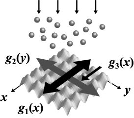
(b)

Figure 1: (a) Atoms pass through an interaction range of coupling with two standing-wave laser fields with the Rabi frequencies $g_{1}(x)$, $g_{2}(y)$ and probe laser field with the Rabi frequency $g_{3}(x)$. (b) A tripod scheme of atomic energy levels. Standing-wave field $g_{1}(x)$ is nearly resonant with the $|1\rangle\leftrightarrow|4\rangle$ transition and the second standing-wave field—$g_{2}(x)$ is nearly resonant with the $|2\rangle\leftrightarrow|4\rangle$ transition, while the probe laser field interacts with the $|3\rangle\leftrightarrow|4\rangle$ transition.

The atom moves parallel to the $z$ axis and passes through the interaction range as seen in Fig. 1(a). The tripod scheme of the atomic levels which has the upper state $|4\rangle$ and the three ground states $|1\rangle$–$|3\rangle$ is shown in Fig. 1(b). The transition $|1\rangle\leftrightarrow|4\rangle$ is taken to be nearly resonant with the standing wave $\vec{E}_{1}(x)$ with the detuning $\Delta_{1}=\omega_{1}-\omega_{41}$, while the transition $|2\rangle\leftrightarrow|4\rangle$ is taken to be nearly resonant with the standing wave $\vec{E}_{2}(y)$ with the detuning $\Delta_{2}=\omega_{2}-\omega_{42}$. The atom interacts with the probe laser field $\vec{E}_{3}(x)$, which is resonant with the $|3\rangle\leftrightarrow|4\rangle$ transition, with the detuning $\Delta_{3}=\omega_{3}-\omega_{43}$.

The coupling of the atom with each of the strong standing waves is characterized by the Rabi frequencies

$$g_{1}(x)=G_{1}\sin kx,\quad g_{2}(y)=G_{2}\sin ky,$$ (2)

where $G_{j}=|\vec{d}_{4j}\vec{\mathcal{E}}_{j}/\hbar|$ ($j=1,2$). The Rabi frequency of the probe field is

$$g_{3}(x)=\left\{\begin{array}[]{cl}\Omega&\mbox{in a running-wave case},\\ \Omega\sin(kx+\psi)&\mbox{in a standing-wave case},\end{array}\right.$$ (5)

where $\Omega=|\vec{d}_{43}\vec{\mathcal{E}}_{3}/\hbar|$.

We assume that the center-of-mass position of the atom is nearly constant along the directions of the laser waves and neglect the kinetic part of the atom from the Hamiltonian in the Raman-Nath approximation Meystre . Note that during the interaction the atomic position does not change directly and our localization scheme only influences the internal states of the atom. Then, in the interaction picture and the rotating wave approximation the equations of matrix-density elements can be written as

$$i\dot{\rho}_{11}=g_{1}(x)(\rho_{14}-\rho_{41})+i\gamma_{1}\rho_{44},$$ (6a)

$$i\dot{\rho}_{22}=g_{2}(y)(\rho_{24}-\rho_{42})+i\gamma_{2}\rho_{44},$$ (6b)

$$i\dot{\rho}_{33}=g_{3}(x)(\rho_{34}-\rho_{43})+i\gamma_{3}\rho_{44},$$ (6c)

$$i\dot{\rho}_{44}=g_{1}(x)(\rho_{41}-\rho_{14})+g_{2}(y)(\rho_{42}-\rho_{24})$$

$$+g_{3}(x)(\rho_{43}-\rho_{34})-2i\gamma\rho_{44},$$ (6d)

$$i\dot{\rho}_{12}=g_{2}(y)\rho_{14}-g_{1}(x)\rho_{42}+(\Delta_{12}-i\Gamma_{12})\rho_{12},$$ (6e)

$$i\dot{\rho}_{13}=g_{3}(x)\rho_{14}-g_{1}(x)\rho_{43}+(\Delta_{13}-i\Gamma_{13})\rho_{13},$$ (6f)

$$i\dot{\rho}_{23}=g_{3}(x)\rho_{24}-g_{2}(y)\rho_{43}+(\Delta_{23}-i\Gamma_{23})\rho_{23},$$ (6g)

$$i\dot{\rho}_{14}=g_{1}(x)(\rho_{11}-\rho_{44})+g_{2}(y)\rho_{12}$$

$$+g_{3}(x)\rho_{13}+(\Delta_{1}-i\Gamma_{14})\rho_{14},$$ (6h)

$$i\dot{\rho}_{24}=g_{2}(y)(\rho_{22}-\rho_{44})+g_{1}(x)\rho_{21}$$

$$+g_{3}(x)\rho_{23}+(\Delta_{2}-i\Gamma_{24})\rho_{24},$$ (6i)

$$i\dot{\rho}_{34}=g_{3}(x)(\rho_{33}-\rho_{44})+g_{1}(x)\rho_{31}$$

$$+g_{2}(y)\rho_{32}+(\Delta_{3}-i\Gamma_{34})\rho_{34},$$ (6j)

together with $\rho_{mn}=\rho_{nm}^{*}$, $\sum\limits_{n=1}^{4}\rho_{nn}=1$ and $\Delta_{mn}=\Delta_{m}-\Delta_{n}$. The atomic decay takes place from the level $|4\rangle$ to the levels $|1\rangle,|2\rangle,|3\rangle$ with the rates $\gamma_{1}$, $\gamma_{2}$ and $\gamma_{3}$, respectively. The decay rates of atomic coherences between the upper level and ground levels equal $\Gamma_{14}$, $\Gamma_{24}$ and $\Gamma_{34}$. Coherent decay rates $\Gamma_{12}$, $\Gamma_{13}$ and $\Gamma_{23}$ are usually much less than the rates of decay through the $|4\rangle\leftrightarrow|m\rangle$ ($m=1,2,3$) channels, so the approximate equalities are $\Gamma_{12}=\Gamma_{13}=\Gamma_{23}=0$.

III 2D atom localization via the upper-level population

The dynamics of interaction vary depending on the position of the atom which passes through laser fields in the $(x,y)$ position. In case of a long-time interaction the final populations in internal states are defined only by the laser fields and the atom does not need an initial-state preparation. The final distribution of the upper-level population depends on three controllable detunings $\Delta_{1}$, $\Delta_{2}$ and $\Delta_{3}$, and on the Rabi frequencies of the driving fields, $G_{1}$, $G_{2}$ and $\Omega$. Also, in a standing-wave case of the probe field the distribution depends on spatial shift $\psi$. Consequently, controlling the parameters of this interaction allows us to create different patterns of the upper-level population.

When the probe laser field is weak the measurement of the upper-state population leads to a high-precision localization, as shown in the related 1D scheme for a three-level $\Lambda$-type atom PK ; PK1 . We assume that $\Omega\ll G_{1},G_{2},\gamma_{m},\Gamma_{m4},|\Delta_{m}|,|\Delta_{mn}|$ ($m,n=1,2,3)$ is satisfied and obtain the long-time population in state $|4\rangle$ in second order of perturbation theory. Note that the second-order perturbation theory is correct only when $\Omega\ll g_{1}(x),g_{2}(y)$, which corresponds to the atomic positions far from the nodes of standing waves $g_{1}(x)$ and $g_{2}(y)$.

In the limit case of $\Omega=0$ the atomic population is concentrated in the $|3\rangle$ state. Therefore, when the probe laser field is weak, we have $\rho_{33}\approx 1$ during the atom-field interaction. In long-time limit, $\dot{\rho}_{mn}=0$ and the non-diagonal elements $\rho_{31}$ and $\rho_{32}$ can be derived from (6f) and (6g) equations and are given by

$$\rho_{31}\approx\frac{g_{1}(x)}{\Delta_{13}}\rho_{34},\quad\rho_{32}\approx\frac{g_{2}(y)}{\Delta_{23}}\rho_{34}.$$ (7)

Here we used a correlation $\rho^{*}_{ij}=\rho_{ji}$. Substitution of Eq. (7) and an approximate expression $\rho_{33}-\rho_{44}\approx 1$ into (6j) gives the non-diagonal element

$$\rho_{34}\approx\frac{g_{3}(x)}{i\Gamma_{34}-\dfrac{g_{1}^{2}(x)}{\Delta_{13}}-\dfrac{g_{2}^{2}(y)}{\Delta_{23}}-\Delta_{3}}.$$ (8)

Then, the upper-level population is obtained from Eq. (6c) and is given by

$$\rho_{44}\approx-\frac{2g_{3}^{2}(x)}{\gamma_{3}}\mathop{\rm Im}\frac{1}{i\Gamma_{34}-\dfrac{g_{1}^{2}(x)}{\Delta_{13}}-\dfrac{g_{2}^{2}(y)}{\Delta_{23}}-\Delta_{3}}.$$ (9)

This expression can be written as

$$\rho_{44}\approx\frac{2\Gamma_{34}g_{3}^{2}(x)}{\gamma_{3}Z},$$ (10)

where

$$Z=\left(\frac{G_{1}^{2}}{\Delta_{13}}\sin^{2}kx+\frac{G_{2}^{2}}{\Delta_{23}}\sin^{2}ky+\Delta_{3}\right)^{2}+\Gamma_{34}^{2}.$$ (11)

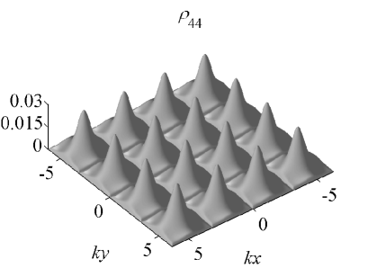
(a)

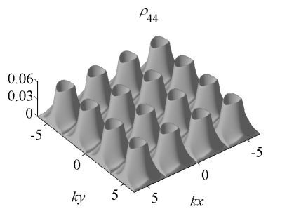
(b)

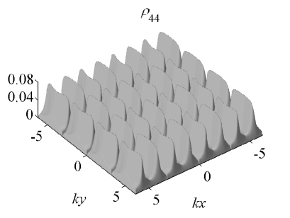
(c)

Figure 2: The upper-level population $\rho_{44}$ as a function of $(kx,ky)$. The spatial distributions of the population represent such 2D periodic structures as (a) spikes, (b) craters and (c) waves in dependence on the laser frequency detunings, (a) $\Delta_{1}=10\gamma$, $\Delta_{2}=14\gamma$, $\Delta_{3}=16\gamma$; (b) $\Delta_{1}=5\gamma$, $\Delta_{2}=9\gamma$, $\Delta_{3}=11\gamma$; and (c) $\Delta_{1}=\gamma$, $\Delta_{2}=-3\gamma$, $\Delta_{3}=5\gamma$. The Rabi frequencies of the standing waves are $G_{1}=6\gamma$, $G_{2}=4\gamma$, and the Rabi frequency of the probe running wave is $\Omega=0.3\gamma$. Other parameters are as follows. Decay rates $\gamma_{1,2,3}$ from the upper level equal $\gamma$, coherent-decay rates through the channels $|4\rangle\leftrightarrow|m\rangle$ ($m=1,2,3$) are $\gamma_{14}=1.5\gamma$, $\gamma_{24}=1.5\gamma$, $\gamma_{24}=1.5\gamma$, and coherent-decay rates among ground states are $\gamma_{12}=0$, $\gamma_{13}=0$, $\gamma_{23}=0$.

The expressions (10), (11) allows us to analyze distribution of the upper-level population. However, the upper-level population given by (10) is correct far from the nodes of standing waves $g_{1}(x)$ and $g_{2}(y)$, where the atomic population is almost entirely in the $|3\rangle$ state. On the other hand, at the nodes of the standing waves expression $g_{1}(x)=0$ or $g_{2}(y)=0$ is satisfied. Hence, the atomic population at the nodes is concentrated either in the $|1\rangle$ state or in the $|2\rangle$ state and the upper-level population at the nodes is zero.

Let us consider a running-wave case of the probe field, when $g_{3}(x)=\Omega$. From (10), (11) we selected three types of distribution of the upper-level population and called them spikes, craters and waves. These types can be seen in Fig. 2 where the upper-level population is obtained by numerically solving Eqs. (6) in the long-time limit.

One can see from (11) that the peaks of the spikes occur in the $(x,y)$ positions given by

$$\sin^{2}kx\approx 1,\quad\sin^{2}ky\approx 1.$$ (12)

These positions are

$$(x,y)\approx(\>(2m+1)\lambda/4,\>(2n+1)\lambda/4\>)$$ (13)

with $\lambda=2\pi/k$ and $m$, $n$ are integer. Thus, the spikes give information how close the atom passes by the points (13) and in case of narrow spikes lead to localization of the atom at these points. The craters in their turn allow one to localize the atom at a distance from the positions (13). The positions of peaks of the craters follow from (11) and are derived from expression

$$\frac{G_{1}^{2}}{\Delta_{13}}\sin^{2}kx+\frac{G_{2}^{2}}{\Delta_{23}}\sin^{2}ky+\Delta_{3}\approx 0.$$ (14)

In case of waves the positions of peaks are given by (14) as well. In this case, by adjusting parameters of the atom-field coupling, we can arrive at the condition

$$\left|G_{2}^{2}/\Delta_{23}\right|\ll\left|G_{1}^{2}/\Delta_{13}\right|.$$ (15)

From (14) we then obtain that the expression

$$\sin^{2}kx\approx\Delta_{3}(\Delta_{3}-\Delta_{1})/G_{1}^{2}$$ (16)

is valid and the atom can be localized along the $x$ direction at the positions (16). Also in case of waves we can realize the following condition

$$\left|G_{1}^{2}/\Delta_{13}\right|\ll\left|G_{2}^{2}/\Delta_{23}\right|,$$ (17)

which leads to localization of the atom at the $y$ positions given by

$$\sin^{2}ky\approx\Delta_{3}(\Delta_{3}-\Delta_{2})/G_{2}^{2}.$$ (18)

The degree of localization in case of spikes, craters or waves is not limited by the optical wavelength and the width of peaks can be essentially smaller than optical wavelength. A high-precision localization is attained by increasing the Rabi frequencies $G_{1}$ and $G_{2}$, while the height of the peaks is defined by the intensity $\Omega^{2}$ of the probe field.

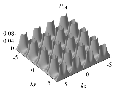
(a)

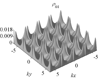
(b)

Figure 3: Transferring the upper-level population by a spatial phase shift of $\pi/2$ along the $x$ or $y$ direction: (a) craters shifted along the $y$ direction to the nodes of standing wave $g_{2}(y)$; (b) spikes shifted to crossings of the nodal lines. The laser frequency detunings are (a) $\Delta_{1}=-3\gamma$, $\Delta_{2}=5\gamma$, $\Delta_{3}=3\gamma$, and (b) $\Delta_{1}=8\gamma$, $\Delta_{2}=4\gamma$, $\Delta_{3}=2\gamma$. The Rabi frequencies of the standing waves are $G_{1}=6\gamma$, $G_{2}=4\gamma$, and the Rabi frequency of the probe running wave is $\Omega=0.3\gamma$. All other parameters are the same as in Fig. 2.

Let us show that the distribution of the upper-state population can be transferred by a spatial phase shift of $\pi/2$ in the $x$ or $y$ direction. In a running-wave case of the probe field spatial dependence of the upper-level population is defined by the denominator (11). The following transformations

$$\Delta^{\prime}_{1}= 2\Delta_{3}-\Delta_{1}+G_{1}^{2}/\Delta_{13},$$ (19)

$$\Delta^{\prime}_{2}= \Delta_{2}+G_{1}^{2}/\Delta_{13},$$

$$\Delta^{\prime}_{3}= \Delta_{3}+G_{1}^{2}/\Delta_{13}$$

convert this denominator to the form

$$Z^{\prime}=\left(\frac{G_{1}^{2}}{\Delta^{\prime}_{13}}\sin^{2}kx+\frac{G_{2}^{2}}{\Delta^{\prime}_{23}}\sin^{2}ky+\Delta^{\prime}_{3}\right)^{2}+\Gamma_{34}^{2}$$

$$=\left(\frac{G_{1}^{2}}{\Delta_{13}}\sin^{2}\left(kx\pm\frac{\pi}{2}\right)+\frac{G_{2}^{2}}{\Delta_{23}}\sin^{2}ky+\Delta_{3}\right)^{2}+\Gamma_{34}^{2},$$ (20)

while the transformations

$$\Delta^{\prime\prime}_{1}= \Delta_{1}+G_{2}^{2}/\Delta_{23},$$ (21)

$$\Delta^{\prime\prime}_{2}= 2\Delta_{3}-\Delta_{2}+G_{2}^{2}/\Delta_{23},$$

$$\Delta^{\prime\prime}_{3}= \Delta_{3}+G_{2}^{2}/\Delta_{23}$$

change the denominator to the next form:

$$Z^{\prime\prime}=\left(\frac{G_{1}^{2}}{\Delta_{13}}\sin^{2}kx+\frac{G_{2}^{2}}{\Delta_{23}}\sin^{2}\left(ky\pm\frac{\pi}{2}\right)+\Delta_{3}\right)^{2}+\Gamma_{34}^{2}.$$ (22)

One can see that the expressions (20), (22) describe the upper-level population (10) shifted by a spatial phase shift of $\pi/2$ along either the $x$ or $y$ axis.

Figure 3 depicts the upper-level population obtained numerically from Eqs. (6) that illustrates the result of employing the transformations (20), (22). Figure 3(a) shows craters after shifting along the $y$ direction to the nodes of standing wave $g_{2}(y)$ and Fig. 3(b) shows spikes after shifting to crossings of the nodal lines. These structures are located near the nodes of the standing waves and take a new form due to crossing by the nodal lines.

In a standing-wave case of the probe field, when $g_{3}(x)=\Omega\sin(kx+\psi)$, the upper-state population essentially decreases near the nodes of the probe field. On the other hand, by adjusting the spatial phase shift $\psi$, most of the upper-level population can be concentrated far from the nodes of the probe field. Then, distribution of the population takes the form similar to the running-wave case of the probe field and the spatial structures look like those in Figs. 2, 3.

IV 2D atom localization via a ground-level population

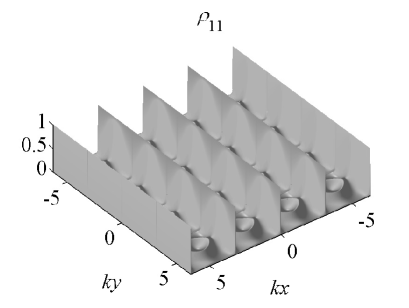
(a)

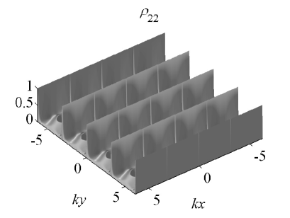
(b)

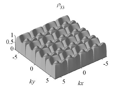
(c)

Figure 4: The ground-state populations as functions of $(kx,ky)$. (a) Population in state $|1\rangle$ has narrow peaks along the nodal lines of standing wave $g_{1}(x)$; (b) population in state $|2\rangle$ has narrow peaks along the nodal lines of standing wave $g_{2}(y)$; (c) population in state $|3\rangle$ has narrow peaks along the nodal lines of both standing waves. The laser frequency detunings are $\Delta_{1}=5\gamma$, $\Delta_{2}=9\gamma$, $\Delta_{3}=11\gamma$; the Rabi frequencies of the standing waves are $G_{1}=6\gamma$, $G_{2}=4\gamma$, and the Rabi frequency of the probe running wave is $\Omega=0.3\gamma$. All other parameters are the same as in Fig. 2.

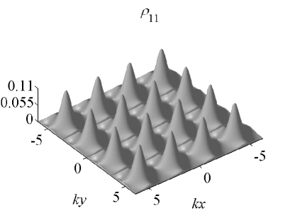
(a)

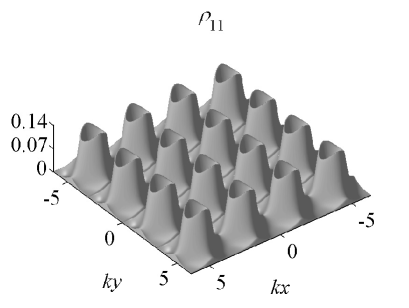
(b)

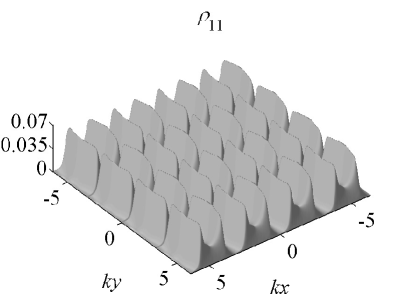
(c)

Figure 5: The population in ground state $|3\rangle$ as a function of $(kx,ky)$ in limit case $\psi=0$. The spatial distributions of the population are similar to those of population in the upper-state and are (a) spikes, (b) craters and (c) waves depending on the laser frequency detunings, (a) $\Delta_{1}=10\gamma$, $\Delta_{2}=14\gamma$, $\Delta_{3}=16\gamma$; (b) $\Delta_{1}=5\gamma$, $\Delta_{2}=9\gamma$, $\Delta_{3}=11\gamma$; and (c) $\Delta_{1}=\gamma$, $\Delta_{2}=-3\gamma$, $\Delta_{3}=5\gamma$. The Rabi frequencies of the standing waves are $G_{1}=6\gamma$, $G_{2}=4\gamma$, and the Rabi frequency of the probe standing wave is $\Omega=0.3\gamma$. All other parameters are the same as in Fig. 2.

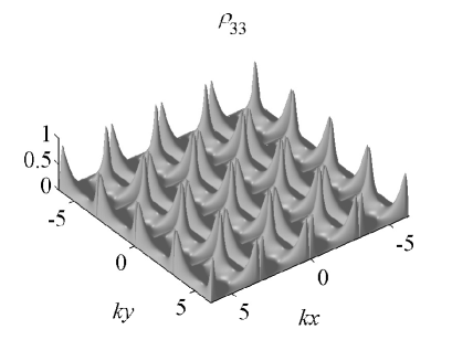
Figure 6: Spatial distribution of population in the $|3\rangle$ state under condition $\Delta_{1}\approx\Delta_{2}$. Peaks of the population are located near crossings of the nodal lines, width of the peaks is decreased by drawing near to CPT. The laser frequency detunings are $\Delta_{1}=10\gamma$, $\Delta_{2}=10.1\gamma$, $\Delta_{3}=15\gamma$; the Rabi frequencies of the standing waves are $G_{1}=G_{2}=5\gamma$, and the Rabi frequency of the probe running wave is $\Omega=0.3\gamma$. All other parameters are the same as in Fig. 2.

Localization of an atom can be performed by means of measuring the population whether in the upper state or in a ground state. These populations are defined by the atom-field interaction and they are rather different for each internal state. Therefore, we can choose not only parameters of the external fields, but we can also choose an internal level which is more suitable for measurement. In this section we analyze populations obtained numerically from Eqs. (6) in the long-time limit and demonstrate a high-precision localization due to measuring a ground-state population.

Distributions of the ground-state populations in a running-wave case of the probe field are shown in Fig. 4. Peaks of population in the $|1\rangle$ state occur at the nodes of standing wave $g_{1}(x)$ (see Fig. 4(a)), and peaks of population in state $|2\rangle$ occur at the nodes of standing wave $g_{2}(y)$ (see Fig. 4(b)). The atomic population at these peaks is concentrated in one ground state, so the atom can be localized much more easily than for the upper state. Population in the $|3\rangle$ state shown in Fig. 4(c) is avoided at the nodes of both standing waves, $g_{1}(x)$ and $g_{2}(y)$. Hence, in this way we have another type of localization when the atom due to absence of population can be localized at the nodes of both standing waves. Peaks of population along the $x$ axis have the width defined by the ratio of $\Omega/G_{1}$, while peaks of population along the $y$ axis have the width defined by the ratio of $\Omega/G_{2}$. The high-precision localization is obtained by means of decreasing the ratios of $\Omega/G_{1}$ and $\Omega/G_{2}$.

Let us consider a standing-wave case of the probe field. The width of the peaks along the $x$ direction can be decreased not only by means of the ratio of $\Omega/G_{1}$. In addition, the small width of the peaks is obtained when the nodes of the probe field are approximate to the nodes of standing wave $g_{1}(x)$, i.e. spatial phase shift $\psi\approx 0$. In the case of $\psi=0$ the peaks of the population in the $|1\rangle$ state are avoided, which leads to spatial structures of the population shown in Fig. 5. Distributions of the population take the forms similar to those of population in the upper state and can represent spikes, craters and waves. The heights of these structures are defined by the intensity $\Omega^{2}$ of the probe field.

Localization conditions discussed earlier correspond to large differences between the laser frequency detunings $\Delta_{1}$, $\Delta_{2}$ and $\Delta_{3}$. On the other hand, it is a well-known fact that in a tripod-like atom coherent population trapping (CPT) takes place when two of the laser detunings are equal. The 1D localization of an atom based on CPT has been demonstrated by Agarwal et al. Ag for a three-level $\Lambda$-type atom due to measurement of a ground-state population. Here we propose a way to carry out the 2D atom localization in a tripod-type atom under a condition close to CPT.

Let us consider the case of the running-wave probe field and $\Delta_{1}\approx\Delta_{2}$. While the atomic population under usual conditions is almost entirely in the $|3\rangle$ state, the atomic population in case of $\Delta_{1}=\Delta_{2}$ is trapped in the $|1\rangle$ and $|2\rangle$ states. So, when $\Delta_{1}\approx\Delta_{2}$ the behavior of the atomic populations rather differs from other cases and is of special interest. Note that the strong standing waves push out the atomic population from states $|1\rangle$ and $|2\rangle$ and hinder CPT, so intensities of the standing waves should be moderate. The distribution of population in the $|3\rangle$ state is shown in Fig. 6. Peaks of the population are located near crossings of the nodal lines. Width of the peaks is decreased by drawing near to CPT, and the high-precision localization is achieved for the small value of $|\Delta_{12}|$.

V Conclusion

In conclusion, we have presented a scheme for 2D subwavelength localization of a four-level tripod-like atom in laser fields. 2D spatial periodic structures of the upper-state population such as spikes, craters and waves are selected. The same structures are observed for population in ground state $|1\rangle$ in the case of $\psi=0$. Also, the atom observed in a ground state can be localized at the nodes of one of the standing waves. As a result, we have demonstrated methods having important practical applications in high-resolution atom lithography that are of particular interest because of the recent experiments for semiconductor elements Lee ; Chen ; Ind .

References

- (1) W. Heisenberg, Z. Phys. 43, 172 (1927).
- (2) P. Storey, M. J. Collett, and D. F. Walls, Phys. Rev. Lett. 68, 472 (1992).
- (3) P. Storey, M. J. Collett, and D. F. Walls, Phys. Rev. A 47, 405 (1993).
- (4) P. Storey, T. Sleator, M. J. Collett, and D. F. Walls, Phys. Rev. A 49, 2322 (1994).
- (5) S. Kunze, G. Rempe, and M. Wilkens, Europhys. Lett. 27, 115 (1994).
- (6) J. E. Thomas, Phys. Rev. A 42, 5652 (1990).
- (7) K. D. Stokes, C. Schnurr, J. R. Gardner, M. L. Marable, G. R. Welch, and J. E. Thomas, Phys. Rev. Lett. 67, 1997 (1991).
- (8) J. R. Gardner, M. L. Marable, G. R. Welch, and J. E. Thomas, Phys. Rev. Lett. 70, 3404 (1993).
- (9) R. Abfalterer, C. Keller, S. Bernet, M. K. Oberthaler, J. Schmiedmayer, and A. Zeilinger, Phys. Rev. A 56, R4365 (1997).
- (10) C. Keller, R. Abfalterer, S. Bernet, M. K. Oberthaler, J. Schmiedmayer, and A. Zeilinger, J. of Vac. Sci. Technol. B 16, 3850 (1998).
- (11) K. S. Johnson, J. H. Thywissen, N. H. Dekker, K. K. Berggren, A. P. Chu, R. Younkin, and M. Prentiss, Science 280, 1583 (1998).
- (12) A. M. Herkommer, W. P. Schleich, and M. S. Zubairy, J. Mod. Opt. 44, 2507 (1997).
- (13) S. Qamar, S.-Y. Zhu, and M. S. Zubairy, Opt. Commun. 176, 409 (2000).
- (14) S. Qamar, S.-Y. Zhu, and M. S. Zubairy, Phys. Rev. A 61, 063806 (2000).
- (15) F. Ghafoor, S. Qamar, and M. S. Zubairy, Phys. Rev. A 65, 043819 (2002).
- (16) E. Paspalakis and P. L. Knight, Phys. Rev. A 63, 065802 (2001).
- (17) E. Paspalakis, A. F. Terzis, and P. L. Knight, J. Mod. Opt. 52, 1685 (2005).
- (18) H. Theuer, R. G. Unanyan, C. Habscheid, K. Klein, and K. Bergmann, Opt. Express 4, 77 (1999).
- (19) F. Vewinger, M. Heinz, R. G. Fernandez, N. V. Vitanov, and K. Bergmann, Phys. Rev. Lett. 91, 213001 (2003).
- (20) P. Meystre and M. Sargent III, Elements of Quantum Optics, 3rd ed. (Springer-Verlag, Berlin, 1999).
- (21) G. S. Agarwal and K. T. Kapale, J. Phys. B: At. Mol. Opt. Phys. 39, 3437 (2006).
- (22) S. J. Rehse, K. M. Bockel, and S. A. Lee, Phys. Rev. A 69, 063404 (2004).
- (23) R. Chen, J. F. McCann, and I. Lane, J. Phys. B: At. Mol. Opt. Phys. 40, 1535 (2007).
- (24) B. Klöter, C. Weber, D. Haubrich, D. Meschede, and H. Metcalf, Phys. Rev. A 77, 033402 (2008).