Parametric Resonance in Bose-Einstein Condensates with Periodic Modulation of Attractive Interaction

Abstract

We demonstrate parametric resonance in Bose-Einstein condensates (BECs) with attractive two-body interaction in a harmonic trap under parametric excitation by periodic modulation of the s-wave scattering length. We obtain nonlinear equations of motion for the widths of the condensate using a Gaussian variational ansatz for the Gross-Pitaevskii condensate wave function. We conduct both linear and nonlinear stability analyses for the equations of motion and find qualitative agreement, thus concluding that the stability of two equilibrium widths of a BEC might be inverted by parametric excitation.

I Introduction

The phenomenon of parametric resonance, when a system is parametrically excited and oscillates at one of its resonant frequencies, is ubiquitous in physics: the phenomenon is found from simple classical systems such as the swing set and the vertically driven pendulum feynman , to the Paul ion trap paul and aspects of some inflation models of the universe kofman . Parametrically excited systems are frequently nonlinear: even the parametrically driven pendulum is governed by the linear Mathieu equation only for small oscillations about its equilibrium positions. Nonetheless, valuable qualitative insight into these systems may be gained by investigating their behavior in the vicinity of equilibrium points.

In the realm of ultracold quantum gases, studies of parametric resonance have featured Faraday patterns engels ; nicolin3 ; longhi ; nicolin1 ; capuzzi ; nicolin2 ; balaz ; balazneu , Kelvin waves of quantized vortex lines simula , self-trapped condensates ueda1 ; malomed1 , bright and vortex solitons ueda2 ; adhikari ; mueller1 , and self-damping at zero temperature kagan . Other investigations focus on the phenomenon of parametric resonance in the context of lower-dimensional Bose and Fermi gases graf ; mueller2 ; mueller3 . Parametric resonances have also been studied for optical lattices when the intensity of the lattice is periodically modulated in time dalfovo or when the lattice is shaken. In the latter case it was even shown that a periodic driving can induce a quantum phase transition from a Mott insulator to a superfluid holthaus ; arimondo , paving the way for new techniques to engineer exotic phases sengstock1 ; sengstock2 . Other novel experimental techniques malomed2 ; bagnato ; ramos to excite a Bose-Einstein condensate (BEC) of ⁷Li in the vicinity of a broad Feshbach resonance hulet by harmonic modulation of the $s$-wave scattering length, in contrast to the usual method of excitation by modulation of the trapping potential jin1 ; ketterle ; shlyapnikov ; jin2 ; torres ; abdullaev , have inspired investigations of parametric resonance and other phenomena in Refs. adhikari ; vidanovic ; rapp ; hamid . In the following we perform a systematic proof-of-concept study of the simplest case of parametric resonance in a three-dimensional BEC in a harmonic trap. To this end we demonstrate that within both a linear analytic and a nonlinear numeric analysis the stability characteristics of its equilibrium configurations can be changed by a periodic modulation of the attractive interaction.

II Variational Approach

We start with modeling the dynamics of a BEC at zero temperature using the mean-field Gross-Pitaevskii (GP) Lagrangian

$$L(t)=\int\bigg{[}\frac{i\hbar}{2}\left(\psi\frac{\partial\psi^{*}}{\partial t}-\psi^{*}\frac{\partial\psi}{\partial t}\right)-\frac{\hbar^{2}}{2m}|\nabla\psi|^{2}-V({\bf r})|\psi|^{2}-\frac{2\pi\hbar^{2}a(t)}{m}|\psi|^{4}\bigg{]}\,d{\bf r}.$$ (1)

Extremizing the Lagrangian results in the well-known GP equation for the dynamics of the mean-field condensate wave function $\psi=\psi({\bf r},t)$. In experiments generically a cylindrically-symmetric harmonic trapping potential $V({\bf r})=m\omega_{\rho}^{2}(\rho^{2}+\lambda^{2}z^{2})/2$ is used, whose elongation is described by the trap anisotropy parameter $\lambda=\omega_{z}/\omega_{\rho}$. Furthermore, we assume that the $s$-wave scattering length is periodically modulated according to

$$a(t)=a_{0}+a_{1}\sin{\Omega t}.$$ (2)

In the following we will investigate how the stability of condensate equilibria depends on both the driving amplitude $a_{1}$ and the driving frequency $\Omega$, provided the time-averaged $s$-wave scattering length $a_{0}$ is slightly negative. In principle, this could be analyzed by solving the underlying GP equation for the condensate wave function $\psi=\psi({\bf r},t)$, which follows from extremizing the Lagrangian (1). However, the thorough numerical analysis in Ref. vidanovic demonstrated convincingly that the dynamics of the GP equation can be well-approximated within a Gaussian variational ansatz for the GP condensate wave function zoller1 ; zoller2 . Even for long evolution times and in the vicinity of resonances, where oscillations of the condensate are quite large, it was possible to reduce the GP partial differential equation to a set of ordinary differential equations for the variational parameters.

Therefore, we follow the latter approach and employ the Gaussian ansatz

$$\psi^{\rm G}(\rho,z,t) = {\mathcal{N}}(t)\exp\left[-\frac{\rho^{2}}{2\tilde{u}_{\rho}^{2}}+i\rho^{2}\phi_{\rho}\right]\exp\left[-\frac{z^{2}}{2\tilde{u}_{z}^{2}}+iz^{2}\phi_{z}\right],$$ (3)

with time-dependent variational widths $\tilde{u}_{\rho}$, $\tilde{u}_{z}$, phases $\phi_{\rho}$, $\phi_{z}$, and normalization ${\mathcal{N}}(t)=N^{1/2}\pi^{3/2}{{\tilde{u}}_{\rho}}^{-1}{{\tilde{u}}_{z}}^{-1/2}.$ Inserting the Gaussian ansatz (3) into the GP Lagrangian (1) and extremizing with respect to all variational parameters, we obtain at first explicit expressions for the phases $\phi_{\rho,z}=m\dot{\tilde{u}}_{\rho,z}/(2\hbar{\tilde{u}}_{\rho,z})$. We define the dimensionless time $\tau=\omega_{\rho}t$ and scale the variational widths by $u_{\rho,z}={\tilde{u}}_{\rho,z}/a_{\rm ho}$, where $a_{\rm ho}=\sqrt{\hbar/(m\omega_{\rho})}$ is the harmonic oscillator length. Finally, we write the dimensionless driving function $p(\tau)=p_{0}+p_{1}\sin{\left(\Omega\tau/\omega_{\rho}\right)}$ according to the definitions $p_{0,1}=\sqrt{2/\pi}Na_{0,1}/a_{\rm ho}$. The resulting dynamics for the widths $u_{\rho}$ and $u_{z}$ is then determined by a pair of coupled nonlinear ordinary differential equations:

$$\ddot{u}_{\rho}+u_{\rho} = \frac{1}{u_{\rho}^{3}}+\frac{p(\tau)}{u_{\rho}^{3}u_{z}},$$

$$\ddot{u}_{z}+\lambda^{2}u_{z} = \frac{1}{u_{z}^{3}}+\frac{p(\tau)}{u_{\rho}^{2}u_{z}^{2}}.$$ (4)

For attractive two-body interactions, there is a critical value of the time-averaged interaction strength $p_{0}^{\rm crit}(\lambda)<0$ beyond which no equilibria exist in the absence of parametric driving. This means physically that for $p_{0}^{\rm crit}(\lambda)<0$ the BEC always collapses. The dependence of $p_{0}^{\rm crit}(\lambda)<0$ on the trap anisotropy $\lambda$ must be evaluated numerically, as for example in Ref. hamid . For $p_{0}^{\rm crit}(\lambda)<p_{0}<0$, there exists a pair of equilibrium points for Eqs. (4), one stable and one unstable zoller1 ; zoller2 , which we denote with ${\bf u}_{0+}$ and ${\bf u}_{0-}$, respectively. We remark that the stability of these points in the absence of parametric driving is determined by evaluating the frequencies of collective modes for small oscillations about equilibrium hamid . Whereas the equilibrium ${\bf u}_{0+}$ has real frequencies for all modes and is stable, the equilibrium ${\bf u}_{0-}$ possesses an imaginary frequency for one mode, implying exponential behaviour and thus instability.

III Linear Stability Analysis

In view of a linear stability analysis we assume small oscillations about an equilibrium, write $u_{\rho}\approx u_{\rho 0}+\delta u_{\rho}$ and $u_{z}\approx u_{z0}+\delta u_{\rho}$, and expand the nonlinear terms of Eqs. (4) to first order in $\delta u_{\rho}$ and $\delta u_{z}$. We scale and translate time as $2t^{\prime}+\pi/2=\Omega\tau/\omega_{\rho}$, define displacement and forcing vectors ${\bf x}(t^{\prime})$ and ${\bf f}$,

$${\bf x}(t^{\prime})=\left(\begin{array}[]{c}\delta u_{\rho}(\tau)\\ \delta u_{z}(\tau)\end{array}\right),\quad{\bf f}=4\left(\frac{\omega_{\rho}}{\Omega}\right)^{2}\left(\begin{array}[]{c}\frac{p_{1}}{u_{\rho 0}^{3}u_{z0}}\\ {\frac{p_{1}}{u_{\rho 0}^{2}u_{z0}^{2}}}\end{array}\right),$$ (9)

and finally we introduce the matrices ${\bf A}$ and ${\bf Q}$ corresponding to coefficients of constant and periodic terms, respectively:

$${\bf A} = 4\left(\frac{\omega_{\rho}}{\Omega}\right)^{2}\left(\begin{array}[]{cc}4&\frac{p_{0}}{u_{\rho 0}^{3}u_{z0}^{2}}\\ \frac{2p_{0}}{u_{\rho 0}^{3}u_{z0}^{2}}&3\lambda^{2}+\frac{1}{u_{z0}^{4}}\end{array}\right),$$ (12)

$${\bf Q} = -2\left(\frac{\omega_{\rho}}{\Omega}\right)^{2}\left(\begin{array}[]{cc}{\frac{3}{u_{\rho 0}^{4}{u_{z0}}}}&{\frac{1}{u_{\rho 0}^{3}u_{z0}^{2}}}\\ {\frac{2}{u_{\rho 0}^{3}u_{z0}^{2}}}&{\frac{2}{u_{\rho 0}^{2}u_{z0}^{3}}}\end{array}\right).$$ (15)

The result consists of two coupled inhomogeneous Mathieu equations

$$\ddot{\bf x}(t^{\prime})+\left({\bf A}-2p_{1}{\bf Q}\cos{2t^{\prime}}\right){\bf x}(t^{\prime})={\bf f}\cos{2t}^{\prime},$$ (16)

whose solutions determine whether the underlying equilibrium is stable or unstable.

The Mathieu equation, a special case of Hill’s differential equation stegun , has been studied extensively in the literature mclachlan . Approaches to obtaining its stability diagram include continued fractions stegun ; risken ; simmendinger , perturbative methods nayfeh ; younesian ; mahmoud , and infinite determinant methods lindh ; pedersen ; hansen ; landa . The problem has been treated in detail in Ref. ozakin for the study of the Paul trap, the stability of which is governed exactly by a set of coupled homogeneous Mathieu equations. Of importance to our particular problem are Refs. kotowski ; slane , where it was shown that for both single and coupled Mathieu equations, a harmonic inhomogeneous term does not affect the location of stability borders to Eq. (16).

In many approaches (see, for example, Ref. landa ), Eq. (16) is reformulated as a first-order non-autonomous Floquet system

$$\dot{\phi}={\bf G}(t^{\prime})\phi,$$ (17)

where $\phi=\left[{\bf x}\;\;{\bf\dot{x}}\right]^{T}$, and

$${\bf G}(t^{\prime})=\left(\begin{array}[]{cc}{\bf 0}&{\bf 1}_{2}\\ -\left({\bf A}-2p_{1}{\bf Q}\cos{2t^{\prime}}\right)&{\bf 0}\end{array}\right)$$ (18)

is $\pi$-periodic. Linearly independent solutions to the Floquet problem may be written as a fundamental matrix solution $\Phi(t^{\prime})$ with the initial condition $\Phi(0)={\bf 1}_{4}$:

$$\dot{\Phi}(t^{\prime})={\bf G}(t^{\prime})\,\Phi(t^{\prime}).$$ (19)

It can be shown that solutions to Eq. (19) are stable if the eigenvalues $\lambda_{n}$ of $\Phi(t^{\prime}=\pi)$ satisfy $|\lambda_{n}|\leq 1$. Further, we define characteristic exponents $\beta_{n}$ such that $\lambda_{n}=e^{\beta_{n}\pi}$, with the result that stable solutions ${\bf x}_{1,2}(t^{\prime})$ to Eq. (16) may be written in the form yakubovich

$${\bf x}_{1,2}(t^{\prime})=e^{\pm\beta t^{\prime}}\sum_{n=-\infty}^{\infty}{\bf b}_{2n}e^{2int^{\prime}}.$$ (20)

On the stability borders, Eq. (20) provides one linearly independent solution that is periodic; a second is non-periodic and grows linearly with time. In constructing the linear stability diagram, we use two complementary approaches: a matrix continued fraction approach based on Refs. risken ; simmendinger determines the stability borders analytically, while a numerical integration of Eq. (19) to obtain the characteristic multipliers $\lambda_{n}$ determines the stable or unstable character of the respective diagram regions.

By substitution of the Floquet ansatz (20) into Eq. (16), we obtain a third-order recurrence relation for the Fourier coefficients ${\bf b}_{2n}$:

$$\left[{\bf A}+\left(\beta+2in\right)^{2}{\bf I}\right]{\bf b}_{2n}-p_{1}{\bf Q}\left({\bf b}_{2n+2}+{\bf b}_{2n-2}\right)=\bf 0.$$ (21)

We define the ladder operators ${\bf S}_{2n}^{\pm}{\bf b}_{2n}={\bf b}_{2n\pm 2}$ as

$${\bf S}_{2n}^{\pm}=\left\{{\bf A}+\left[\beta+2i\left(n+1\right)\right]^{2}{\bf I}-p_{1}{\bf Q}{\bf S}_{2n\pm 2}^{\pm}\right\}^{-1}p_{1}{\bf Q},$$ (22)

and by repeated re-substitution of these ladder operators into the recursion relation (21) for $n$ increasing and decreasing from zero, we obtain a tri-diagonal matrix-valued continued fraction relating the parameters ${\bf A}$, ${\bf Q}$, and $\beta$:

$${\bf\bigg{(}}{\bf A}+\beta^{2}{\bf I}-p_{1}^{2}{\bf Q}\bigg{\{}\left[{\bf A}+\left(\beta+2i\right)^{2}{\bf I}-\dots\right]^{-1}+\left[{\bf A}+\left(\beta-2i\right)^{2}{\bf I}-\dots\right]^{-1}\bigg{\}}{\bf Q}{\bf\bigg{)}}{\bf b}_{0}=\bf 0.$$ (23)

In order to obtain a non-trivial solution for ${\bf b}_{0}$, the determinant of the matrix-valued continued fraction (23) must vanish. Since on the stability borders one linearly independent solution is periodic, it suffices to set $\beta=\{0,\pm i\}$ in Eq. (23) and truncate the continued matrix inversion, determining the stability borders in terms of the dimensionless driving amplitude $p_{1}$ and the driving frequency $\Omega$. Empirically, a truncation at ${\bf S}_{4}^{\pm}$ proves to be sufficient for accurate results. The resulting stability for particular values of $\Omega$ and $p_{1}$ is then shown in the linear stability diagram of Fig. 1 for three characteristic values of the trap anisotropy $\lambda$. Our results indicate that for the unstable (stable) equilibrium position, the largest region of stability (instability) occurs for a pancake-shaped BEC, i.e., for $\lambda>1$.

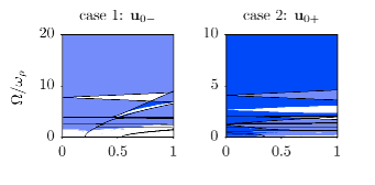
(a)

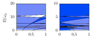
(b)

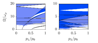
(c)

Figure 1: Linear stability diagrams from solving two coupled Mathieu equations for the unstable (case 1) and stable (case 2) equilibrium positions of a cylindrically-symmetric BEC for three values of the trap anisotropy $\lambda$: (a) $\lambda=0.2$ (a cigar-shaped BEC), (b) $\lambda=1$ (spherical BEC), and (c) $\lambda=2.6$ (pancake-shaped BEC). White regions correspond to unstable solutions, darkest shaded regions to stable solutions, and lightly shaded regions correspond to marginally stable solutions – regions where only one of two available collective oscillation modes is stable.

As a special case the stability borders for the isotropic condensate follow from the 3D spherically symmetric version of Eq. (3) and are given by a separate continued fraction, obtained by an analogous process for a single inhomogeneous Mathieu equation. The resulting stability diagrams are shown in Fig. 2. The isotropic case allows a direct analogy between the condensate and the parametrically driven pendulum: the pendulum too is described by a single Mathieu equation, however the inhomogeneous term in the equation of motion for the BEC corresponds to a direct periodic driving in phase with the parametric driving. It was shown in Ref. kotowski that a periodic inhomogeneity has no effect on the stability borders for a single Mathieu equation, so Fig. 2 is simply a transformation of the standard Ince-Strutt stability diagram for the parametrically driven pendulum stegun , for the relevant experimental parameters of the BEC.

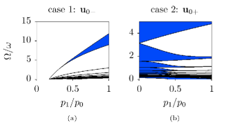
Figure 2: Linear stability diagrams from solving a single Mathieu equation for (a) unstable and (b) stable equilibria of a 3D spherically symmetric BEC. Shaded and white regions indicate stable and unstable solutions, respectively. The presence of a stable region in (a) indicates that an originally unstable equilibrium might be stabilized by parametric excitation.

While the results of linear stability analysis for the coupled Mathieu system are qualitatively similar to those for the single equation, there are a number of notable changes between Figs. 1 and 2. First, for the coupled Mathieu equations, there exist a set of stability regions not attainable by the analytic method used here. These are displayed without black borders in Fig. 1, and correspond to the so-called “combined resonances” of the system hansen ; ozakin . These regions are attainable by numerical stability analysis of the Mathieu equations yakubovich ; ozakin ; syranian , which was used to generate the colored background regions of Fig. 1. It is notable in Fig. 1 that these anomalous regions are not present for $\lambda=1$.

A second and important difference from the single to the coupled Mathieu equations is the appearance of a new region, shaded white and issuing from $\Omega/\omega_{\rho}\approx 10$ in Fig. 1 for $\lambda=1$, case 1. This region is identified with the instability of the quadrupole collective mode, which does not appear in a one-dimensional analysis. This result implies that a three-dimensional analysis might result in further changes to the linear stability diagram of Fig. 1 for $\lambda=1$, case 1.

IV Nonlinear Numerics

As the underlying equations of motion (4) are inherently nonlinear, a linear analytic stability analysis alone is not sufficient to fully investigate the phenomenon of parametric resonance. Therefore, we have also performed a detailed numerical stability analysis by integrating the equations of motion (4) over a long time-period using a Runge-Kutta-Verner 8(9) order algorithm, incrementing through pairs $(p_{1},\Omega)$ and recording divergent solutions to obtain the corresponding stability diagram. The corresponding results are shown in Fig. 3 for the same three values of the trap anisotropy $\lambda$ as in Fig. 1.

The results for the originally stable equilibrium ${\bf u}_{0+}$ show both qualitative and even quantitative similarity to the linear stability analysis of Fig. 1, i.e., a similar tonguelike structure of unstable regions issuing from certain points on the vertical axis. The originally unstable equilibrium ${\bf u}_{0-}$ also shows qualitative similarity to the linear analysis of Fig. 1, however the region of stability begins only for much larger modulation frequency $\Omega$ and dimensionless driving amplitude $p_{1}$. These results are both reasonable, as the linear stability analysis is only valid for small oscillations – corresponding to large $(p_{1},\Omega)$ for equilibrium ${\bf u}_{0+}$ and small $(p_{1},\Omega)$ for equilibrium ${\bf u}_{0-}$. Furthermore, in contrast to Fig. 1, we find in the nonlinear stability diagram of Fig. 3 that stability is more easily achieved for a cigar-shaped BEC, i.e., for $\lambda<1$.

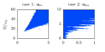
(a)

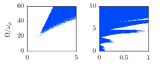
(b)

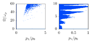
(c)

Figure 3: Nonlinear stability diagrams for the unstable (left) and stable (right) equilibria of a cylindrically-symmetric BEC, for three values of the trap anisotropy $\lambda$: (a) $\lambda=0.2$ (a cigar-shaped BEC), (b) $\lambda=1$ (spherical BEC), and (c) $\lambda=2.6$ (pancake-shaped BEC). Shaded and white regions indicate stable and unstable solutions, respectively.

Further comparison of the linear and nonlinear stability diagrams of Figs. 1 and 3 shows the possibility of both simultaneous stability of the equilibrium positions, and even the possibility of a complete reversal of the stability characteristics. In the latter case, the smaller equilibrium position would become the only stable width of the condensate, which should be experimentally observable. A final observation, applicable to the originally unstable equilibrium in both linear and nonlinear cases, is the existence of a minimum driving amplitude $p_{1}^{\rm min}$ necessary to stabilize the condensate. The value $p_{1}^{\rm min}=u_{0}(5u_{0}^{4}-1)\approx 0.17~{}p_{0}$ is exactly attainable for the linear analysis of the isotropic condensate, and in Fig. 1 is approximately independent of $\lambda$ in the considered range [0.2,2.6]. For the nonlinear analysis, $p_{1}^{\rm min}\approx 1.2~{}p_{0}$ is also approximately independent of $\lambda$. This feature will have implications for an experiment, as in conjunction with the width of the Feshbach resonance, it dictates the minimum modulation of the applied magnetic field necessary to stabilize the condensate.

We note that any stability diagram depends on the particular choice for the time-averaged dimensionless interaction strength $p_{0}$. The concrete results in Figs. 1–3 were obtained for the particular value $p_{0}=0.9~{}p_{0}^{\rm crit}(\lambda)$. As $p_{0}$ approaches $p_{0}^{\rm crit}(\lambda)$, we generically observe a growth of the stable (unstable) regions in case 1 (2).

V Conclusions

Finally, we conclude that our proof-of-concept investigation has unambiguously shown that the phenomenon of parametric resonance should also be experimentally observable in terms of changed stabilities for the equilibrium configurations of a three-dimensional BEC in a harmonic trap with a periodic modulation of the attractive interaction. However, due to the intrinsic nonlinear nature of the underlying GP mean-field theory, a linear analysis, like in the Paul trap, is not sufficient to quantitatively study the stability diagram. Thus, in order to achieve a destabilization (stabilization) of a stable (unstable) BEC equilibrium in an experiment, a corresponding numerical nonlinear analysis is indispensable. Regardless, a linear stability analysis provides an intuitive and qualitative understanding of the physics of parametric resonance in BECs.

In the present letter we have focused our attention upon a periodic modulation of the $s$-wave scattering length around a slightly negative value, which restricts the number of particles in a BEC to the order of a few thousand bradley ; bradleyerrata . However, the phenomenon of parametric resonance might be more important for dipolar BECs, where in addition to a repulsive short-range and isotropic interaction, also a long-range and anisotropic dipolar interaction between atomic magnetic or molecular dipoles is present. Provided that the dipolar interaction is smaller than the contact interaction, a stable dipolar BEC does exist. But a larger dipolar strength leads to mutual existence of both a stable and an unstable dipolar BEC eberlein whose stability might be changed via a periodic modulation of the harmonic trap frequencies or the $s$-wave scattering length. In that context it might also be of interest to estimate how quantum fluctuations, which are non-negligible for a larger dipolar interaction strength lima1 ; lima2 , change the stability diagram. The case for dipolar Fermi gases is probably even more interesting from the point of view of parametric resonance, as for any dipolar strength a stable equilibrium coexists with an unstable one lima3 ; lima4 . Thus, parametric resonance may offer a simple efficient approach for realizing equilibria of dipolar quantum gases whose properties have so far not yet been explored.

References

References

- (1) R. P. Feynman, R. B. Leighton, and M. Sands, The Feynman Lectures on Physics, Vol. 1 (Addison-Wesley, New York, 1964).
- (2) W. Paul, Angew. Chem. Int. Ed. Engl. 29, 739 (1990).
- (3) L. Kofman, A. Linde and A. A. Starobinsky, Phys. Rev. Lett. 73, 3195 (1994).
- (4) P. Engels, C. Atherton, and M. A. Hoefer, Phys. Rev. Lett. 98, 095301 (2007).
- (5) A. I. Nicolin, R. Carretero-Gonzalez, and P. G. Kevrekidis, Phys. Rev. A 76, 063609 (2007).
- (6) K. Staliunas, S. Longhi, and G.J. de Valcárcel, Phys. Rev. Lett. 89, 210406 (2002).
- (7) A. I. Nicolin, Phys. Rev. E 84, 056202 (2011).
- (8) P. Capuzzi, M. Gattobigio, and P. Vignolo, Phys. Rev. A 83, 013603 (2011).
- (9) A. I. Nicolin, Physica A 391, 1062 (2012).
- (10) A. Balaž and A. I. Nicolin, Phys. Rev. A 85, 023613 (2012).
- (11) A. Balaž, R. Paun, A.I. Nicolin, S. Balasubramanian, and R. Ramaswamy, Phys. Rev. A 89, 023609 (2014).
- (12) T. P. Simula, T. Mizushima, and K. Machida, Phys. Rev. Lett. 101, 020402 (2008).
- (13) H. Saito, R. G. Hulet, and M. Ueda, Phys. Rev. A 76, 053619 (2007).
- (14) F. Kh. Abdullaev, J. G. Caputo, R. A. Kraenkel, and B. A. Malomed, Phys. Rev. A 67, 013605 (2003).
- (15) H. Saito and M. Ueda, Phys. Rev. Lett. 90, 040403 (2003).
- (16) S. K. Adhikari, Phys. Rev. A 69, 063613 (2004).
- (17) C. Gaul, E. Díaz, R. P. A. Lima, F. Domínguez-Adame, and C. A. Müller, Phys. Rev. A 84, 053627 (2011)
- (18) Y. Kagan and L. A. Maksimov, Phys. Rev. A 64, 053610 (2001).
- (19) C. D. Graf, G. Weick, and E. Mariani, EPL 89, 40005 (2010)
- (20) E. Díaz, C. Gaul, R. P. A. Lima, F. Domínguez-Adame, and C. A. Müller, Phys. Rev. A 81, 051607(R) (2010)
- (21) C. Gaul, R. P. A. Lima, E. Díaz, C. A. Müller, and F. Domínguez-Adame, Phys. Rev. Lett. 102, 255303 (2009)
- (22) C. Tozzo, M. Krämer, and F. Dalfovo, Phys. Rev. A 72, 023613 (2005).
- (23) A. Eckardt, C. Weiss, and M. Holthaus, Phys. Rev. Lett. 95, 260404 (2005).
- (24) A. Zenesini, H. Lignier, D. Ciampini, O. Morsch, and E. Arimondo, Phys. Rev. Lett. 102, 100403 (2009).
- (25) J. Struck, C. Olschlager, R. Le Targat, P. Soltan-Panahi, A. Eckardt, M. Lewenstein, P. Windpassinger, and K. Sengstock, Science 333, 996 (2011).
- (26) J. Struck, C. Olschlager, M. Weinberg, P. Hauke, J. Simonet, A. Eckardt, M. Lewenstein, K. Sengstock, and P. Windpassinger, Phys. Rev. Lett. 108, 225304 (2012).
- (27) E. R. F. Ramos, E. A. L. Henn, J. A. Seman, M. A. Caracanhas, K. M. F. Magalhães, K. Helmerson, V. I. Yukalov, and V. S. Bagnato, Phys. Rev. A 78, 063412 (2008).
- (28) P. G. Kevrekidis, G. Theocharis, D. J. Frantzeskakis, and B. A. Malomed, Phys. Rev. Lett. 90, 230401 (2003).
- (29) S. E. Pollack, D. Dries, R.G. Hulet, K.M.F. Magalhães, E.A.L. Henn, E.R.F. Ramos, M.A. Caracanhas, and V.S. Bagnato, Phys. Rev. A 81, 053627 (2010).
- (30) S. E. Pollack, D. Dries, M. Junker, Y. P. Chen, T. A. Corcovilos, and R. G. Hulet, Phys. Rev. Lett. 102, 090402 (2009).
- (31) D. S. Jin, J. R. Ensher, M. R. Matthews, C. E. Wieman, and E. A. Cornell, Phys. Rev. Lett. 77, 420 (1996).
- (32) M.-O. Mewes, M. R. Andrews, N. J. van Druten, D. M. Kurn, D. S. Durfee, and W. Ketterle, Phys. Rev. Lett. 77, 416 (1996).
- (33) Yu. Kagan, E. L. Surkov, and G. V. Shlyapnikov, Phys. Rev. A 54, R1753 (1996).
- (34) D. S. Jin, M. R. Matthews, J. R. Ensher, C. E. Wieman, and E. A. Cornell, Phys. Rev. Lett. 78, 764 (1997).
- (35) J. J. García-Ripoll, V. M. Pérez-García, and P. Torres, Phys. Rev. Lett. 83, 1715 (1999).
- (36) F. Kh. Abdullaev and J. Garnier, Phys. Rev. A 70, 053604 (2004)
- (37) I. Vidanovic, A. Balaž, H. Al-Jibbouri, and A. Pelster, Phys. Rev. A 84, 013618 (2011).
- (38) A. Rapp, X. Deng, and L. Santos, Phys. Rev. Lett. 109, 203005 (2012).
- (39) H. Al-Jibbouri, I. Vidanovic, A. Balaž, and A. Pelster, J. Phys. B 46, 065303 (2013).
- (40) V. M. Pérez-García, H. Michinel, J. I. Cirac, M. Lewenstein, and P. Zoller, Phys. Rev. Lett. 77, 5320 (1996).
- (41) V. M. Pérez-García, H. Michinel, J. I. Cirac, M. Lewenstein, and P. Zoller, Phys. Rev. A 56, 1424 (1997).
- (42) M. Abramowitz and I. A. Stegun, Handbook of Mathematical Functions with Formulas, Graphs and Mathematical Tables (Dover, New York, 1972).
- (43) N. W. McLachlan, Theory and Applications of Mathieu Functions (Oxford, Clarendon, 1947).
- (44) H. Risken, The Fokker-Planck Equation (Springer, Berlin, 1989).
- (45) C. Simmendinger, A. Wunderlin, and A. Pelster, Phys. Rev. E 59, 5344 (1999).
- (46) A. H. Nayfeh, Perturbation Methods (Wiley-VCH, Weinheim, 2004).
- (47) D. Younesian, E. Esmailzadeh, and R. Sedaghati, Commun. Nonlinear Sci. Numer. Simul. 12, 58 (2007).
- (48) G. M. Mahmoud, Physica A 242, 239 (1997).
- (49) K. G. Lindh, Am. Inst. Aer. Astr. J. 8, 680 (1970).
- (50) P. Pedersen, Ingenieur-Archiv 49, 15 (1980).
- (51) J. Hansen, Ingenieur-Archiv 55, 463 (1985).
- (52) H. Landa, M. Drewsen, B. Reznik, and A. Retzker, J. Phys. A: Math. Theor. 45, 455305 (2012)
- (53) A. Ozakin and F. Shaikh, J. Appl. Phys. 112, 074904 (2012).
- (54) G. Kotowski, Z. Angew. Math. Mech. 23, 213 (1943).
- (55) J. Slane and S. Tragesser, Nonlin. Dyn. Syst. Th. 11, 183 (2011).
- (56) V. A. Yakubovich and V.M. Starzhinski, Linear differential equations with periodic coefficients (Wiley, New York, 1975).
- (57) A. A. Mailybaev, O. N. Kirillov, and A. P. Seyranian, J. of Phys. A: Math. 38, 1723 (2005).
- (58) C. C. Bradley, C. A. Sackett, J. J. Tollett, and R. G. Hulet, Phys. Rev. Lett. 75, 1687 (1995).
- (59) C. C. Bradley, C. A. Sackett, J. J. Tollett, and R. G. Hulet, Phys. Rev. Lett. 79, 1170 (1997).
- (60) D. H. J. O’Dell, S. Giovanazzi, and C. Eberlein, Phys. Rev. Lett. 92, 250401 (2004).
- (61) A. R. P. Lima and A. Pelster, Phys. Rev. A 84, 041604(R) (2011).
- (62) A. R. P. Lima and A. Pelster, Phys. Rev. A 86, 063609 (2012).
- (63) A. R. P. Lima and A. Pelster, Phys. Rev. A 81, 021606(R) (2010).
- (64) A. R. P. Lima and A. Pelster, Phys. Rev. A 81, 063629 (2010).