Simulation of stochastic quantum systems using polynomial chaos expansions

Abstract

We present an approach to the simulation of quantum systems driven by classical stochastic processes that is based on the polynomial chaos expansion, a well-known technique in the field of uncertainty quantification. The polynomial chaos expansion represents the system density matrix as a series of orthogonal polynomials in the principle components of the stochastic process and yields a sparsely coupled hierarchy of linear differential equations. We provide practical heuristics for truncating this expansion based on results from time-dependent perturbation theory and demonstrate, via an experimentally relevant one-qubit numerical example, that our technique can be significantly more computationally efficient than Monte Carlo simulation.

I Introduction

Quantitative understanding of the dynamics of open quantum systems is critically important to many contemporary physics experiments Breuer02a . While the equations of motion for open systems models are often simple to formulate, in only a few special cases may they be solved analytically, and numerical studies are often limited to small systems. However, when quantum back action can be neglected, i.e., at high temperature or for short times, fully quantum open systems may be well approximated by semi-classical stochastic driving, whereupon the environment interaction operators are replaced by classical stochastic processes. For example, the coherence decay of diamond nitrogen-vacancy (NV) centers in the presence of dilute paramagnetic defects may be modeled very well by assuming that paramagnetic defects in the lattice produce a classical, fluctuating Overhauser field which dephases the NV center Hanson08a ; Ladd10a . Expensive numerical studies modeling the full quantum environment are then only required only to determine the statistical properties of this effective field. The resulting stochastic models are often sufficient to compute any desired system observables. However, these reduced models exchange quantum degrees of freedom for stochastic ones that may also require large, but significantly reduced, computational overhead. Expectation values of the system observables may then, in principle, be computed by averaging over the stochastic degrees of freedom in a manner that is consistent with the statistics of the stochastic process. In practice, however, such an average is often difficult to calculate. Monte Carlo (MC) methods Press92a approximate this average by generating many sample noise trajectories, integrating the Schrödinger equation for each trajectory, and averaging the resulting density operators. However, MC can be notoriously slow to converge, making it impractical for applications requiring iterative numerical calculations, such as optimal control Grace07a ; *Grace07b; Gorman12a . Perturbative master equations, on the other hand, are often either computationally inexpensive and inaccurate, or expensive and accurate, depending on the approximations made in their derivation Breuer02a .

In this work, we present an alternative approach to performing the stochastic average based on a class of techniques used widely in classical uncertainty quantification. Known as the polynomial chaos expansion (PCE) Debusschere04a ; LeMaitre10a , this method leverages properties of orthogonal polynomials to yield a converging sequence of approximate evolution equations for a quantum system undergoing stochastic driving without resorting to MC methods. While we restrict our discussion to quantum systems driven by classical Gaussian stochastic processes, we make no assumptions of weak coupling nor do we restrict the form of the noise correlation function. Furthermore, we show that the linearity of the Schrödinger equation makes quantum systems particularly well suited to the PCE approach, as the stochastic dynamics may be expressed in terms of a sparsely-coupled system of differential equations.

We begin this article with a derivation of Karhunen-Loéve decomposition, which expresses correlated, classical stochastic processes as an easily truncated sum of deterministic functions weighted by uncorrelated random variables. We proceed to use this decomposition to derive the PCE as applied to stochastic quantum systems, yielding a sparsely-coupled system of Schrödinger-like equations. We conclude with a discussion and numerical simulation of the convergence properties of this method, benchmarking our results against Monte Carlo simulations.

II Model

We consider a quantum two-level system coupled linearly to a classical stochastic process, $\Omega$, and described by the Hamiltonian, $H(t;\Omega(t))=H_{0}(t)+\Omega(t)V$. Switching to a rotating frame with respect to $H_{0}$, we obtain:

$$\tilde{H}(t;\Omega(t))=\Omega(t)U_{0}(t)^{\dagger}VU_{0}\equiv\Omega(t)\tilde{V}(t),$$ (1)

where $U_{0}=\underset{\leftarrow}{\mathcal{T}}\exp(-i\int_{0}^{t}H_{0}(s)ds)$ and $\underset{\leftarrow}{\mathcal{T}}$ is the Dyson time-ordering operator. Hamiltonians of this form are quite common, and restriction to this minimal form simplifies the following derivations. Generalizations to multiple or more complicated dependence on the stochastic process require only straightforward modifications to the following procedure.

We restrict our discussion here to stochastic processes, $\Omega$, which are mean-zero, Gaussian, and stationary Ripley08 . By Wick’s theorem Gardiner04b , such processes may be completely described in terms of their two-point correlation functions, $C(t_{1},t_{2})\equiv\left\langle{\Omega(t_{1})\Omega(t_{2})}\right\rangle_{\Omega}$. In this article, we use the notation $\left\langle{f(\Omega(t))}\right\rangle_{\Omega}$ to signify the expectation value of the function $f$ with respect to the process, $\Omega$.

The state of the system when conditioned on a specific realization of the stochastic process, $\rho(t;\{\Omega(t)\})$, will evolve according to the Schrödinger–von Neumann equation:

$$i\frac{d\rho(t;\{\Omega(t)\})}{dt}=\Omega(t)V(t)^{\times}\rho(t;\{\Omega(t)\}),$$ (2)

where we have used the superoperator adjoint notation $A^{\times}B=[A,B]$. At a time $\tau$, the state of the system, averaged over the stochastic process, is given by the formal expression

$$\rho(\tau)=\left\langle{U(\tau;\{\Omega(t)\})\rho(0)U(\tau;\{\Omega(t)\})}\right\rangle_{\Omega},$$ (3)

where $U(\tau;\{\Omega(t)\})$ denotes the unitary operator generated by Eq. (2) with a specific realization of $\Omega$. The objective of this work is to demonstrate that this stochastic average may be performed in a computationally efficient manner using the PCE.

II.1 Karhunen-Loéve Expansion

If the stochastic process, $\Omega$, is white, the average in Eq. (3) may be taken locally in time, and the system dynamics may be described exactly by a Lindblad master equation Breuer02a . However, the presence of non-vanishing time correlations greatly complicates the calculation of the stochastic average. To simplify this calculation, we employ the Karhunen-Loéve expansion (KLE) LeMaitre10a , which expresses a continuous, correlated process in terms of a discrete sum of deterministic functions weighted by uncorrelated random-variables:

$$\Omega(t)=\sum_{n=1}^{\infty}\sqrt{\lambda_{n}}g_{n}(t)\xi_{n}.$$ (4)

Here, $\xi_{n}\in\mathcal{N}(0,1)$ are independent and identically distributed (iid) random variables drawn from a unit-variance, zero-mean Gaussian distribution, while $\lambda_{n}$ and $g_{n}(t)$ are, respectively, the eigenvalues and $L_{2}$-orthonormal eigenfunctions of the Fredholm equation LeMaitre10a :

$$\int_{0}^{\tau}C(t_{1},t_{2})g_{n}(t_{2})dt_{2}=\lambda_{n}g_{n}(t_{1}).$$ (5)

Here, the correlation function acts as a symmetric, positive semi-definite integral kernel, so Mercer’s theorem LeMaitre10a implies that the eigenvalues, $\lambda_{n}$, are discrete and non-negative. Non-negativity is ensured because the correlation functions of stationary processes are positive semi-definite (by Bochner’s theorem Reed80a ), while discreteness is guaranteed by the finite upper limit on the integral, Eq. (5).

Interestingly, when the final time is much greater than the correlation time of the stochastic process, i.e., $\tau\gg\tau_{c}$, the Wiener-Khinchin theorem Gardiner04b implies that the eigenvalue spectrum becomes continuous and equal to the noise power spectral density, i.e., $\lambda_{\omega}=S(\omega)$, while the eigenfunctions take the form $g_{\omega}(t)\propto\cos(\omega t)$. Taken to the extreme white-noise limit, where $\tau_{c}\rightarrow 0$, all eigenvalues are equal. In the regime where $\tau\rightarrow\tau_{c}$, the correlation function is approximately constant over the integration window, and the Fredholm equation possesses only a single nonzero eigenvalue, with eigenfunction $g_{1}(t)\propto 1$. In this case, the stochastic process may be well approximated as a random variable which is constant over $t\in[0,\tau]$. Figure 1 illustrates these two limits by plotting the eigensystem of the Fredholm equation for Orenstein-Uhlenbeck Gardiner04b noise with two different decay parameters.

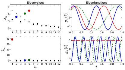
Figure 1: (color online) The eigenvalues, $\lambda_{n}$ (left, gray $\times$’s); cumulative transition rates, $\Gamma_{n}$, (left, solid circles); and eigenfunctions, $g_{n}(t)$ (right), of the Fredholm equation, Eq. (5), for Orenstein-Uhlenbeck noise, where $C(t)=\exp(-\left|t\right|/\tau_{c})$, calculated with final time $\tau=1$ and Hamiltonian $H(t)=B\sigma_{x}+\Omega(t)\sigma_{z}$. The top row corresponds to noise correlation time $\tau_{c}=0.1$ and magnetic field $B=5$, while the bottom row for $\tau_{c}=10$ and magnetic field $B=20$. The stochastic modes with the three largest transition rates are color coordinated with the eigenfunction plots (in descending transition rates: red dot and long dashed line; green dot and short dashed line; blue dot and solid blue line). For long correlation times, compared to $\tau$, only one mode is dominant, while more modes are increasingly important for shorter correlation times.

When the correlation time is relatively long compared to the evolution time, but not infinite, e.g., when $\tau<\tau_{c}$, the expansion Eq. (4) is dominated by only a few terms corresponding to the largest $S$ eigenvalues, and so may be truncated with minimal error. However, truncating the KLE based only on the eigenvalues ignores the impact that higher frequency modes could have on the dynamics, e.g.,, resonance. We therefore propose a more physically motivated truncation criterion based on results from time-dependent perturbation theory Sakurai94a . For static Hamiltonian terms $H_{0}$ and $V$ in the Schrödinger picture, the rate at which any given mode, $g_{n}(t)$, could cause a transition between the $j$th and $k$th eigenstates of $H_{0}$ is given by

$$\Gamma_{n}^{jk}=\frac{1}{\tau}\left|\left\langle j\left|V\right|k\right\rangle\int_{0}^{\tau}e^{i(E_{j}-E_{k})t}\sqrt{\lambda_{n}}g_{n}(t)dt\right|^{2},$$ (6)

where $H_{0}|j\rangle=E_{j}|j\rangle$. Summing over these eigenstates provides a measure of the degree to which a given mode will impact the evolution of the system, i.e., the cumulative transition rate, $\Gamma_{n}=\sum_{j,k}\Gamma_{n}^{jk}$. In addition to the eigenvalues, $\lambda_{n}$, and eigenfunctions, $g_{n}(t)$, of the Fredholm equation, Eq. (5), cumulative transition rates are also included in Figure 1. Thus, we approximate the expansion Eq. (4) by keeping only those modes corresponding to the $S$ largest transition rates, $\Gamma_{n}$; we shall refer to $S$ as the stochastic dimension. With this approximation, Eq. (2) becomes

$$i\frac{d\rho(t;\vec{\xi})}{dt}=\sum_{n=1}^{S}\sqrt{\lambda_{n}}g_{n}(t)\xi_{n}V(t)^{\times}\rho(t;\vec{\xi}).$$ (7)

We emphasize that this truncation strategy differs from that usually taken in standard uncertainty quantification literature LeMaitre10a , wherein the truncation is based on the magnitude of the eigenvalues alone, and without consideration to the potential impact of a given stochastic mode on the system dynamics.

II.2 Expansion in orthogonal polynomials

At the final time, $\tau$, the state of the system may be considered as a complicated function of the $S$ uncorrelated random variables from Eq. (4), i.e., $\rho(\tau)=\rho(\tau;\vec{\xi})$, as expressed in Eq. (7). As such, we may expand this function in a complete basis of orthogonal polynomials, $\Phi_{n}(\vec{\xi})$:

$$\rho(t;\vec{\xi})=\sum_{n=0}^{\infty}\phi_{n}(t)\Phi_{n}(\vec{\xi}\,),$$ (8)

yielding the (untruncated) PCE. Here, $\phi_{n}(t)$ are the time-dependent, operator-valued expansion coefficients that represent our new dynamical variables. The polynomials should be orthogonal under the measure, $\mu d\xi=\exp(-\xi^{2}/2)/\sqrt{2\pi}d\xi$, which is derived from the stationary distribution of the random variables, which are drawn from $\mathcal{N}(0,1)$. Multivariate Hermite polynomials are the natural choice:

$$\Phi_{\mathbf{n}}(\vec{\xi}\,)=\prod_{j=1}^{S}\mathrm{He}_{{n}_{j}}(\xi_{j}),$$

where we now use the multi-index vector $\mathbf{n}\in\mathbb{Z}_{\geqslant 0}^{S}$. This expansion, Eq. (8), may be truncated, keeping only terms for which $\left|\left|\mathbf{n}\right|\right|_{1}=\sum_{j}n_{j}\leq P$, where $P$ is the PCE order. Note that with this truncation the PCE, like general second-order master equations Breuer02a , is no longer guaranteed to preserve the positivity of the density matrix. However, in practice, we have seen no violations of positivity, and if negative eigenvalues were to appear, they could likely be eliminated by moving to a higher-order expansion. Inserting the truncated expansion into the evolution equation, Eq. (7), we have

$$\!\!\sum_{\left|\left|\mathbf{k}\right|\right|_{1}=0}^{P}\!\!i\frac{d\phi_{\mathbf{k}}(t)}{dt}\Phi_{\mathbf{k}}(\vec{\xi}\,)=\sum_{n=1}^{S}\sqrt{\lambda_{n}}g_{n}(t)\xi_{n}V(t)^{\times}\!\!\!\!\sum_{\left|\left|\mathbf{l}\right|\right|_{1}=0}^{P}\!\!\!\!\phi_{\mathbf{l}}(t)\Phi_{\mathbf{l}}(\vec{\xi}\,).$$

Exploiting the orthogonality of the Hermite polynomials, we may compute the evolution equation for the coefficients of the expansion of Eq. (8):

$$i\frac{d\phi_{\mathbf{m}}(t)}{dt}=\sum_{n=1}^{S}\sum_{\left|\left|\mathbf{l}\right|\right|_{1}=0}^{P}\sqrt{\lambda_{n}}g_{n}(t)V(t)^{\times}\phi_{\mathbf{l}}(t)G_{\mathbf{m}n\mathbf{l}},$$ (9)

where we have defined the Galerkin projection:

$$G_{\mathbf{m}n\mathbf{l}}=\frac{\left\langle{\Phi_{\mathbf{m}}(\vec{\xi}\,)\xi_{n}\Phi_{\mathbf{l}}(\vec{\xi}\,)}\right\rangle_{\xi}}{\left\langle{\Phi_{\mathbf{m}}(\vec{\xi})^{2}}\right\rangle_{\xi}}.$$ (10)

These projection terms may be computed explicitly using the Hermite polynomial orthogonality relations:

$$\int_{-\infty}^{\infty}\mathrm{He}_{n}(x)\mathrm{He}_{m}(x)e^{-x^{2}/2}dx=\sqrt{2\pi}n!\delta_{m,n},$$

and the three term recurrence relation:

$$\xi\mathrm{He}_{n}(\xi)=\mathrm{He}_{n+1}(\xi)+n\mathrm{He}_{n-1}(\xi).$$

Taken together, these lead to a much-simplified expression for the Galerkin projection:

$$G_{\mathbf{m}n\mathbf{l}} =\left((\mathbf{m}_{n}+1)\delta_{\mathbf{m}_{n}+1,\mathbf{l}_{n}}+\delta_{\mathbf{m}_{n}-1,\mathbf{l}_{n}}\right)\prod_{j\neq n}\delta_{\mathbf{m}_{j}\mathbf{l}_{j}}$$

Owing to the presence of the Kronecker delta functions in the Galerkin projection, the PCE results in a sparsely-coupled hierarchy of deterministic linear differential equations which can be solved by standard numerical methods. The choice of both the stochastic dimension $S$ and the PCE order $P$ determine the number of equations $N$ in the hierarchy through a simple combinatorial argument LeMaitre10a :

$$N=\sum_{m=0}^{P}{{S+m-1}\choose{S-1}}=\frac{(S+P)!}{S!\,P!}.$$ (11)

This scaling, known colloquially as the curse of dimensionality, limits practical applications to those situations in which i) the noise correlation time is long, resulting in low stochastic dimension and ii) the noise is weak, so that the PCE converges quickly. More sophisticated truncation procedures may reduce the hierarchy depth, however, this remains an area of active research.

III Convergence of the PCE

The convergence properties of the coupled evolution equations, Eq. (9), depend critically on the distribution of the cumulative transition rates, $\Gamma_{n}$. Specifically, noise modes associated with large transition rates will couple strongly to the system and the PCE must be truncated at high order in those variables to faithfully represent the system dynamics. For example, modes for which $\Gamma_{n}\tau>1$ will, on average, induce at least one transition over the course of the evolution. Accurately capturing these dynamics would require such modes to be considered at high PCE order.

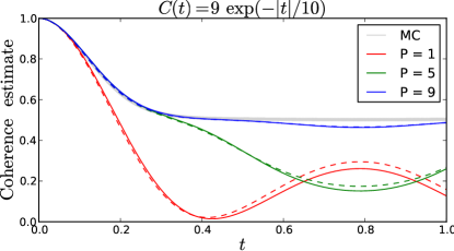
Figure 2: (Color online) A comparison of the predicted time-dependent coherence, $\left\langle{\sigma_{x}(t)}\right\rangle$, for the Hamiltonian given in Eq. (12), with correlation function $C(t)=9\exp(-\left|t\right|/10)$. Solid, colored lines correspond to a stochastic dimension $S=1$, while dashed lines correspond to $S=3$. Grey line is the Monte Carlo result drawn with width equal to the standard error in the estimate. Because of the long correlation time, only one eigenvalue of the KLE is dominant, so it is more efficient to keep the stochastic dimension small and increase the PCE order.

We consider explicitly the stochastic dynamics of a driven quantum two-level system, or qubit, coupled to a classically fluctuating dephasing process:

$$H(t)=\sigma_{x}+\Omega(t)\sigma_{z},$$ (12)

where $\sigma_{x}$ and $\sigma_{z}$ are Pauli matrices. Such a model describes, for example, Rabi oscillations in the presence of dephasing noise Gorman12a ; Young12a , and is particularly relevant for NV centers in diamond Hanson08a ; Ladd10a . Other examples of relevant stochastically-driven systems include dephasing noise in trapped ions Biercuk09a ; Uys09a and $1/f$ noise in superconducting qubits Clarke08a . In the absence of the drift term $\sigma_{x}$, the dephasing dynamics are exactly solvable for any stationary Gaussian process, $\Omega$. However, when this term is included, the Hamiltonian does not commute with itself at different times, and the system is no longer analytically integrable. To illustrate our method, we choose the stochastic process, $\Omega$, to be Gaussian Orenstein-Uhlenbeck type Gardiner04a , with correlation function of the form $C(t)=\alpha^{2}\exp(-\left|t\right|/\tau_{c})$; the coupling parameter, $\alpha$, and the correlation time, $\tau_{c}$, will be specified later. We specify the initial state of the system as $|\sigma_{x}^{+}\rangle$, where $\sigma_{x}|\sigma_{x}^{\pm}\rangle=\pm|\sigma_{x}^{\pm}\rangle$, and we compute the time-dependent coherence, $\left\langle{\sigma_{x}(t)}\right\rangle$. By tuning the noise correlation time and the coupling parameter, this model can explore the convergence of our method with respect to PCE order $P$ and stochastic dimension $S$.

To benchmark the performance of our PCE approach, we compare against MC simulations. MC algorithms approach the problem of computing the stochastic average in Eq. (3) by generating a sufficiently large number of statistically consistent realizations of the stochastic process, $\Omega$, evolving the system with each of the realizations, and averaging the final-time density matrices.

As shown in Fig. 2, our PCE method is capable of reproducing the results of MC simulations with high accuracy, significantly faster than MC. For the example chosen, Monte Carlo required approximately 4000 iterations for convergence, while the most accurate PCE results report here ($P=9$ and $S=3$) required the solution of only 220 coupled equations and ran approximately 20 times faster than the MC simulation. Note that because $\tau_{c}/\tau=10$ in our simulation, only one eigenvalue of the KLE is dominant. In this regime, it is more efficient to keep the stochastic dimension small ($S\leq 3$) and increase the PCE order for improved accuracy. As the order increases from $P=1$ to $P=9$, the accuracy of the PCE coherence increases as a function of time, compared to the converged MC result.

IV Discussion

Our PCE method demonstrates the ability to rapidly and accurately propagate stochastic quantum systems. It outperforms MC simulations in computational efficiency, and has the potential to become an important tool in the study of noisy quantum systems. An area in which we expect the PCE to be particularly useful is in the realm of optimal control (OC). The high computational cost of MC simulations severely limits its use in sequential optimal control simulations. However, PCEs can be both accurate and fast, and they may be easily incorporated as part of a surrogate dynamical model in OC simulations. In this work, the PCE has been formulated to propagate a particular state, however, the equation of motion for the complete dynamical map takes a similar form and may also be adapted easily to PCE methods. Implementation of state-to-state and dynamical map OC will appear in forthcoming work.

An interesting comparison can be made between the PCEs as presented here and another expansion based on orthogonal polynomials: Kubo’s hierarchy equations of motion (HEOM) Kubo69a , and their generalization to all diffusive processes, the DHEOM Sarovar12a . Application of the DHEOM/HEOM demands that the noise be diffusive and have exponentially decaying correlation function, and proceeds by diagonalizing the noise generating functional using of orthogonal polynomials Sarovar12a . Interestingly, though the HEOM and PCE approaches each yields a sparsely-coupled hierarchy of differential equations based on expansions in orthogonal polynomials, they perform well in exactly opposite limits: the HEOM method converges quickly for noise with a short correlation time, while the stochastic dimension of our PCE method converges quickly for noise with a long correlation time. For systems coupled to multiple, uncorrelated noise sources, it may be computationally advantageous to apply different methods for each source: HEOM for noise with short correlation times, PCEs for noise with long correlation times.

Additionally, we have assumed a linear coupling between the system and the stochastic process in Eq. (1). While such a coupling is common Joynt10 , nonlinear interactions are possible, which may increase the coupling density of the differential equations in Eq. (8) by modifying the form of the Galerkin projection of Eq. (10). Strongly nonlinear interactions will yield densely coupled systems of equations, which will increase the computational cost of this method.

Despite the obvious utility of our PCE approach for simulating stochastic quantum systems, it does have limitations. Principal among these is the uncontrolled approximation of the stochastic average, so that the error must be estimated by increasing the PCE order and/or the stochastic dimension of the expansion until convergence is seen. Furthermore, as indicated in Eq. (11), the number of equations to be solved grows combinatorially with both the stochastic dimension and the PCE order; when these are large, the method of Galerkin projections becomes computationally infeasibile. Intermediate between MC and the PCE approach presented here is a non-intrusive formulation of the PCE, so called because its implementation requires only a forward solver for the equations of motion, while the intrusive method presented here requires an explicit solver to propagate the coupled equations resulting from the Galerkin projections. Non-intrusive spectral methods approximate the stochastic average of Eq. (3) by performing a KLE, and using sparse quadrature techniques to perform the average. We plan to implement such techniques in the near future.

V Acknowledgements

We gratefully acknowledge enlightening discussions with Constantin Brif, Cosmin Safta, Maher Salloum, and Mohan Sarovar (SNL-CA). This work was supported by the Laboratory Directed Research and Development program at Sandia National Laboratories. Sandia is a multi-program laboratory managed and operated by Sandia Corporation, a wholly owned subsidiary of Lockheed Martin Corporation, for the United States Department of Energy’s National Nuclear Security Administration under contract DE-AC04-94AL85000.

References

- (1) H.-P. Breuer and F. Petruccione, The theory of open quantum systems (Oxford University Press, Oxford, UK, 2002)
- (2) R. Hanson, V. V. Dobrovitski, A. E. Feiguin, O. Gywat, and D. D. Awschalom, Science 320, 352 (Apr 2008)
- (3) T. D. Ladd, F. Jelezko, R. Laflamme, Y. Nakamura, C. Monroe, and J. L. O’Brien, Nature 464, 45 (Mar 2010)
- (4) W. H. Press, B. P. Flannery, S. A. Teukolsky, and W. T. Vetterling, Numerical Recipes: The Art of Scientific Computing, 2nd ed. (Cambridge University Press, Cambridge, 1992)
- (5) M. Grace, C. Brif, H. Rabitz, I. A. Walmsley, R. L. Kosut, and D. A. Lidar, J. Phys. B: At. Mol. Opt. Phys. 40, S103 (May 2007), Special Issue on the Dynamical Control of Entanglement and Decoherence
- (6) M. D. Grace, C. Brif, H. Rabitz, D. A. Lidar, I. A. Walmsley, and R. L. Kosut, J. Mod. Opt. 54, 2339 (Nov 2007), Special Issue: 37th Winter Colloquium on the Physics of Quantum Electronics, 2-6 January 2007
- (7) D. J. Gorman, K. C. Young, and K. B. Whaley, Phys. Rev. A 86, 012317 (Jul 2012)
- (8) B. J. Debusschere, H. N. Najm, P. P. Peébay, O. M. Knio, R. G. Ghanem, and O. P. Le Maître, J. Sci. Comp. 26, 698 (2004)
- (9) O. P. Le Maître and O. M. Knio, Spectral methods for uncertainty quantification with applications to computational fluid dynamics, Scientific Computation (Springer-Verlag, Berlin, 2010)
- (10) B. D. Ripley, Stochastic Simulation (John Wiley & Sons, Inc., New York, NY, 2008)
- (11) C. W. Gardiner, Stochastic methods: A Handbook for the Natural and Social Sciences, 3rd ed. (Springer-Verlag, Berlin, 2004)
- (12) M. Reed and B. Simon, Methods of Modern Mathematical Physics, Vol. 1 Functional Analysis (Academic Press Ltd., New York, NY, 1980)
- (13) J. J. Sakurai, Modern Quantum Mechanics (Addison-Wesley Publishing Company, Inc., 1994)
- (14) K. C. Young and K. B. Whaley, Phys. Rev. A 86, 012314 (Jul 2012)
- (15) M. J. Biercuk, H. Uys, A. P. VanDevender, N. Shiga, W. M. Itano, and J. J. Bollinger, Nature 458, 996 (April 2009)
- (16) H. Uys, M. J. Biercuk, and J. J. Bollinger, Phys. Rev. Lett. 103, 040501 (Jul 2009)
- (17) J. Clarke and F. K. Wilhelm, Nature 453, 1031 (June 2008)
- (18) C. W. Gardiner and P. Zoller, Quantum Noise: A Handbook of Markovian and Non-Markovian Quantum Stochastic Methods with Applications to Quantum Optics, 3rd ed. (Springer-Verlag, Berlin, 2004)
- (19) R. Kubo, Adv. Chem. Phys. 15, 101 (1969)
- (20) M. Sarovar and M. D. Grace, Phys. Rev. Lett. 109, 130401 (Sep 2012)
- (21) D. Zhou, A. Lang, and R. Joynt, Q. Inf. Proc. 9, 727 (2010), and references therein