Anomalous fluctuations of currents in Sinai-type random chains with strongly correlated disorder

Abstract

We study properties of a random walk in a generalized Sinai model (SM), in which a quenched random potential is a trajectory of a fractional Brownian motion with arbitrary Hurst parameter $H$, $0<H<1$, so that the random force field displays strong spatial correlations. In this case, the disorder-average mean-square displacement (MSD) grows in proportion to $\log^{2/H}(n)$, $n$ being time. We prove that moments of arbitrary order $k$ of the steady-state current $J_{L}$ through a finite segment of length $L$ of such a chain decay as $L^{-(1-H)}$, independently of $k$, which suggests that despite a logarithmic confinement the average current is much higher than its Fickian counterpart in homogeneous systems. Our results reveal a paradoxical behavior such that, for fixed $n$ and $L$, the MSD decreases when one varies $H$ from $0$ to $1$, while the average current increases. This counter-intuitive behavior is explained via an analysis of representative realizations of disorder.

Since the pioneering works kesten ; derrida ; sinai , random walks (RWs) in random media attracted a considerable attention. In part, due to a general interest in dynamics in disordered systems, but also because such RWs found many physical applications, including dynamics of the helix/coil phases boundary in a random heteropolymer pgg ; redner , a random-field Ising model bruinsma ; nattermann , dislocations in disordered crystals harth , mechanical unzipping of DNA walter , translocation of biomolecules through nanopores 9 and molecular motors 10 . Some functionals arising here, e.g., probability currents in finite samples, show up in mathematical finance alain ; greg . Other examples can be found in comtet ; hughes ; sheinman .

In the discrete formulation, a RW evolves in a discrete time on a lattice. At each time step the walker jumps from site $X$ to either site $X+1$ with the site-dependent probability $p_{X}=\frac{1}{2}(1+\varepsilon\cdot s_{X})$, or to the site $X-1$ with the probability $q_{X}=1-p_{X}$, where the amplitude $0<\varepsilon<1$ measures the strength of the disorder and $s_{X}$ are quenched, independent and identically distributed (i.i.d.) random variables (r.v.). One often assumes binomial r.v., i.e., $s_{X}=\pm 1$ with probabilities $p$ and $1-p$, respectively.

In case of no global bias ($p=1/2$), i.e. for the so-called Sinai model (SM), a remarkable result sinai is that for a given environment $\{p_{X}\}$ the squared displacement

$$X_{n}^{2}\sim m(\{p_{X}\})\,\ln^{4}(n)\,,$$ (1)

as $n\to\infty$ with probability almost $1$, where $m(\{p_{X}\})$ is a function of the environment only note2 . Another intriguing feature of the SM concerns transport properties. It was revealed by analysing the probability current $J_{L}$ through a finite Sinai chain of length $L$, that the disorder-average current decays as $1/\sqrt{L}$ gleb ; gleb1 ; gleb2 ; cecile . Curiously enough, despite a logarithmic confinement (1), the disorder-average current appears to be anomalously high, so that such disordered chains offer on average less resistance with respect to transport of particles than homogeneous chains (all $p_{X}\equiv 1/2$) for which one finds Fick’s law $J_{L}\sim 1/L$. In absence of disorder, deviations from Fick’s law can also be found for Lévy walks dhar_derrida . Full statistics of the current has been recently computed for ASEP model kirone .

It is well-known that a RW in uncorrelated random environment $\{p_{X}\}$ can be considered as a one in presence of a random potential $V_{L}$, which represents itself a RW in space. Indeed, on scales $L$ a RW ”explores” the potential

$$V_{L}=\sum_{X=1}^{L-1}\ln\left(\frac{p_{X}}{q_{X}}\right)=\sigma\sum_{X=0}^{L-1}s_{X}\,,\sigma=\ln\left(\frac{1+\varepsilon}{1-\varepsilon}\right)\,,$$ (2)

which is just a RW trajectory with step length $\sigma$. Standard SM, in which the $s_{X}$’s are uncorrelated is now well understood. On the contrary, there hardly exist analytical results for the case where these r.v. are strongly correlated. Such correlations are important, e.g., for the dynamics of the helix-coil boundary in random heteropolymers, where the chemical units are usually strongly correlated gros3 . They are also currently studied in mathematical finance, improving the standard Black-Sholes-Merton (BSM) model fBm_finance . Any exact result for such situations would thus be welcome.

In this Letter, we study properties of random walks in random environments in which the transition probabilities $\{p_{X}\}$ are strongly correlated so that the potential $V_{L}$ in (2) is a fractional Brownian motion (fBm): $V_{L}$ is Gaussian, with $V_{L=0}=0$ and moments

$$\mathbb{E}\left\{V_{L}\right\}=0\,,\,\,\mathbb{E}\left\{(V_{L}-V_{L^{\prime}})^{2}\right\}=\sigma^{2}|L-L^{\prime}|^{2H}\,,$$ (3)

where $\mathbb{E}\{\ldots\}$ here and henceforth denotes averaging over realizations of $V_{L}$ and $0<H<1$. The case $H=1/2$ corresponds to the original SM. For $H<1/2$ the potential is subdiffusive while for $H>1/2$ it is superdiffusive.

The mean squared displacement $\mathbb{E}\{X_{n}^{2}\}$ in a correlated random environment can be estimated as follows. Assuming Arrhenius’ law for the activated dynamics comtet , the time $n_{L}$ required for a particle to diffuse in a disordered potential $V_{L}$ over a scale $L$, is of order $n_{L}\sim e^{V_{L}^{*}}$, where $V_{L}^{*}$ is a typical energy barrier. For $V_{L}$ in (3), $V_{L}^{*}\sim\sigma L^{H}$, so that for sufficiently large times $n$

$$\mathbb{E}\left\{X_{n}^{2}\right\}\sim\sigma^{-2/H}\ln^{2/H}(n)\,.$$ (4)

Our focal interest here is in understanding the behavior of the disorder-average current $J_{L}$ through a finite sample (of length $L$) of such a disordered chain, of its moments of arbitrary order, and eventually, of the full probability density function (pdf) of $J_{L}$. We proceed to show that, while its typical value is exponentially small $J_{{\rm typ}}\sim\exp{(-L^{H})}$, all its moments decay algebraically

$$\mu_{k}(L)\equiv\mathbb{E}\left\{\left({J_{L}}\right)^{k}\right\}\sim A_{k}{L}^{-\theta}\;,\;L\gg 1\,,$$ (5)

where $\theta=1-H$ is the persistence exponent of the fBm krug ; molchan . Recall that the persistence exponent associated to a stochastic process characterizes the algebraic decay of its survival probability $S(n)\sim n^{-\theta}$ majumdar ; aurzada_simon . The $L$-independent constants $A_{k}$ depend in general, on the microscopic details (as the lattice discretization).

The result in (5) is rather astonishing: a) it states that $\mu_{k}(L)$ for arbitrary order $k$ decay in the same way. b) for arbitrary $H$, $0<H<1$, the disorder-average current in such random chains is larger than the Fickian current in homogeneous systems and c) on comparing (4) and (5) for fixed $n$ and $L$ sufficiently large, and varying $H$, one concludes that $\mathbb{E}\{X_{n}^{2}\}$ increases when $H$ goes from $1$ to $0$, while the disorder-average current decreases, which is an absolutely counter-intuitive and surprising behavior.

In what follows we prove (5) and explain this astonishing behavior using three complementary approaches: (i) a rigorous one, based on exact bounds, for the discrete RW in a fBm potential, (ii) scaling arguments for the continuous-space and -time version, which also allows to study the whole pdf of $J_{L}$ and (iii) via numerical simulations. We argue that (5) holds for any potential $V_{L}$, which is the trajectory of a stochastic process with persistence exponent $\theta$: as a matter of fact, such a behavior of $\mu_{k}(L)$ is dominated by the configurations of $V_{L}$ which drift to $-\infty$ without re-crossing the origin and occur with a probability $\sim L^{-\theta}$, yielding the $L$-dependence in (5).

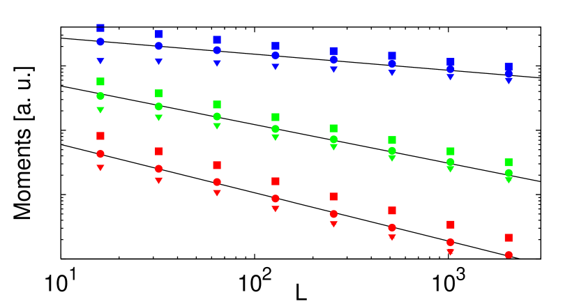
Figure 1: (Color online) $\mathbb{E}\left\{J_{L}\right\}$ (squares) and $\mu_{k}(L)$ with $k=2$ (circles) and $k=3$ (triangles) vs $L$ for the fBm with $H=0.75$, $0.4$ and $0.25$ (from top to bottom). The solid line is $L^{-\theta}$ (5) with $\theta=1-H$. The temperature $T=0.25$ and averaging is performed over $10^{5}$ samples. We use arbitrary units [a.u.] because we vertically shift the data (by a factor $20$ for $H=3/4$, $5$ for $H=0.4$ and $1$ for $H=0.25$). In any case, the prefactors $A_{k}$ are non-universal and model dependent.

Consider first the discrete chain, take a finite segment of length $L$ and impose fixed concentrations of particles at the endpoints, $P_{0}$ and $P_{L}$. For a fixed environment $\{p_{X}\}$, the steady-state current is given by gleb ; gleb1

$$J_{L}=\frac{D_{0}P_{0}}{\tau_{L}}-\frac{D_{0}P_{L}}{\tau^{*}_{L}},$$ (6)

where $D_{0}=1/2$ is the diffusion coefficient of a homogeneous chain, $\tau_{L}$ is the so-called Kesten variable kesten2 :

$$\tau_{L}=1+\frac{p_{1}}{q_{1}}+\frac{p_{1}p_{2}}{q_{1}q_{2}}+\ldots+\frac{p_{1}p_{2}\ldots p_{L-1}}{q_{1}q_{2}\ldots q_{L-1}}\,,$$ (7)

and $\tau_{L}^{*}$ is obtained from (7) by replacements $p_{k}\to q_{L-k}$ and $q_{k}\to p_{L-k}$. Thinking of $L$ as ”time”, one notices that $\tau_{L}$ and $\tau^{*}_{L}$ are time-averaged discretized geometric fractional Brownian motions (they can be thought of as the ”prices” of Asian options within the framework of the fractional BSM model greg ). Note that in absence of a global bias $\mathbb{E}\{1/\tau_{L}\}=\mathbb{E}\{1/\tau^{*}_{L}\}$, and hence, without any loss of generality we set $P_{L}=0$ in what follows. Thus, combining (2, 6, 7) and setting $P_{0}=1$ yields

$$J_{L}=\frac{1}{2}\left(1+\sum_{l=1}^{L-1}\exp\left(V_{l}\right)\right)^{-1}\;.$$ (8)

For typical realizations of $\{p_{X}\}$, the size of $|V_{l}|$ is $\mathcal{O}(l^{H})$ so that the typical current $J_{{\rm typ}}$ is $J_{{\rm typ}}\sim\exp\left(-L^{H}\right)$.

To obtain an upper bound on $\mu_{k}(L)$, consider a given realization of the sequence $V_{1},V_{2},\ldots,V_{L-1}$ and denote the maximal among them as $V_{\max}={\max}_{0\leq i\leq L-1}V_{i}$. From (7) one has $\tau_{L}=(1+\sum_{l=1}^{L-1}V_{l})\geq\exp\left(V_{\max}\right)$, so that $J_{L}^{k}\leq\left({1}/{2}\right)^{k}\exp\left(-kV_{\max}\right)$. Since $\exp\left(-kV_{\max}\right)\to 0$ as $L\to\infty$ (recall that $V_{\max}\sim L^{H}$) the average value of $\exp\left(-kV_{\max}\right)$ is dominated by configurations with $V_{\max}\to 0$. The asymptotic behavior of the pdf $P_{L}(V_{\rm max})$ for fixed $V_{\max}$ and large $L$ is known krug ; molchan , yielding $\ln P_{L}(V_{\max})=\theta\ln L^{-1}+{\cal O}(1)$, where $\theta=1-H$ is the persistence exponent note . Hence, we have

$$\mu_{k}(L)\leq{B_{k}}{L^{H-1}}\,,L\gg 1\,,$$ (9)

where $B_{k}$ is an $L$-independent constant.

To determine a lower bound on $\mu_{k}(L)$ we follow gleb ; gleb1 ; cec and make the following observation: averaging  (8) is to be performed over the entire set $\Omega$ of all possible trajectories $\{V_{l}\}_{1\leq l\leq L}$. Since $\tau_{L}>0$, a lower bound on $\mu_{k}(L)$ can be straightforwardly obtained if one averages instead over some finite subset $\Omega^{\prime}\subset\Omega$ of trajectories with some prescribed properties, that is $\mu_{k}(L)\geq\mathbb{E}_{\Omega^{\prime}}\left\{J_{L}^{k}\right\}$. We choose $\Omega^{\prime}$ as the set comprising all possible trajectories $\{V_{l}\}_{0\leq l\leq L}$ which, starting at the origin at $l=0$, never cross the deterministic curve $Y_{l}=Y_{0}-\alpha\ln(1+l)$ with $Y_{0}>0$ and $\alpha>1$. For any such trajectory $\tau_{L}=1+\sum_{l=1}^{L-1}\exp\left(V_{l}\right)$ is bounded from above by $\sum_{l=0}^{L-1}\exp\left(Y_{l}\right)$, which, in turn, is bounded from above by $\exp(Y_{0})\zeta(\alpha)$, where $\zeta(\alpha)$ is the zeta-function. Hence, we have $\mu_{k}(L)\geq(\exp(Y_{0})\zeta(\alpha)/2)^{-k}\,\mathbb{E}_{\Omega^{\prime}}\left\{1\right\}$, where $\mathbb{E}_{\Omega^{\prime}}\left\{1\right\}$ is, by definition, the survival probability, $S_{L}$ up to time $L$, for a fBm, starting at the origin in presence of a ”moving trap” evolving via $Y_{l}=Y_{0}-\alpha\ln(1+l)$.

For standard Brownian motion ($H=1/2$) in presence of a trap which moves as $-l^{z}$, the leading large-$L$ behavior of the survival probability $S_{L}$ is exactly the same as in the case of an immobile trap, provided that $z<1/2$ krap . It is thus physically plausible to suppose that the same behavior holds for a more general Gaussian process such as a fBm. That is, one expects that for any $H>0$ the leading large-$L$ behavior of $\mathbb{E}_{\Omega^{\prime}}\left\{1\right\}$ will be exactly the same for an immobile trap and for a logarithmically moving trap, i.e., that $S_{L}=\mathbb{E}_{\Omega^{\prime}}\left\{1\right\}\sim Y_{0}^{\theta/H}/L^{\theta}$ as $L\to\infty$ krug ; molchan , where $\theta=1-H$. In fact, this can be shown rigorously aurzada_fbm ; aurz . Consequently, we find

$$\mu_{k}(L)\geq{D_{k}}{L^{H-1}}\;,L\gg 1\,,$$ (10)

where $D_{k}$ is independent of $L$. Note that the bounds in (9) and (10) show the same $L$-dependence and thus yields the exact result announced in (5).

We now turn to a continuous-time and -space dynamics in a disordered fBm potential. The position $x(t)\in[0,L]$ of a particle at time $t$ obeys a Langevin equation : $\dot{x}=-V^{\prime}(x)+\eta(t)$, where $V^{\prime}(x)$ is a quenched random force such that $V(x)$ is a fBm with Hurst exponent $H$ (3) and $\eta(t)$ is a Gaussian thermal noise of zero mean and covariance $\langle\eta(t)\eta(t^{\prime})\rangle=2T\delta(t-t^{\prime})$. The steady-state current and the concentration profile $C(x)$ can be obtained from the corresponding Fokker-Planck equation

$$J_{L}={T}\left({\int_{0}^{L}\,\exp{[{V(x)}/{T}]}\,dx}\right)^{-1}\;,$$ (11)

$$C(x)=\frac{J_{L}}{T}\int_{x}^{L}dx^{\prime}\,\exp{[(V(x^{\prime})-V(x))/T]}\;,$$

[see (6, 8) with $D_{0}=T$ and $P_{0}=1$] remark . The total number of particles is then $N_{L}=\int_{0}^{L}C(x)\,dx$. We focus next on the moments and on the pdf of $J_{L}$ (11).

Instead of $J_{L}/T$, which can be viewed as the inverse of the SM partition function, we study the pdf $\Pi_{T=0}(F)$ of the free energy $F=T\log(J_{L}/T)$. Consider first $T\equiv 0$, in which case $F=E_{\min}=\min_{0\leq x\leq L}V(x)$. Recalling that $V(0)=0$ ($E_{\min}<0$), the cumulative distribution $q_{L}(E)={\Pr}(E_{\min}>-E)$, (with $E>0$), coincides with the probability that up to ’time’ $L$, $V(x)$ starting at $E$ at $x=0$ ’survives’ in presence of an absorbing boundary at $V=0$. For self-affine process, $q_{L}(E)$ takes the scaling form $q_{L}(E)=Q(E/L^{H})$: for $L\gg E^{1/H}$, $q_{L}(E)$ behaves algebraically majumdar , $q_{L}(E)\sim{E^{\theta/H}}/{L^{\theta}}$ ($\theta=1-H$ for fBm krug ; molchan ), while for $L\ll E^{1/H}$, $q_{L}(E)$ is of order one. Hence, one has for $\Pi_{T=0}(F)=\partial_{E}q_{L}(E)\big{|}_{E=-F}$

$$\Pi_{T=0}(F)=\begin{cases}&0\;,\;F>0\\ &L^{-\theta}|F|^{\theta/H-1}\;,\;-L^{H}\ll F<0\\ &\exp(-F^{2}/2L^{2H})\;,\;F\ll-L^{H}\;.\end{cases}$$ (12)

Lastly, the regime $F\ll-L^{H}$ corresponds to a fraction of paths $V(x)$ that propagate from $E$ to zero in a ’time’ $L$. In general, the tail of this probability coincides with the one of the free propagator, which is Gaussian for fBm. What happens at finite $T$ where $F=E-TS$ is now the balance between the energy $E$ and the entropy $S$ ? One expects a particle to be localized close to the minimum $E_{\min}$, which is of order ${\cal O}(L^{H})$, while the maximum entropy $\sim{\cal O}(\ln L)$. Hence when $L\gg 1$ the main contribution to $F$ comes from $E_{\min}$ so that for a given sample at finite $T$, $F$ will be very close to $E_{\min}$. This is corroborated by numerical simulations (see Fig. 2).

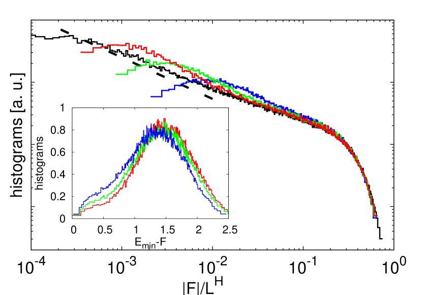
Figure 2: (Color online) Pdf of the free energy $-F/L^{H}$ for different system sizes: $L=64\,(\rm blue),256\,(\rm green),1024\,(\rm red)$. The black curve represents the distribution of $E_{\rm min}/L^{H}$ for $L=4096$. Inset: Pdf of $E_{\min}-F$ for different system sizes: $L=64\,(\rm blue),256\,(\rm green),1024\,(\rm red)$. Histograms are computed using $10^{5}$ samples and setting $T=1$ and $H=3/4$. The dashed line corresponds to $(|F|/L^{H})^{-2/3}$ (12).

We now come back to the current distribution. Very small currents, $J_{L}\ll J_{\rm typ}\sim\exp(-L^{H})$, correspond to $F\ll-L^{H}$ in (12) and one obtains that $P(J_{L})$ is log-normal, $\ln P(J_{L})\propto{-{\ln^{2}(J_{L}/T)}}$. Within the opposite limit, $J_{L}\gg J_{\rm typ}$, one finds from (12) that

$$P(J_{L})\sim\frac{[\log(J_{L}/T)]^{\theta/H-1}}{J_{L}L^{\theta}}\;.$$ (13)

This power-law behavior holds up to a large cut-off value $J_{\max}$. At $T=0$ we have a sharp cut-off at $J_{\max}=1$ (12), while at a finite $T$, $P(J_{L})$ has a fast decay which depends on the fluctuations of $V(x)$ at a short length scale close to the origin $x=0$. For $L\gg 1$, $\mu_{k}(L)$ are dominated by the regime where $J_{\rm typ}\ll J_{L}<J_{\max}\sim{\cal O}(1)$ (13), such that one gets $\mu_{k}(L)\sim 1/{L^{\theta}}$ (5). This calculation shows that (rare) negative persistent potential leads to very large currents. We observe that these rare persistent profiles also exhibit large barriers, growing like $L^{H}$. These barriers stop the particle diffusion and are responsible for the subdiffusive behavior of the mean square displacement. One could expect that these barriers should also affect the behavior of the current. However, by looking at the steady state concentration profile $C(x)$ (11), one can see that large barriers induce a very large number of particles in the system located in the deep valleys of the potential $V(x)$, which allows to sustain a large current.

In our numerical simulations we consider a discrete random potential $V_{k}$, $k=0,1,\ldots L-1$, with $\sigma^{2}=1$, which displays fBm correlations (3). We use a powerful algorithm rosso_fbm ; GRS10 , which allows to generate very long samples of fBm paths. For each sample, we compute the current, $J_{L}=T[\sum_{k=0}^{L-1}\exp(-V_{k}/T)]^{-1}$, the free energy $F=T\ln(J_{L}/T)$ and the ground state energy $E_{\min}=\min_{k}V_{k}$. In Fig. 1 we plot the first three moments as a function of $L$ for different values of $H$. These plots show a very good agreement with our analytical predictions in (5). In Fig. 2, we show that the pdf of the rescaled free energy, $F/L^{H}$, at finite temperature $T$ converges to the pdf of the rescaled ground state energy $E_{\min}/L^{H}$. The reason for this is that, for each sample, the difference between $F$ and $E_{\min}$ grows very slowly with $L$, probably logarithmically (inset of Fig. 2). In the rescaled variables, this difference vanishes when $L\to\infty$.

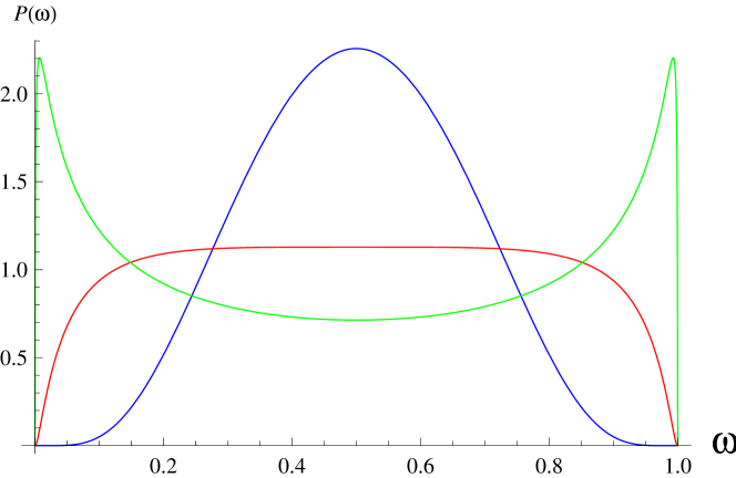
Figure 3: (Color online) The pdf in Eq. (14) for $\sigma^{2}L^{2H}=1/2$ (blue), $\sigma^{2}L^{2H}=2$ (red) and $\sigma^{2}L^{2H}=5$ (green).

We close with an observation that such chains show a transition to a diode-like behavior, when $\xi=\sigma^{2}L^{2H}$ exceeds some critical value $\xi_{c}$. Consider a chain in which at site $X=0$ we maintain a fixed concentration $P_{0}=1$ of, say, ”white” particles and place a sink for them at $X=L$. At $X=L$ we introduce a source which maintains concentration $1$ of ”black” particles, and place a sink for them at site $X=0$. The particles are mutually noninteracting. For a fixed $\{p_{X}\}$ we have counter-currents of white ($J_{L}^{w}$) and black ($J_{L}^{b}$) particles, which obviously obey, on average, $\mathbb{E}\left\{(J_{L}^{w})^{k}\right\}\equiv\mathbb{E}\left\{(J_{L}^{b})^{k}\right\}$ for any $k>0$.

Consider next the random variable: $\omega={J_{L}^{w}}/{(J_{L}^{w}+J_{L}^{b})}={\tau_{L}^{*}}/{(\tau_{L}^{*}+\tau_{L})}$, which probes the likelihood of an event that for a fixed $\{p_{X}\}$ one has $J_{L}^{w}=J_{L}^{b}$. The pdf of $\omega$ can be calculated exactly to give

$$P(\omega)=\frac{1}{\sqrt{2\pi}\omega(1-\omega)\sigma L^{H}}\exp\left(-\frac{\ln^{2}\left(\frac{1-\omega}{\omega}\right)}{2\sigma^{2}L^{2H}}\right)\,.$$ (14)

Remarkably, $P(\omega)$ in (14) changes the modality when $\xi$, (which defines the value of a typical barrier), exceeds a critical value $\xi_{c}=2$ (see Fig. 3). For short chains (or small $\sigma$) $P(\omega)$ is unimodal and centered at $\omega=1/2$: any given sample is transmitting particles in both directions equally well and, most probably, $J_{L}^{w}=J_{L}^{b}$. For $\xi=\xi_{c}$ the pdf is nearly uniform (except for narrow regions at the edges) so that any relation between $J_{L}^{w}$ and $J_{L}^{b}$ is equally probable. Finally, for $\xi>\xi_{c}$ (sufficiently strong disorder and/or a long chain) the symmetry is broken and $P(\omega)$ becomes bimodal with a local minimum at $\omega=1/2$ and two maxima close to $0$ and $1$. This means that a given sample is most likely permeable only in one direction.

- (1) H. Kesten, M. V. Kozlov and F. Spitzer, Compos. Math. 30, 145 (1975).
- (2) B. Derrida and Y. Pomeau, Phys. Rev. Lett. 48, 627 (1982).
- (3) Ya. G. Sinai, Theor. Probab. Appl. 27 256, (1982).
- (4) P. G. de Gennes, J. Stat. Phys. 12, 463 (1975).
- (5) G. Oshanin and S. Redner, EPL 85, 10008 (2009).
- (6) R. Bruinsma and G. Aeppli, Phys. Rev. Lett. 52, 1547 (1984).
- (7) T. Nattermann and J. Vilain, Phase Transit. 11, 5 (1988).
- (8) J. P. Harth and J. Lothe, The theory of dislocations (New York, McGraw-Hill, 1968).
- (9) J.-C. Walter, A. Ferrantini, E. Carlon and C. Vanderzande, Phys. Rev. E 85, 031120 (2012).
- (10) J. Mathe et al., Biophys. J. 87, 3205 (2004).
- (11) Y. Kafri, D. K. Lubensky and D. R. Nelson, Biophys. J. 86, 3373 (2004).
- (12) A. Comtet, C. Monthus and M. Yor, J. Appl. Prob. 35, 255 (1998).
- (13) G. Oshanin and G. Schehr, Quant. Finance 12, 1325 (2012).
- (14) J.-P. Bouchaud, A. Comtet, A. Georges, and P. Le Doussal, Ann. Phys. 201, 285 (1990).
- (15) B. D. Hughes, Random walks and random environments Vol.2 (Clarendon Press, Oxford, 1995).
- (16) M. Sheinman, O. Bénichou, R. Voituriez and Y. Kafri, J. Stat. Mech. P09005 (2010).
- (17) the probability being taken over all random walks of steps, starting at the same point.
- (18) S. F. Burlatsky, G. Oshanin, A. Mogutov and M. Moreau, Phys. Rev. A 45, R6955 (1992).
- (19) G. Oshanin, S. F. Burlatsky, M. Moreau and B. Gaveau, Chem. Phys. 177, 803 (1993).
- (20) G. Oshanin, A. Mogutov and M. Moreau, J. Stat. Phys. 73, 379 (1993).
- (21) C. Monthus and A. Comtet, J. Phys. I France 4, 635 (1994).
- (22) A. Dhar, K. Saito and B. Derrida, preprint arXiv:1207.1184.
- (23) M. Gorissen, A. Lazarescu, K. Mallick, C. Vanderzande, Phys. Rev. Lett. 109, 170601 (2012).
- (24) E. N. Govorun et al., Phys. Rev. E 64, 040903 (2001).
- (25) C. Bender, T. Sottinen and E. Valkeila, in Advanced mathematical methods for finance, (ed. G. Di Nunno and B. Oksendal. Springer, Berlin), pp. 75 (2011), arXiv:1004.3106
- (26) G. M. Molchan, Comm. Math. Phys. 205, 97 (1999).
- (27) J. Krug et al., Phys. Rev. E 56, 2702 (1997).
- (28) S. N. Majumdar, Current Science 77, 370 (1999).
- (29) F. Aurzada and T. Simon, preprint arXiv:1203.6554.
- (30) F. Aurzada, Elect. Comm. in Probab. 16, 392 (2011).
- (31) F. Aurzada and C. Baumgarten, arXiv:1301.0424v1.
- (32) H. Kesten, Acta Math. 131, 207 (1973).
- (33) As a matter of fact, this result can be made more precise by writing the distribution in a scaled form . This implies that actually as .
- (34) C. Monthus, G. Oshanin, A. Comtet, and S. F. Burlatsky, Phys. Rev. E 54, 231 (1996).
- (35) We note that the functional in (11) was studied within a different context in molchan ; MRZ09 , and it was shown that its first moment decreases as with . See also different exact results gleb2 ; cecile for the case.
- (36) S. N. Majumdar, A. Rosso and A. Zoia, Phys. Rev. Lett. 104, 020602 (2010).
- (37) K. Uchiyama, Z. Wahrsch. Verw. Gebiete 54, 75 (1980); P. L. Krapivsky and S. Redner, Am. J. Phys. 64, 546 (1996).
- (38) K. J. Wiese, S. N. Majumdar, A. Rosso, Phys. Rev. E 83, 061141 (2011).
- (39) R. Garcia-Garcia, A. Rosso and G. Schehr, Phys. Rev. E 81, 010102(R) (2010)