Pinned modes in lossy lattices with local gain and nonlinearity

Abstract

We introduce a discrete linear lossy system with an embedded “hot spot” (HS), i.e., a site carrying linear gain and complex cubic nonlinearity. The system can be used to model an array of optical or plasmonic waveguides, where selective excitation of particular cores is possible. Localized modes pinned to the HS are constructed in an implicit analytical form, and their stability is investigated numerically. Stability regions for the modes are obtained in the parameter space of the linear gain and cubic gain/loss. An essential result is that the interaction of the unsaturated cubic gain and self-defocusing nonlinearity can produce stable modes, although they may be destabilized by finite-amplitude perturbations. On the other hand, the interplay of the cubic loss and self-defocusing gives rise to a bistability.

I Introduction

Dissipative spatial solitons, which originate from the interaction of diffraction, self-focusing nonlinearity, and dissipation (gain and loss), have drawn great interest in nonlinear optics Rosanov and, more recently, in plasmonics plasmonics ; Marini . A necessary condition required for the formation of stable solitons is the stability of the zero background. The simplest single-component complex Ginzburg-Landau (CGL) equation with the uniform linear gain is not an appropriate candidate for modeling dissipative solitons, as it violates this condition. Dissipative solitons may be stabilized by a system of linearly coupled CGL equations wg1 that models dual-core waveguides with the linear gain and loss acting in different cores dual ; Pavel ; Chaos ; Marini . Stable solitons can also be generated by the single CGL equations that incorporate the linear loss, cubic gain and quintic loss, which accounts for the nonlinear saturable absorption CQ ; cqgle . In these models, the quintic loss saturates the growth induced by the cubic gain and therefore stabilizes the solitons.

Another method for generating stable localized modes, which has recently drawn considerable attention, relies on the action of linear gain at a “hot spot” (HS, i.e., a localized region in a lossy waveguide HSexact ; HS ; Valery or in a dissipative Bragg grating Mak ). Models with several hot spots spotsExact1 ; spots ; spotsExact2 , as well as with similar extended structures Zezyu , have also been studied. HSs can be created by implanting an appropriate distribution of gain-producing dopants into the waveguide Kip , or by illuminating a uniformly-doped waveguide with external pump beam(s) focused at the designated spot(s). Dissipative solitons pinned to HSs can be stabilized via the balance between the local amplification and uniform loss in the waveguide. In particular, solutions for dissipative solitons pinned to narrow HSs approximated by delta-functions have been found analytically HSexact ; spotsExact1 ; spotsExact2 . Other relevant modes, both one- and two-dimensional, including stable vortices supported by the gain applied to a confined area 2D , have been generated in the numerical form HS ; Valery ; spots . Stable dissipative solitons have also been predicted in a system that combines the uniformly-distributed linear gain and nonlinear loss growing towards the periphery faster than $r^{D}$, where $r$ and $D$ represent the distance from the center and spatial dimension, respectively Barcelona .

An interesting ramification of the configurations mentioned above is the possibility to generate stable solitons supported by localized cubic gain, in the absence of the quintic gain saturation. While dissipative solitons cannot be stable without higher-order nonlinear losses in uniform media Kramer ; ml , it was recently demonstrated Valery that stable dissipative solitons may be pinned to an HS carrying the unsaturated cubic gain and embedded into a uniform linear-loss background. This finding suggests ways to design clean nonlinear soliton amplification that avoids concomitant generation of noise, which is also relevant for plasmonics Korea .

The present work explores the generation of stable solitons in discrete waveguiding arrays (lattices) with a localized unsaturated nonlinear gain. In particular, we demonstrate that this is possible in a linear lattice where the nonlinearity, represented by the self-phase modulation and cubic gain, is applied to a single waveguide (the HS). The lattice CGL system is introduced here as a discrete counterpart of the continuous HS models HSexact ; Valery , and can be used to investigate various effects in photonics, cf. Refs. review ; discrCGL ; Eyal . In particular, it may be used for selective excitation of particular core(s) in an arrayed waveguiding system, if it is uniformly doped, but only the selected core is pumped by an external coherent source of light. In addition to allowing the straightforward experimental implementation review , we demonstrate that the present discrete system supports analytical solutions for discrete solitons (similar to those in the discrete linear Schrödinger equation with embedded nonlinear elements embed ), thus providing a natural platform for exploring the soliton dynamics.

The paper is organized as follows. The discrete CGL equation with HS, and its implicit analytical solutions for pinned modes, are introduced in Sec. II. The linear stability analysis of the solitons against small perturbations is presented in Sec. III, and results of numerical computations of the corresponding eigenvalue spectra are reported in Sec. IV. The predictions of the linear-stability analysis are compared to direct simulations of perturbed evolution of the discrete solitons. In particular, stable solitons are found under the unsaturated nonlinear local gain, provided that the localized nonlinearity is self-defocusing, although finite-amplitude perturbations may destabilize these modes. On the other hand, the interplay of the self-defocusing nonlinearity and cubic loss gives rise to bistability of the pinned modes, which is a sufficiently interesting finding too. The paper is concluded by Sec. V.

II The model

The present work is motivated by the complex Ginzburg-Landau (CGL) equation that models the propagation of an electromagnetic field of amplitude $u(x,z)$ in a lossy waveguide with an embedded HS:

$$\frac{\partial u}{\partial z}=\frac{i}{2}\frac{\partial^{2}u}{\partial x^{2}}-\gamma u+\left[\left(\Gamma_{1}+i\Gamma_{2}\right)+\left(iB-E\right)|u|^{2}\right]\delta(x)u\;.$$ (1)

Here $x$ and $z$ are the transverse and longitudinal coordinates, and $\gamma>0$ is the background linear loss. Delta-function $\delta(x)$ approximates the concentration of the linear gain ($\Gamma_{1}>0$), linear potential ($\Gamma_{2}>0$ corresponds to the local attraction), cubic dissipation $E$ (positive and negative for the loss and gain, respectively), and Kerr nonlinearity $B$ (positive and negative for the self-focusing and defocusing) at the HS.

As the model of an array of guiding cores, replacing a single continual waveguide, Eq. (1) is substituted by its discrete version,

$$\frac{\mathrm{d}u_{m}}{\mathrm{d}z}=\frac{i}{2}\left(u_{m-1}-2u_{m}+u_{m+1}\right)-\gamma u_{m}$$

$$+\left[\left(\Gamma_{1}+i\Gamma_{2}\right)+\left(iB-E\right)|u_{m}|^{2}\right]\delta_{m,0}u_{m}\;,$$ (2)

where $m=0$, $\pm 1$, $\pm 2$, … is the discrete coordinate, $\delta_{m,0}$ is the Kronecker’s symbol, and the coefficient of the linear coupling between adjacent cores is scaled to unity. In optics, the discrete equation can be derived  by means of well-known methods Chr ; discrCGL ; review . In the application to arrays of plasmonic waveguides, which can be built, for example, as a set of metallic nanowires mounted on top of a dielectric structure plasmon-array , this equation can be derived in the adiabatic approximation, when the exciton field may be eliminated in favor of the photonic component (otherwise, the discrete system will be two-component). It is also relevant to mention that the well-known staggering transformation review , $u_{m}(t)\equiv\left(-1\right)^{m}e^{-2it}\tilde{u}_{m}^{\ast}$, where the asterisk stands for the complex conjugate, simultaneously reverses the signs of $\Gamma_{2}$ and $B$, thus rendering the self-focusing and defocusing nonlinearities mutually convertible in the discrete system. In particular, the latter feature is essential for modeling arrays of plasmonic waveguides, where the intrinsic excitonic nonlinearity is self-repulsive. In what follows, we fix the signs of $\Gamma_{2}$ and $B$ by defining $\Gamma_{2}>0$, while $B$ may be positive (self-focusing), negative (self-defocusing), or zero.

As mentioned above, the underlying array can be actually manufactured as a uniform one, with all the cores doped by an appropriate amplifying material, while the HS is singled out by focusing an external pump to a single core. The latter setting is interesting for potential applications, as the location of the HS is switchable.

The model based on Eq. (2) is the subject of the present paper. The Kerr-nonlinearity coefficient, if present, may be normalized to $B=+1$ (self-focusing) or $B=-1$ (self-defocusing). These two cases are considered separately in Sec. IV, along with the case of $B=0$, when the nonlinearity is represented solely by the cubic dissipation localized at the HS.

Dissipative solitons in uniform discrete CGL equations were studied by means of numerical methods in Refs. discrCGL ; Eyal . We seek analytical solutions for stationary modes with real propagation constant $k$ as

$$u_{m}=U_{m}e^{ikz}.$$ (3)

Outside of the HS site, $m=0$, the linear lattice gives rise to the exact solution with real amplitude $A$,

$$U_{m}=A\exp(-\lambda|m|),\;|m|~{}\geq 1,$$ (4)

and complex $\lambda\equiv\lambda_{1}+i\lambda_{2}$, localized modes corresponding to $\lambda_{1}>0$.

The amplitude at the HS (central) site may be different from $A$, and hence we assume

$$U_{0}=A_{R}+iA_{I},$$ (5)

for some real constants $A_{R}$ and $A_{I}$. Substituting Eqs. (3), (4) and (5) into the discrete CGL (2) yields six nonlinear algebraic equations for $A$, $A_{R}$, $A_{I}$, $\lambda_{1}$, $\lambda_{2}$ and $k$. Straightforward considerations demonstrate that any solution has $A_{R}=A$ and $A_{I}=0$, hence the six equations reduce to four:

$$-1+\cosh\lambda_{1}\cos\lambda_{2} = k,$$

$$-\gamma-\sinh\lambda_{1}\sin\lambda_{2} = 0,$$

$$e^{-\lambda_{1}}\sin\lambda_{2}-\gamma+\Gamma_{1}-EA^{2} = 0,$$

$$e^{-\lambda_{1}}\cos\lambda_{2}-1+\Gamma_{2}+BA^{2} = k.$$ (6)

This system of algebraic equations can be solved numerically by means of the Newton’s method for $A$, $\lambda_{1}$, $\lambda_{2}$, and $k$. For instance, with $\gamma=0.5$, $\Gamma_{1}=0.9$, $\Gamma_{2}=0.8$, $B=-1$, and $E=0$ (these parameters correspond to the self-defocusing local nonlinearity and zero cubic loss), a physically relevant solution is $A=0.597$, $\lambda_{1}=0.63$, $\lambda_{2}=-0.85$, and $k=-0.2$. The top panel of Fig. 1 shows the stable evolution of the corresponding mode, produced by simulating Eq. (2) with the help of the fourth-order Runge-Kutta algorithm, using periodic boundary conditions.

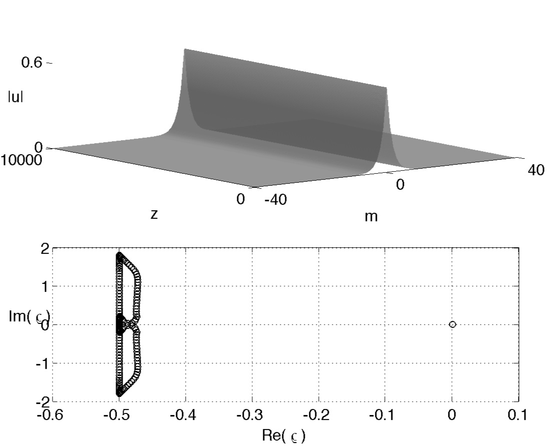
Figure 1: Top: The evolution of the pinned-soliton solution (3) and (4) with $A=0.597$, $\lambda=0.626-0.846i$, and $k=-0.202$. The system’s parameters are $\gamma=0.5$, $\Gamma_{1}=0.9$, $\Gamma_{2}=0.8$, $B=-1$, and $E=0$. Bottom: The spectrum of stability eigenvalues for small perturbations around this solution. All the eigenvalues have non-positive real parts, hence the pinned mode is stable.

Families of pinned modes (3) and their stability are presented in detail below. Linear gain $\Gamma_{1}$ and cubic gain/loss $E$ are used as control parameters in the analysis (in the physical system outlined above, their values may be adjusted by varying the intensity of the external pump). Note that, in the case of $B=E=0$, amplitude $A$ becomes arbitrary and drops out from Eqs. (6), as Eq. (2) becomes linear. In this case, $\Gamma_{1}$ may be considered as another unknown, determined by the balance between the background loss and localized gain in the linear system, which implies the structural instability of the stationary trapped modes in the linear model. In the presence of the nonlinearity, the power balance can be adjusted through the value of the amplitude at given $\Gamma_{1}$, therefore solutions, including stable ones, can be found in a range of values of the linear gain, $\Gamma_{1}$.

III The linear-stability analysis

The stability of the pinned modes was studied by means of the linearization procedure ted . To this end, perturbed solutions were taken as

$$u_{m}=\left[U_{m}+\epsilon V_{m}(z)\right]e^{ikz}\;,$$ (7)

where $V_{m}(z)=X_{m}(z)+iY_{m}(z)$ is a complex perturbation with an infinitesimal amplitude $\epsilon\ll 1$. Substituting this into Eq. (2), one derives the following linear equations:

$$\frac{\mathrm{d}X_{m}}{\mathrm{d}z}=-\frac{1}{2}Y_{m-1}+(k+1)Y_{m}-\frac{1}{2}Y_{m+1}-\gamma X_{m}$$

$$+\delta_{m,0}\left\{\left(\Gamma_{1}X_{m}-\Gamma_{2}Y_{m}\right)\right.$$

$$-B\left[2P_{m}Q_{m}X_{m}+\left(P_{m}^{2}+3Q_{m}^{2}\right)Y_{m}\right]$$

$$\left.-E\left[\left(3P_{m}^{2}+Q_{m}^{2}\right)X_{m}+2P_{m}Q_{m}Y_{m}\right]\right\}\;,$$

$$\frac{\mathrm{d}Y_{m}}{\mathrm{d}z}=\frac{1}{2}X_{m-1}-(k+1)X_{m}+\frac{1}{2}X_{m+1}-\gamma Y_{m}$$

$$+\delta_{m,0}\left\{\left(\Gamma_{2}X_{m}+\Gamma_{1}Y_{m}\right)\right.$$

$$+B\left[\left(3P_{m}^{2}+Q_{m}^{2}\right)X_{m}+2P_{m}Q_{m}Y_{m}\right]$$

$$\left.-E\left[2P_{m}Q_{m}X_{m}+\left(P_{m}^{2}+3Q_{m}^{2}\right)Y_{m}\right]\right\}\;,$$ (8)

where $P_{m}\equiv\mathrm{Re}(U_{m})$ and $Q_{m}\equiv\mathrm{Im}(U_{m})$. An eigenvalue problem is obtained by substituting $X_{m}=\phi_{m}\exp(\rho z)$ and $Y_{m}=\psi_{m}\exp(\rho z)$ into Eqs. (8). The pinned mode is linearly stable provided that all the eigenvalues have $\mathrm{Re}\left(\rho\right)\leq 0$. An example of the stable numerically calculated spectrum for the stationary mode considered in the previous subsection is shown in the bottom panel of Fig. 1.

IV Numerical results

With the help of the methods outlined above, we consider three different cases: (i) the self-defocusing nonlinearity ($B=-1$), (ii) the self-focusing nonlinearity ($B=+1$), and (iii) zero nonlinearity ($B=0$). In each case, the cubic gain ($E<0$) and loss ($E>0$) are investigated separately.

IV.1 The self-defocusing regime ($B=-1$)

The top panel in Fig. 2 shows a typical stable soliton and its eigenvalue spectrum in the self-defocusing regime with the linear and cubic gain applied at the HS, $\Gamma_{1}=0.9048$ and $E=-0.16$ (we stress that the mode is stable in spite of the presence of the unsaturated nonlinear gain). With these parameters, Eqs. (6) yield $A=0.6958$, $\lambda_{1}=0.5615$, $\lambda_{2}=5.2758$, and $k=-0.3795$. When the linear gain is increased from $\Gamma_{1}=0.9048$ to $\Gamma_{1}=0.9936$, the stable solution attains its largest amplitude, $A_{\max}=0.8675$, as shown in the middle panel. With the further increase of the amplitude, an unstable eigenvalue in the spectrum emerges from the origin into the right half-plane. The bottom panel depicts such an unstable solution with amplitude $A=1.074>A_{\max}$, the corresponding linear gain being $\Gamma_{1}=0.7731$.

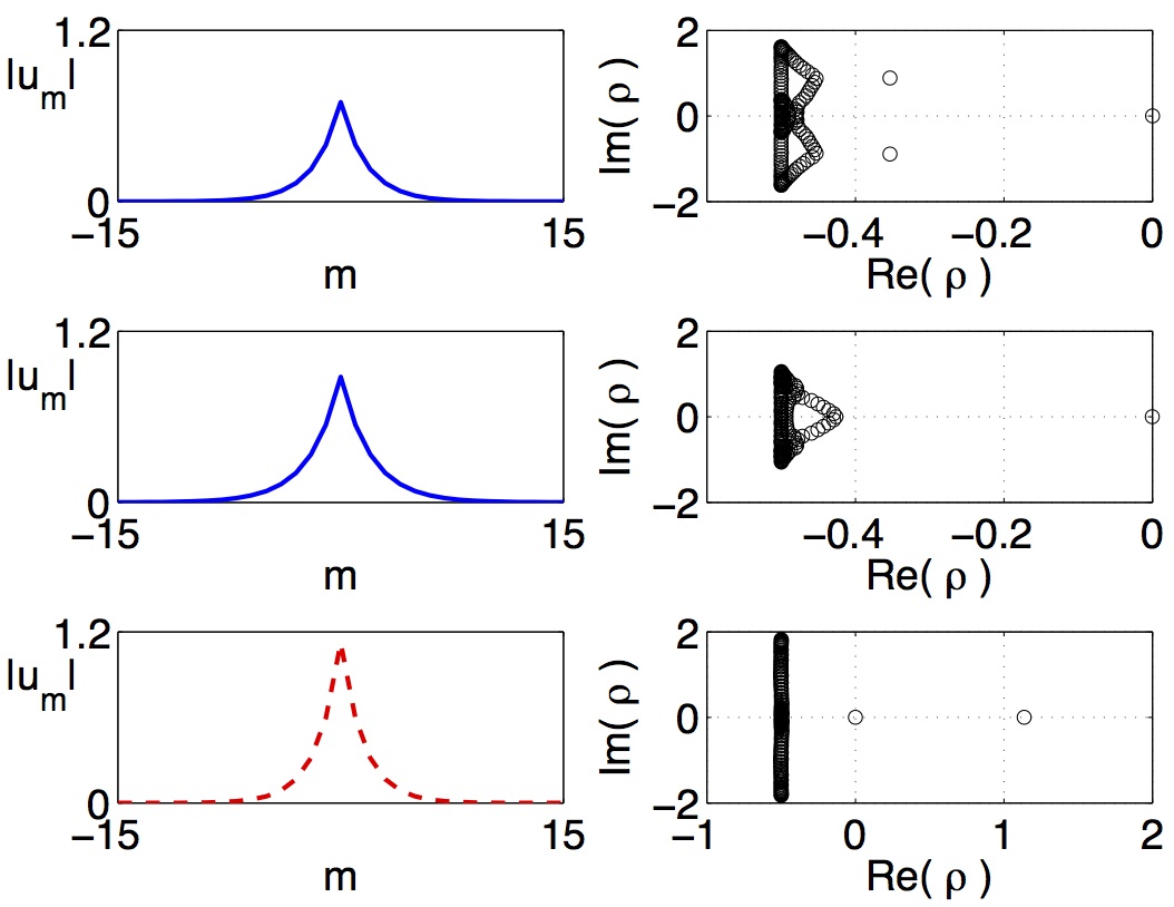
Figure 2: (Color online) Examples of stable and unstable pinned solitons (left) and the corresponding stability spectra (right) in the case of the self-defocusing nonlinearity combined with the cubic unsaturated gain: $B=-1$, $E=-0.016$, $\gamma=0.5$, and $\Gamma_{2}=0.8$. Top: A stable solution found at $\Gamma_{1}=0.9048$. Middle: The stable solution with the largest amplitude, found at $\Gamma_{1}=0.9936$. Bottom: An unstable solution obtained at $\Gamma_{1}=0.7731$ (notice the presence of a positive eigenvalue in the spectrum). Here and in other figures, the blue solid and red dashed lines represent linearly stable and unstable solutions, respectively.

Figure 3 shows amplitude $A$ of the stable (solid) and unstable (dashed) pinned modes as a function of linear gain $\Gamma_{1}>0$ and cubic gain $E<0$. In the absence of the cubic dissipation, i.e., at $E=0$, there exists a stable family of the modes in the region of $0.73\leq\Gamma_{1}\leq 1.11$, with the amplitude ranging from $A=0.08$ to $A=0.89$. Outside this stability region, any solution governed by Eq. (2) either decays to zero, when the linear gain is too small ($\Gamma_{1}<0.73$), or blows up to infinity when it is too large ($\Gamma_{1}>1.11$).

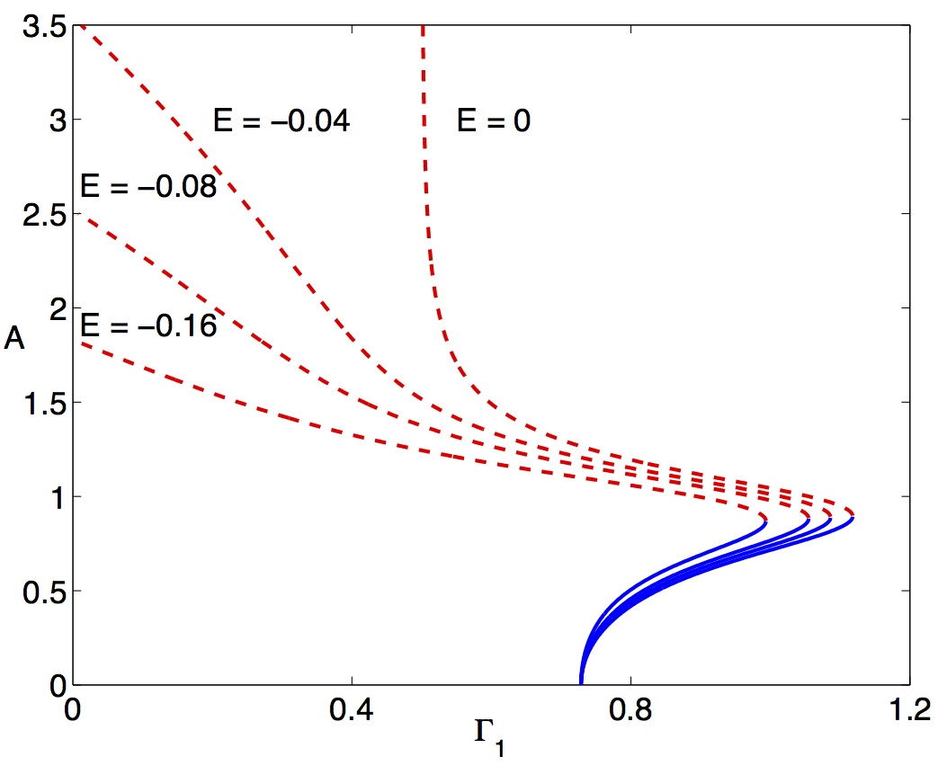
Figure 3: (Color online) Amplitude $A$ of the pinned soliton as a function of linear ($\Gamma_{1}$) and cubic ($E\leq 0$) gain. The other parameters are $\gamma=0.5$, $\Gamma_{2}=0.8$, and $B=-1$.

Figure 3 shows that, when the cubic gain increases, the largest amplitude of the stable soliton and the corresponding linear gain drop, but only by small amounts. Naturally, the bifurcation of the zero solution $A=0$ into the pinned mode takes place at a particular value $\Gamma_{1}=0.7286$, regardless of the value of $E$. On the contrary, the unstable branches show a large variation in amplitude as $E$ varies. At $E=0$, there is a vertical asymptote of the unstable branch exactly at $\Gamma_{1}=0.5$. This implies that, if the local linear gain is too weak, i.e., $\Gamma_{1}<0.5$, it cannot compensate the background loss without the contribution from the nonlinear gain. Although Fig. 3 shows the unstable branches only in the region of $\Gamma_{1}\geq 0$, the curves corresponding to $E<0$ extend to the region of $\Gamma_{1}<0$ (linear loss). These unstable solitons are supported by the nonlinear gain alone.

As mentioned in the Introduction, the existence of the stability region for the pinned modes in the absence of the gain saturation is a remarkable feature of the system. On the other hand, the stability region is (quite naturally) much broader in the case of the cubic loss, $E>0$. Figure 4 shows the respective solution branches obtained with the localized self-defocusing nonlinearity. When the cubic loss is small, e.g., $E=0.01$, there are two distinct families of stable modes, representing broad small-amplitude ($A\leq 0.89$) and narrow large-amplitude ($A\geq 2.11$) ones. These two stable families are linked by an unstable branch with the amplitudes in the interval of $0.89<A<2.11$. There is a range of values of the linear gain, $0.73\leq\Gamma_{1}\leq 1.13$, for which the two stable branches coexist, thus making the system bistable. Figure 5 shows the coexisting stable solutions in the bistability region. In direct simulations, a localized input evolves into either of these two stable solutions, depending on the initial amplitude. With the increase of $E$, the amplitude drops to compensate the growing nonlinear loss, stretching the solution curves in Fig. 4 in the horizontal direction. Simultaneously, the bistability region and the unstable branch shrink. Eventually, both of them disappear at $E\approx 0.66$.

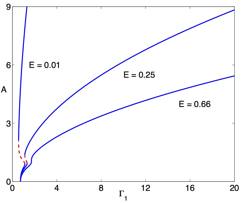
Figure 4: (Color online) Solution branches in the case of the cubic loss ($E>0$). The other parameters are same as those in Fig. 3.

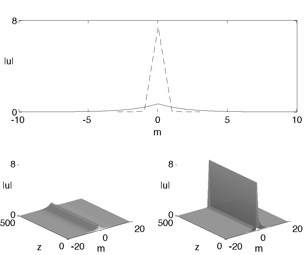
Figure 5: The coexistence of stable small- and large-amplitude pinned modes (top), and the corresponding evolution of perturbed solutions (bottom) at $E=0.01$, in the bistability region. Inputs with amplitudes $A=0.3$ and $A=2$ evolve into the small-amplitude and large-amplitude stationary modes, respectively. The other parameters are $\gamma=0.5$, $\Gamma_{1}=1$, $\Gamma_{2}=0.8$, and $B=-1$.

IV.2 The self-focusing regime ($B=+1$)

For the self-focusing nonlinearity, $B=+1$, the branches of pinned modes (3) are shown in Fig. 6 as functions of $\Gamma_{1}$ and $E$. Under the action of the self-focusing, all the pinned modes are unstable without the cubic loss, i.e., at $E\leq 0$. The left panel of Fig. 7 demonstrates that this instability quickly leads to a blowup of the dissipative soliton. For the parameters considered here, all the unstable solutions originate from point $\Gamma_{1}=0.73$. There is a vertical asymptote at $\Gamma_{1}=0.5$ for the unstable solutions corresponding to $E=0$. These observations are identical to those made in the case of the self-defocusing nonlinearity ($B=-1$, see Figs. 3 and 4.)

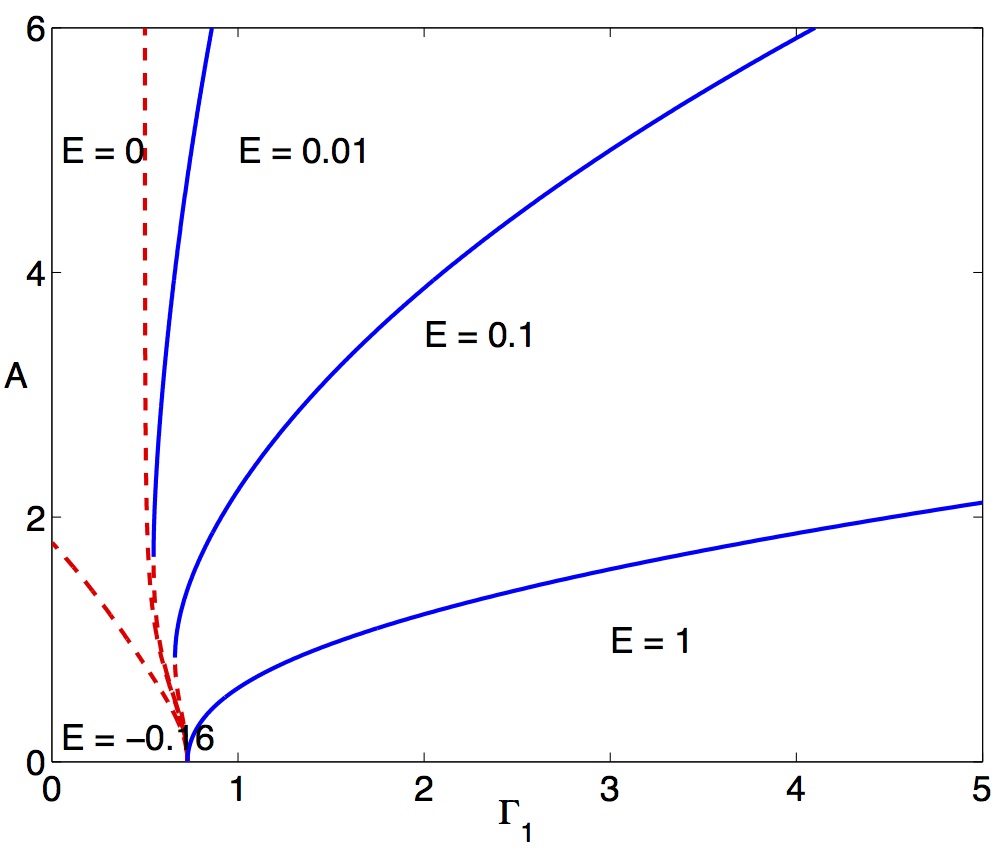
Figure 6: (Color online) Amplitude $A$ of the pinned mode as a function of the linear gain ($\Gamma_{1}$) and cubic loss ($E$) in the model with the self-focusing nonlinearity. The other parameters are $\gamma=0.5$, $\Gamma_{2}=0.8$, and $B=+1$.

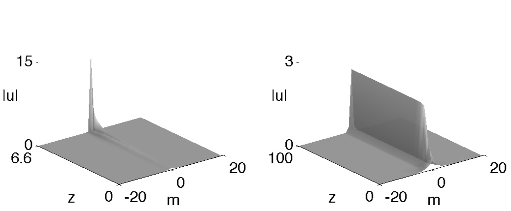
Figure 7: The evolution of perturbed solitons at $E=-0.1$ (left) and $E=0.1$ (right). The other parameters are $\gamma=0.5$, $\Gamma_{1}$, $\Gamma_{2}=0.8$, and $B=1$.

As shown in the right panel of Fig. 7, the dynamical blowup is naturally prevented by the cubic loss ($E>0$). Figure 6 shows the solution branches for this case too. When linear gain $\Gamma_{1}$ falls below a certain threshold, the modes do not exist, as the background loss cannot be compensated. In this case, all initial condition decay to zero. Once $\Gamma_{1}$ exceeds the threshold, the system supports the localized modes, which remain stable even at very large values of $\Gamma_{1}$. Figure 8 shows some representative examples. For instance, with linear gain $\Gamma_{1}=0.9991$, the system supports a stable pinned mode of amplitude $A=2.217$ (the top panel). The stable solution with the smallest amplitude ($A=0.8521$) is found at $\Gamma_{1}=0.6616$ (the middle panel). The solutions with amplitudes $A<0.8521$ are unstable—for instance, the one shown in the bottom panel of Fig. 8

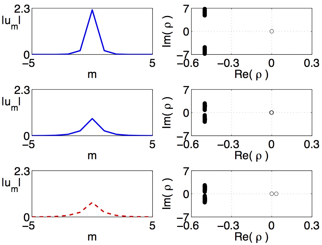
Figure 8: (Color online) Examples of stable and unstable pinned solitons (left) and the corresponding stability spectra (right) in the case of the self-focusing nonlinearity combined with the cubic loss: $B=1$, $E=0.1$, $\gamma=0.5$, and $\Gamma_{2}=0.8$. Top and middle: Stable solutions found at $\Gamma_{1}=0.9991$ and $\Gamma_{1}=0.6616$, respectively. Bottom: An unstable solution obtained at $\Gamma_{1}=0.6648$. In the latter case, there is a positive eigenvalue at $\rho=0.034$.

IV.3 Zero Kerr Nonlinearity ($B=0$)

We have also studied the pinned modes in the case of $B=0$, when the nonlinearity at the HS is represented solely by the cubic gain or loss, $E\neq 0$. Figure 9 shows the respective solution branches corresponding to different values of $E$. The linear stability analysis shows that all these solutions are unstable in the presence of the cubic gain ($E<0$), while the solutions corresponding to the nonlinear loss, $E>0$, are always stable. An interesting feature found here is that the stable and unstable branches in the parameter space are symmetric about the solution for $E=0$. This particular branch has an arbitrary amplitude, as there is no nonlinearity when both $B$ and $E$ vanish. All the solutions belonging to this branch correspond to linear gain $\Gamma_{1}=0.73$, which is again the critical value at which the zero background bifurcates into the pinned mode (see Figs. 3, 4 and 6). Several stable and unstable modes and their linear spectra are shown for the case of $B=0$ and different values of $E$ in Fig. 10.

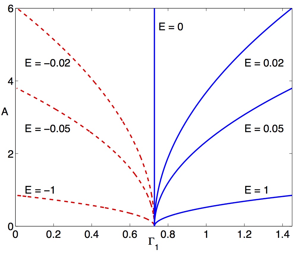
Figure 9: (Color online) Solution branches as a function of the cubic gain or loss $E$ in the case of $B=0$. The other parameters are the same as those in Fig. 7.

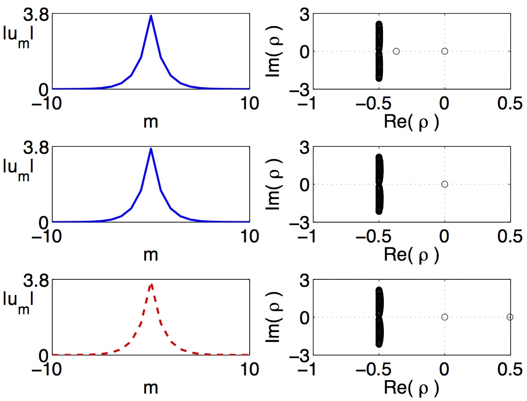
Figure 10: (Color online) Examples of stable and unstable pinned modes (left) and the corresponding stability spectra (right) in the absence of the Kerr nonlinearity ($B=0$). All these solutions have the same amplitudes, $A=3.687$. The other parameters are $\gamma=0.5$, and $\Gamma_{2}=0.8$. Top: A stable solution found at $E=0.02$ with $\Gamma_{1}=1.0004$. Middle: A stable solution found in the linear system, with $E=0$ and $\Gamma_{1}=0.73$ (the amplitude is arbitrary in this case). Bottom: An unstable solution obtained at $E=-0.02$ with $\Gamma_{1}=0.4568$. In the latter case, there is a positive eigenvalue, $\rho=0.4955$.

IV.4 Stability and instability of the pinned modes with respect to finite perturbations

It has been shown above that, while the pinned modes may be stable against infinitesimal perturbations under the combined action of the self-defocusing nonlinearity ($B=-1$) and unsaturated nonlinear gain ($E\leq 0$), the respective stability area is much smaller than that in the case of the nonlinear loss ($E>0$), see Figs. 3 and 4. The apparent fragility of the dissipative solitons in the case of $E\leq 0$, and their robustness at $E>0$ suggest an investigation to check the stability of these two types of the pinned modes against finite-amplitude perturbations, which we have carried out by means of systematic simulations of the evolution of the modes perturbed by reasonably large initial disturbances where linearization will not be an adequate approximation initial disturbances. The conclusion is that the “robust” solitons, found at $E>0$, are completely stable against arbitrary, finite amplitude perturbations. On the other hand, one can always destroy the “fragile” modes, which are stable against infinitesimal perturbations at $E\leq 0$, by applying perturbations of a sufficiently large amplitude. If, in particular, the finite disturbance is applied by suddenly making its amplitude larger than it is in the stationary solution (“stretching”), the soliton will blow up if the stretching factor exceeds a particular critical value. The corresponding instability borders for the solitons with $E=-0.2$ and $E=0$ are displayed in Fig. 11.

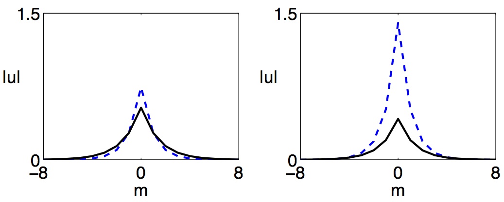
Figure 11: (Color online) The blue dashed curves show the largest initial disturbance, corresponding to the sudden “stretch” of the soliton, after the application of which the pinned dissipative soliton still relaxes back into the original form. A yet stronger stretch quickly initiates a blowup. The left and right panels pertain to $E=-0.2$ and $0$, respectively. The other parameters being $B=-1$, and $\Gamma_{1}=\Gamma_{2}=0.8$.

In addition, the blowup of the linearly stable but “fragile” pinned mode, caused by arbitrary finite amplitude perturbations, and, simultaneously, the full stability of the “robust” mode against still stronger perturbations, are illustrated by their evolution histories presented in Fig. 12. It may be concluded that the entire space of the initial conditions is the attraction basin of the latter mode, while for the one supported by the unsaturated cubic gain the attraction basin is quite narrow.

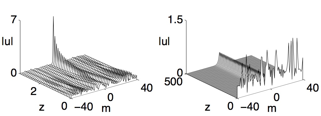
Figure 12: The left panel: The evolution of a strongly perturbed “fragile” pinned mode, at $E=-0.2$. The right panel: the same, but for $E=+0.2$. Other parameters are as in Fig. 11. The other parameters are same as those used in Fig. 11.

V Conclusions

We have introduced the discrete dynamical system based on the linear lossy lattice into which a single nonlinear site with the linear gain (HS, “hot spot”) is embedded. The system can be readily implemented in the form of an array of optical or plasmonic waveguides, admitting selective excitation of individual cores, by the local application of the pump to the uniformly doped cores. Solutions for solitons pinned to the central site were found in the implicit analytical form, and their stability against infinitesimal and finite perturbations was investigated numerically. Stability regions for the solitons have been identified in the parameter plane of the most essential control parameters of the system, viz., the linear gain $\Gamma_{1}$ and cubic dissipation $E$. A nontrivial finding is a (rather small) stability area for the solitons supported by the combination of the local nonlinear unsaturated gain and self-defocusing cubic nonlinearity. On the other hand, the combination of the cubic loss and self-defocusing nonlinearity gives rise to the bistability of the pinned solitons. In the former case, the collapse of the linearly stable soliton is caused by finite amplitude perturbations. These features may be promising for potential applications, and call for an experimental implementation.

The work may be naturally extended in different directions. In particular, it will be interesting to investigate localized modes pinned by pairs of hot spots (cf.the analysis of a discrete counterpart of the continuous model of Ref. spotsExact2 ). A challenging possibility is to develop the analysis for modes pinned to the hot spot embedded into a two-dimensional linear lossy lattice. In that case, an analytical solution is not available even for the linear lattice, hence the entire analysis should be done in a numerical form.

- (1) N. N. Rosanov, Spatial Hysteresis and Optical Patterns (Springer: Berlin, 2002).
- (2) N. Lazarides and G. P. Tsironis, Phys. Rev. E 71, 036614 (2005); Y. M. Liu, G. Bartal, D. A. Genov, and X. Zhang, Phys. Rev. Lett. 99, 153901 (2007); E. Feigenbaum and M. Orenstein, Opt. Lett. 32, 674 (2007); I. R. Gabitov, A. O. Korotkevich, A. I. Maimistov, and J. B. Mcmahon, Appl. Phys. A 89, 277 (2007); A. R. Davoyan, I. V. Shadrivov, and Y. S. Kivshar, Opt. Exp. 17, 21732 (2009); K. Y. Bliokh, Y. P. Bliokh, and A. Ferrando, Phys. Rev. A 79, 041803 (2009); E. V. Kazantseva and A. I. Maimistov, ibid. 79, 033812 (2009); Y.-Y. Lin, R.-K. Lee, and Y. S. Kivshar, Opt. Lett. 34, 2982 (2009); A. Marini and D. V. Skryabin, ibid. 81, 033850 (2010).
- (3) A. Marini, D. V. Skryabin, and B. A. Malomed, Opt. Exp. 19, 6616 (2011).
- (4) J. N. Kutz and B. Sanstede, Optics Express 16, 636; M. O. Williams and J. N. Kutz, ibid. 17, 18320.
- (5) B. A. Malomed and H. G. Winful, Phys. Rev. E 53, 5365 (1996); J. Atai and B. A. Malomed, Phys. Rev. E 54, 4371 (1996); H. Sakaguchi and B. A. Malomed, Physica D 147, 273 (2000).
- (6) P. V. Paulau D. Gomila, P. Colet, N. A. Loiko, N. N. Rosanov, T. Ackemann, and W. J. Firth, Opt. Exp. 18, 8859 (2010).
- (7) B. A. Malomed, Chaos 17, 037117 (2007).
- (8) B. A. Malomed, Physica D 29, 155 (1987); O. Thual and S. Fauve, J. Phys. (France) 49, 1829 (1988); W. van Saarloos and P. Hohenberg, Phys. Rev. Lett. 64, 749 (1990); V. Hakim, P. Jakobsen and Y. Pomeau, Europhys. Lett. 11, 19 (1990); B. A. Malomed and A. A. Nepomnyashchy, Phys. Rev. A 42, 6009 (1990); P. Marcq, H. Chaté, and R. Conte, Physica D 73, 305 (1994); T. Kapitula and B. Sandstede, J. Opt. Soc. Am. B 15, 2757 (1998).
- (9) N. N. Akhmediev, V. V. Afanasjev, J. M. Soto-Crespo, and S. Wabnitz, Phys. Rev. Lett. 79, 4047 (1997); A. Komarov, H. Leblond, and F. Sanchez, Phys. Rev. E 72, 025604 (2005); J. N. Kutz, SIAM Rev. 48, 629 (2006); W. Renninger, A. Chong, and F. Wise, Phys. Rev. A 77, 023814 (2008); E. Ding and J. N. Kutz, J. Opt. Soc. Am. B 26, 2290 (2009).
- (10) C.-K. Lam, B. A. Malomed, K. W. Chow, and P. K. A. Wai, Eur. Phys. J. Special Topics 173, 233 (2009).
- (11) Y. V. Kartashov, V. V. Konotop, and V. A. Vysloukh, EPL 91, 340003 (2010).
- (12) O. V. Borovkova, V. E. Lobanov, and B. A. Malomed, EPL 97, 44003 (2012).
- (13) W. C. K. Mak, B. A. Malomed, and P. L. Chu, Phys. Rev. E 67, 026608 (2003).
- (14) C. H. Tsang, B. A. Malomed, C.-K. Lam, and K. W. Chow, Eur. Phys. J. D 59, 81 (2010)
- (15) D. A. Zezyulin, Y. V. Kartashov, and V. V. Konotop, Opt. Lett. 36, 1200 (2011); Y. V. Kartashov, V. V. Konotop, and V. A. Vysloukh, Phys. Rev. A 83, 041806(R) (2011); D. A. Zezyulin, V. V. Konotop, and G. L. Alfimov, Phys. Rev. E 82, 056213 (2010).
- (16) C. H. Tsang, B. A. Malomed, and K. W. Chow, Phys. Rev. E 84, 066609 (2011).
- (17) D. A. Zezyulin, G. L. Alfimov, and V. V. Konotop, Phys. Rev. A 81, 013606 (2010); F. K. Abdullaev, V. V. Konotop, M. Salerno, and A. V. Yulin, Phys. Rev. E 82, 056606 (2010).
- (18) J. Hukriede, D. Runde, and D. Kip, J. Phys. D: Appl. Phys. 36, R1 (2003).
- (19) V. Skarka, N. B. Aleksić, H. Leblond, B. A. Malomed, and D. Mihalache, Phys. Rev. Lett. 105, 213901 (2010); V. E. Lobanov, Y. V. Kartashov, V. A. Vysloukh, and L. Torner, Opt. Lett. 36, 85 (2011); O. V. Borovkova, V. E. Lobanov, Y. V. Kartashov, and L. Torner, ibid. 36, 1936 (2011); O. V. Borovkova, Y. V. Kartashov, V. E. Lobanov, V. A. Vysloukh, and L. Torner, ibid. 36, 3783 (2011); O. V. Borovkova, V. E. Lobanov, Y. V. Kartashov, and L. Torner, Opt. Lett. 36, 1936 (2011).
- (20) O. V. Borovkova, Y. V. Kartashov, V. A. Vysloukh, V. E. Lobanov, B. A. Malomed, and L. Torner, Opt. Exp. 20, 2657 (2012).
- (21) W. Schöpf and L. Kramer, Phys. Rev. Lett. 66, 2316 (1991).
- (22) T. Kapitula, J. N. Kutz, and B. Sandstede, J. Opt. Soc. Am. B 19, 740 (2002).
- (23) S. Kim, J. H. Jin, Y. J. Kim, I. Y. Park, Y. Kim, and S. W. Kim, Nature 453, 757 (2008).
- (24) F. Lederer, G. I. Stegeman, D. N. Christodoulides, G. Assanto, M. Segev, and Y. Silberberg, Phys. Rep. 436, 1 (2008).
- (25) D. N. Christodoulides and R. I. Joseph, Opt. Lett. 13, 794 (1988).
- (26) A. Christ, S. G. Tikhodeev, N. A. Gippius, J. Kuhl, and H. Giessen, Phys. Rev. Lett. 91, 183901 (2003); A. Christ, T. Zentgraf, J. Kuhl, S. G. Tikhodeev, N. A. Gippius, and H. Giessen, Phys. Rev. B 70, 125113 (2004); Y. S. Bian, Z. Zheng, X. Zhao, Y. L. Su, L. Liu, J. S. Liu, J. S. Zhu, and T. Zhou, IEEE Phot. Tech. Lett. 24, 1279 (2012).
- (27) N. K. Efremidis and D. N. Christodoulides, Phys. Rev. E 67, 026606 (2003); K. Maruno, A. Ankiewicz, and N. Akhmediev, Opt. Commun. 221, 199 (2003); Phys. Lett. A 347, 231 (2005); A. Mohamadou, A. K. Jiotsa, and T. C. Kofane, Phys. Rev. E 72, 036220 (2005); C. Dai and J. Zhang, Opt. Commun. 263, 309 (2006); N. K. Efremidis, D. N. Christodoulides, and K. Hizanidis, Phys. Rev. A 76 , 043839 (2007); N. I. Karachalios, H. E. Nistazakis, and A. N. Yannacopoulos, Discr. Cont. Dyn. Syst. 19, 711 (2007); D. Mihalache, D. Mazilu, and F. Lederer, Eur. Phys. J. Special Topics 173, 255 (2009); C. Mejia-Cortes, J. M. Soto-Crespo, M. I. Molina, and R. A. Vicencio, Phys. Rev. A 82, 063818 (2010); C. Mejia-Cortes, J. M. Soto-Crespo, R. A. Vicencio, and M. I. Molina, ibid. 83, 043837 (2011).
- (28) E. Kenig, B. A. Malomed, M. C. Cross, and R. Lifshitz, Phys. Rev. E 80, 046202 (2009).
- (29) M. I. Molina and G. Tsironis, Phys. Rev. B 47, 15330 (1993); B. C. Gupta and K. Kundu, ibid. 55, 894 (1997); V. A. Brazhnyi and B. A. Malomed, Phys. Rev. A 83, 053844 (2011).
- (30) E. D. Farnum and J. N. Kutz, J. Opt. Soc. Am. B 25, 1002 (2008).