Nuclear shadowing in deep inelastic scattering on nuclei: a closer look

Abstract

The measurement of the nuclear structure function $F_{2}^{A}(x,Q^{2})$ at the future electron-ion collider (EIC) will be of great relevance to understand the origin of the nuclear shadowing and to probe gluon saturation effects. Currently there are several phenomenological models, based on very distinct approaches, which describe the scarce experimental data quite successfully. One of main uncertainties comes from the schemes used to include the effects associated to the multiple scatterings and to unitarize the cross section. In this paper we compare the predictions of three distinct unitarization schemes of the nuclear structure function which use the same theoretical input to describe the projectile-nucleon interaction. In particular, we consider as input the predictions of the Color Glass Condensate formalism, which reproduce the inclusive and diffractive $ep$ HERA data. Our results demonstrate that the experimental analysis of $F_{2}^{A}$ will be able to discriminate between the unitarization schemes.

I Introduction

The measurement of the nuclear structure function in deep inelastic electron-nucleus scattering (DIS) is the best way to improve our knowledge of the nuclear parton distributions and QCD dynamics in the high energy regime (See, e.g.armesto_review ; frank_review ). However, after more than 30 years of experimental and theoretical studies, a standard picture of nuclear modifications of structure functions and parton densities has not yet emerged. Fixed target DIS measurement on nuclei revealed that the ratio of nuclear to nucleon structure functions (normalized by the atomic mass number) is significantly different from unity. In particular, these data demonstrate an intricate behavior, with the ratio being less than one at large $x$ (the EMC effect) and at small $x$ (shadowing) and larger than one for $x\approx 10^{-1}$ (antishadowing). The existing data were taken at lower energies e665 and therefore the perturbative QCD regime ($Q^{2}\geq 1$ GeV²) was explored only for relatively large values of the (Bjorken) $x$ variable ($x>10^{-2}$). Experimentally, this situation will hopefully change with a future high energy electron-ion collider (EIC) (For recent reviews see, e.g. erhic ; lhec ), which is supposed to take data at higher energies and explore the region of small $x$ ($x<10^{-2}$) in the perturbative QCD regime.

The theory of nuclear effects in DIS is still far from being concluded. The straightforward use of nucleon parton distributions evolved with DGLAP equations and corrected with a nuclear modification factor determined by fitting the existing data as in Refs. eks1 ; eks2 ; hkn ; ds ; eps1 ; eps2 is well justified only in the large $Q^{2}$ region and not too small $x$. Moreover, these approaches do not address the fundamental problem of the origin of the nuclear shadowing and cannot be extended to small $x$, where we expect to see new interesting physics related to the non-linear aspects of QCD and gluon saturation (For reviews see Ref. hdqcd ). Currently, there are several phenomenological models which predict different magnitudes for the shadowing in the nuclear structure function based on distinct treatments for the multiple scatterings of the partonic component of the virtual photon, assumed in general to be a quark-antiquark ($q\bar{q}$) color dipole. Some works armesto_glauber ; erike_inclusive ; simone_hq ; erike_exclusive address the origin of the nuclear shadowing through the Glauber-Gribov formalism glauber ; gribov in the totally coherent limit ($l_{c}\approx 1/2m_{N}x\gg R_{A}$, where $l_{c}$ is coherence length), which considers the multiple scattering of the color dipole with a nucleus made of nucleons whose binding energy is neglected. In the high energy limit, the eikonal approximation is assumed, with the dipole keeping a fixed size during the scattering process. In this approach the total photon-nucleus cross section is given by

$$\sigma_{\gamma^{*}A}=\int d^{2}r\,\int dz|\psi(r,z)|^{2}\sigma_{dA}(x,r)$$ (1)

where $|\psi(r,z)|^{2}$ is the probability of the photon to split into a $q\bar{q}$ pair of size $r$ and $\sigma_{dA}(x,r)$ is the dipole-nucleus cross section, which is expressed as armesto_glauber

$$\sigma_{dA}(x,r)=\int d^{2}b\,2\,\left[1-\exp\left(-\frac{1}{2}A\,T_{A}(b)\sigma_{dp}(x,r)\right)\right]$$ (2)

with $T_{A}(b)$ being the nuclear thickness function and $\sigma_{dp}(x,r)$ is the dipole-proton cross section. It must be stressed that once $\sigma_{dp}(x,r)$ is fixed, the extension to the nuclear case is essentially parameter free in this approach. In the Glauber formula (2) it is assumed that the dipole undergoes several elastic scatterings on the target. Although reasonable and phenomenologically successful this assumption deserves further investigation. This model can be derived in the classical approach of the Color Glass Condensate formalism raju_acta .

Another approach largely used in the literature is based on the connection between nuclear shadowing and the cross section for the diffractive dissociation of the projectile capella ; frank_nuc ; armesto_alba ; armesto_dif , which was established long time ago by Gribov gribov . Its result can be derived using reggeon calculus reggeon and the Abramovsky-Gribov-Kancheli (AGK) cutting rules agk and is a manifestation of the unitarity. This formalism can be used to calculate directly cross sections of photon-nucleus scattering for the interaction with two nucleons in terms of the diffractive photon-nucleon cross section. In this formalism, the total photon-nucleus cross section is expressed as a series containing the contribution from multiple scatterings (1, 2, $\dots$):

$$\sigma_{\gamma^{*}A}=\sigma_{\gamma^{*}A}^{(1)}+\sigma_{\gamma^{*}A}^{(2)}+\sigma_{\gamma^{*}A}^{(3)}+\cdots\,$$ (3)

with the first term being the one that arises from independent scattering of the photon off $A$ nucleons:

$$\sigma_{\gamma^{*}A}^{(1)}=A\,\sigma_{\gamma^{*}p}$$ (4)

and the first correction to the non-additivity of cross sections being

$$\sigma_{\gamma^{*}A}^{(2)}=-4\pi A(A-1)\int d^{2}b\ T_{A}^{2}(b)\int_{M^{2}_{\mathrm{min}}}^{M^{2}_{\mathrm{max}}}dM^{2}\left.\frac{d\sigma^{\mathcal{D}}_{\gamma^{*}{\rm p}}}{dM^{2}dt}\right|_{t=0}F_{A}^{2}(t_{\mathrm{min}})$$ (5)

where $M^{2}$ is the mass of the diffractively produced system, $F_{A}$ is the nucleus form factor which takes into account the coherence effects and the differential $\gamma^{*}p$ cross section for diffractive dissociation of the virtual photon appearing in (5) is given by:

$$\left.\frac{d\sigma^{\mathcal{D}}_{\gamma^{*}{\rm p}}(Q^{2},x_{{I\!\!P}},\beta)}{dM^{2}dt}\right|_{t=0}=\frac{4\pi^{2}\alpha_{em}B_{D}}{Q^{2}(Q^{2}+M^{2})}x_{{I\!\!P}}F^{(3)}_{2\mathcal{D}}(Q^{2},x_{{I\!\!P}},\beta)$$ (6)

where $B_{D}$ is the diffractive slope parameter and $x_{{I\!\!P}}F^{(3)}_{2\mathcal{D}}(Q^{2},x_{{I\!\!P}},\beta)$ is the diffractive proton structure function. Moreover, $t_{\mathrm{min}}=-m_{N}^{2}x_{\mathcal{P}}^{2}$, $x_{{I\!\!P}}=x/\beta$ and $\beta=Q^{2}/(Q^{2}+M^{2})$. The integration limits in $M^{2}$ are $M^{2}_{\mathrm{min}}=4m_{\pi}^{2}=0.08$ GeV², $M^{2}_{\mathrm{max}}=Q^{2}\left(x_{{I\!\!P}\mathrm{max}}/x-1\right)$ and $x_{{{I\!\!P}}\mathrm{max}}=0.1$. A shortcoming of this approach is that the inclusion of the higher order rescatterings is model dependent. This resummation is specially important at small $x$, where multiple scattering is more likely to happen. In general it is assumed that the intermediate states in the rescatterings have the same structure and two resummation schemes are considered: (a) the Schwimmer equation schwimmer , which sums all fan diagrams with triple pomeron interactions and which is valid for the scattering of a small projectile on a large target. It implies that the photon–nucleus cross section is given by:

$$\sigma_{\gamma^{*}A}^{S}(x,r)=\sigma_{\gamma^{*}p}(x,r)\,A\,\int d^{2}b\frac{T_{A}(b)}{1+(A-1)\,T_{A}(b)\,f(x,Q^{2})}$$ (7)

and (b) the eikonal unitarized cross section, given by

$$\sigma^{E}_{\gamma^{*}A}(x,r)=\sigma_{\gamma^{*}p}(x,r)\,A\,\int d^{2}b\frac{\left\{1-\exp{\left[-2(A-1)T_{A}(b)f(x,Q^{2})\right]}\right\}}{2(A-1)f(x,Q^{2})},$$ (8)

where

$$f(x,Q^{2})=\frac{4\pi}{\sigma_{\gamma^{*}p}(x,r)}\times\int_{M^{2}_{min}}^{M^{2}_{\mathrm{max}}}dM^{2}\left.\frac{d\sigma^{\mathcal{D}}}{dM^{2}dt}\right|_{t=0}\times F^{2}_{A}(t_{\mathrm{min}}).$$ (9)

As shown in armesto_alba ; armesto_dif , the eikonal unitarization predicts a larger magnitude for the nuclear shadowing than the Schwimmer equation. For models which take into account the possibility of different intermediate states see, e.g., Ref. kope . Except for the choice of the resummation scheme, the predictions for $\sigma_{\gamma^{*}A}$ obtained using (7) or (8) are parameter free once the diffractive cross section is provided. Models based on this non-perturbative Regge-Gribov framework are quite successful in describing existing data on inclusive and diffractive $ep$ and $eA$ scattering armesto_dif ; armesto_ep . However, they lack solid theoretical foundations within QCD. It is important to emphasize that some authors frank_nuc use these models as initial conditions for DGLAP evolution.

The comparison among the predictions of the different models for nuclear shadowing presented in Ref. armesto_review , including the models discussed above, shows that they coincide within $\approx 15\%$ in the region where experimental data exist ($x\geq 10^{-2}$) but differ strongly for smaller values of $x$, with the difference being almost of a factor 2 at $x=10^{-5}$. Our goal in this paper is try to reduce the theoretical uncertainty present in these predictions. In particular, differently from previous studies, which consider different inputs in the calculations using the Glauber, Schwimmer and Eikonal approaches, we will consider a unique model for the projectile - nucleon interaction. We will calculate the dipole - nucleon cross section and the diffractive structure function using the dipole picture and the solution of the running coupling Balitsky-Kovchegov equation bk , which is the basic equation of the Color Glass Condensate formalism. Recently, this approach was shown to describe quite well the $ep$ HERA data for inclusive and diffractive observables (See, e.g. Refs. rcbk ; vic_joao ; alba_marquet ; vic_anelise ). Following this procedure we are able to estimate the magnitude of the theoretical uncertainty associated to the way the multiple scatterings are considered, reducing the contribution associated to the choice of initial conditions used in the calculations. Moreover, we discuss the possibility of discriminating between these unitarization procedures in a future electron-ion collider.

This paper is organized as follows. In Sec. II we present a brief description of inclusive and diffrative $\gamma$ - nucleon processes in the color dipole picture with particular emphasis in the dipole - proton cross section given by the Color Glass Condensate formalism. In Section III we present the predictions of the three unitarization schemes discussed above using as input the CGC results for the dipole - proton interaction and compare them with the existing experimental data. Moreover, we present a comparison between the predictions for the kinematical region which will be probed in a future electron - ion collider. Finally, in Section IV we summarize our results and present our conclusions.

II Inclusive and diffractive $\gamma p$ processes in the color dipole picture

The photon-hadron interaction at high energy (small $x$) is usually described in the infinite momentum frame of the hadron in terms of the scattering of the photon off a sea quark, which is typically emitted by the small-$x$ gluons in the proton. However, as already mentioned in the introduction, in order to describe inclusive and diffractive interactions and disentangle the small-$x$ dynamics of the hadron wavefunction, it is more adequate to consider the photon-hadron scattering in the dipole frame, in which most of the energy is carried by the hadron, while the photon has just enough energy to dissociate into a quark-antiquark pair before the scattering. In this representation the probing projectile fluctuates into a quark-antiquark pair (a dipole) with transverse separation $r$ long before the interaction, which then scatters off the target dipole . The main motivation to use this color dipole approach is that it gives a simple unified picture of inclusive and diffractive processes. In particular, in this approach the proton structure function is given in terms of the dipole - proton cross section, $\sigma_{dp}(x,r)$, as follows:

$$F_{2}^{p}(x,Q^{2})=\frac{Q^{2}}{4\pi^{2}\alpha_{em}}\int d^{2}r\,\int dz|\psi(r,z)|^{2}\sigma_{dp}(x,r)$$ (10)

where $|\psi(r,z)|^{2}$ is the probability of the photon to split into a $q\bar{q}$ pair of size $r$. Moreover, the total diffractive cross sections take the following form (See e.g. Ref. GBW ),

$$\sigma^{\mathcal{D}}_{T,L}=\int_{-\infty}^{0}dt\,e^{B_{D}t}\left.\frac{d\sigma^{\mathcal{D}}_{T,L}}{dt}\right|_{t=0}=\frac{1}{B_{D}}\left.\frac{d\sigma^{\mathcal{D}}_{T,L}}{dt}\right|_{t=0}$$ (11)

where

$$\left.\frac{d\sigma^{\mathcal{D}}_{T,L}}{dt}\right|_{t=0}=\frac{1}{16\pi}\int d^{2}{\bf r}\int^{1}_{0}d\alpha|\Psi_{T,L}(\alpha,{\bf r})|^{2}\sigma_{dp}^{2}(x,\mbox{\boldmath$r$})$$ (12)

It is assumed that the dependence on the momentum transfer, $t$, factorizes and is given by an exponential with diffractive slope $B_{D}$. The diffractive processes can be analysed in more detail by studying the behaviour of the diffractive structure function $F_{2}^{\mathcal{D}(3)}(Q^{2},\beta,x_{I\!\!P})$. Following Ref. GBW we assume that the diffractive structure function is given by

$$F_{2}^{\mathcal{D}(3)}(Q^{2},\beta,x_{I\!\!P})=F^{\mathcal{D}}_{q\bar{q},L}+F^{\mathcal{D}}_{q\bar{q},T}+F^{\mathcal{D}}_{q\bar{q}g,T},$$ (13)

where the $q\bar{q}g$ contribution with longitudinal polarization is not present because it has no leading logarithm in $Q^{2}$. The different contributions can be calculated and for the $q\bar{q}$ contributions they read wusthoff ; nikqqg

$$x_{I\!\!P}F^{\mathcal{D}}_{q\bar{q},L}(Q^{2},\beta,x_{I\!\!P})=\frac{3Q^{6}}{32\pi^{4}\beta B_{D}}\sum_{f}e_{f}^{2}2\int_{\alpha_{0}}^{1/2}d\alpha\alpha^{3}(1-\alpha)^{3}\Phi_{0},$$ (14)

$$x_{I\!\!P}F^{\mathcal{D}}_{q\bar{q},T}(Q^{2},\beta,x_{I\!\!P})=\frac{3Q^{4}}{128\pi^{4}\beta B_{D}}\sum_{f}e_{f}^{2}2\int_{\alpha_{0}}^{1/2}d\alpha\alpha(1-\alpha)\left\{\epsilon^{2}[\alpha^{2}+(1-\alpha)^{2}]\Phi_{1}+m_{f}^{2}\Phi_{0}\right\}$$ (15)

where the lower limit of the integral over $\alpha$ is given by $\alpha_{0}=\frac{1}{2}\,\left(1-\sqrt{1-\frac{4m_{f}^{2}}{M^{2}}}\right)$, the sum is performed over the quark flavors and fss

$$\Phi_{0,1}\equiv\left(\int_{0}^{\infty}rdrK_{0,1}(\epsilon r)\sigma_{dp}(x_{I\!\!P},\mbox{\boldmath$r$})J_{0,1}(kr)\right)^{2}.$$ (16)

The $q\bar{q}g$ contribution, within the dipole picture at leading $\ln Q^{2}$ accuracy, is given by wusthoff ; GBW ; nikqqg

$$x_{I\!\!P}F^{\mathcal{D}}_{q\bar{q}g,T}(Q^{2},\beta,x_{I\!\!P})=\frac{81\beta\alpha_{S}}{512\pi^{5}B_{D}}\sum_{f}e_{f}^{2}\int_{\beta}^{1}\frac{\mbox{d}z}{(1-z)^{3}}\left[\left(1-\frac{\beta}{z}\right)^{2}+\left(\frac{\beta}{z}\right)^{2}\right]$$

$$\times \int_{0}^{(1-z)Q^{2}}\mbox{d}k_{t}^{2}\ln\left(\frac{(1-z)Q^{2}}{k_{t}^{2}}\right)\left[\int_{0}^{\infty}u\mbox{d}u\;\sigma_{dp}(u/k_{t},x_{I\!\!P})K_{2}\left(\sqrt{\frac{z}{1-z}u^{2}}\right)J_{2}(u)\right]^{2}.$$

As pointed in Ref. marquet , at small $\beta$ and low $Q^{2}$, the leading $\ln(1/\beta)$ terms should be resummed and the above expression should be modified. However, as a description with the same quality using the Eq. (II) is possible by adjusting the coupling marquet , in what follows we will use this expression for our phenomenological studies. We use the standard notation for the variables $x_{I\!\!P}=(M^{2}+Q^{2})/(W^{2}+Q^{2})$ and $x=Q^{2}/(W^{2}+Q^{2})=\beta x_{{I\!\!P}}$, where $W$ the total energy of the $\gamma^{*}p$ system.

The main input for the calculations of inclusive and diffractive observables in the dipole picture is $\sigma_{dp}(x,\mbox{\boldmath$r$})$ which is determined by the QCD dynamics at small $x$. In the eikonal approximation, it is given by:

$$\sigma_{dp}(x,\mbox{\boldmath$r$})=2\int d^{2}\mbox{\boldmath$b$}\,{\cal N}(x,\mbox{\boldmath$r$},\mbox{\boldmath$b$})$$ (18)

where ${\cal N}(x,\mbox{\boldmath$r$},\mbox{\boldmath$b$})$ is the forward scattering amplitude for a dipole with size $r=|\mbox{\boldmath$r$}|$ and impact parameter $b$ which can be related to the expectation value of a Wilson loop hdqcd . It encodes all the information about the hadronic scattering, and thus about the non-linear and quantum effects in the hadron wave function. In general, it is assumed that the impact parameter dependence of $\cal{N}$ can be factorized as ${\cal{N}}(x,\mbox{\boldmath$r$},\mbox{\boldmath$b$})={\cal{N}}(x,\mbox{\boldmath$r$})S(\mbox{\boldmath$b$})$, where $S(\mbox{\boldmath$b$})$ is the profile function in impact parameter space, which implies $\sigma_{dp}(x,\mbox{\boldmath$r$})=\sigma_{0}\mathcal{N}(x,\mbox{\boldmath$r$})$. The forward scattering amplitude ${\cal{N}}(x,\mbox{\boldmath$r$})$ can be obtained by solving the BK evolution equation rcbk or considering phenomenological QCD inspired models to describe the interaction of the dipole with the target. BK equation is the simplest nonlinear evolution equation for the dipole-hadron scattering amplitude, being actually a mean field version of the first equation of the B-JIMWLK hierarchy CGC . In its linear version, it corresponds to the Balitsky-Fadin-Kuraev-Lipatov (BFKL) equation bfkl . The solution of the LO BK equation implies that the saturation scale grows much faster with increasing energy ($Q_{s}^{2}\sim x^{-\lambda}$, with $\lambda\approx 0.5$) than that extracted from phenomenology ($\lambda\sim 0.2-0.3$).

In the last years the next-to-leading order corrections to the BK equation were calculated kovwei1 ; javier_kov ; balnlo through the ressumation of $\alpha_{s}N_{f}$ contributions to all orders, where $N_{f}$ is the number of flavors. Thanks to these works it is now possible to estimate the soft gluon emission and running coupling corrections to the evolution kernel. The authors have found out that the dominant contributions come from the running coupling corrections, which allow us to determine the scale of the running coupling in the kernel. The solution of the improved BK equation was studied in detail in Ref. javier_kov . The running of the coupling reduces the speed of the evolution to values compatible with experimental data, with the geometric scaling regime being reached only at ultra-high energies. In rcbk a global analysis of the small $x$ data for the proton structure function using the improved BK equation was performed (See also Ref. weigert ). In contrast to the BK equation at leading logarithmic $\alpha_{s}\ln(1/x)$ approximation, which fails to describe the HERA data, the inclusion of running coupling effects in the evolution renders the BK equation compatible with them (See also vic_joao ; alba_marquet ; vic_anelise ). In what follows we consider the BK predictions for ${\cal{N}}(x,\mbox{\boldmath$r$})$ (from now on called rcBK) obtained using the GBW rcbk initial condition.

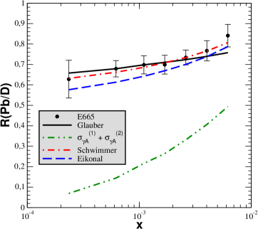
Figure 1: Comparison between the predictions of the distinct models and the E665 experimental data at small $x$.

III Numerical results and discussion

In what follows we shall consider two different nuclei, Ca and Pb, and use the deuteron (D) as a reference to calculate the experimentally measured ratios $R_{Ca/D}\equiv(2/40)F_{2}^{Ca}/F^{D}_{2}$ and $R_{Pb/D}\equiv(2/208)F^{Pb}_{2}/F^{D}_{2}$. We assume that the diffractive slope parameter is $B_{D}=6.7$ GeV^-2 and that the nucleus form factor is given by:

$$F_{A}(t_{\mathrm{min}})=\int d^{2}b\ J_{0}(b\sqrt{-t_{\mathrm{min}}})T_{A}(b),$$ (19)

where the thickness function is given in terms of the nuclear density $\rho_{A}$ as:

$$T_{A}(b)=\int_{-\infty}^{+\infty}dz\rho_{A}(\vec{b},z),$$

with the normalization fixed by $\int d^{2}b\ T_{A}(\vec{b})=1$.

In Fig. 1 we compare the predictions of the Glauber (solid line), Schwimmer (dot-dashed line), Eikonal (dashed line) and double scattering (dot-dot-dashed line) models for the ratios with the E665 experimental data at small $x$ e665 . Although joined with lines, our results are computed at the same $\langle x\rangle$ and $\langle Q^{2}\rangle$ as the experimental data. Our results demonstrate that if we compute the nuclear structure function up to two scatterings, which implies that $\sigma_{\gamma^{*}A}=\sigma_{\gamma^{*}A}^{(1)}+\sigma_{\gamma^{*}A}^{(2)}$, we are not able to describe the experimental data. Furthermore, since the magnitude of the first correction, $\sigma_{\gamma^{*}A}^{(2)}$, is very large, then there is no hope to estimate the nuclear structure function by just summing a few terms in the multiple scattering series. Therefore, a full resummation of the multiple scatterings is necessary, which makes the predictions model dependent. The agreement with the current experimental data at small $x$ of the Glauber, Schwimmer and Eikonal models is quite reasonable taking into account that no parameters have been fitted to reproduce the data. This implies that the current data are not able to discriminate between the unitarization schemes.

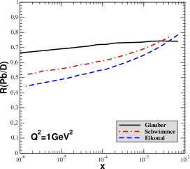
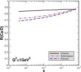
Figure 2: Nuclear ratios $R_{Pb/D}$ (left panel) and $R_{Ca/D}$ (right panel) as a function of $x$ at $Q^{2}=1$ GeV².

Having in mind that a future electron - ion collider is expected to be able to analyse the kinematical region of small $x$ ($x\simeq 10^{-5}$) and $Q^{2}\geq 1$ GeV², we now compute the ratios $R_{Ca/D}$ and $R_{Pb/D}$ as a function of $x$ for two different values of $Q^{2}$ (= 1 and 10 GeV²). In Fig. 2 we present our predictions for $Q^{2}=1$ GeV². It is important to emphasize that in electron scattering the range of $x$-values attainable is kinematically restricted to $x>Q^{2}/s$, where $s$ is the squared center-of-mass energy, which implies that at $Q^{2}=1$ GeV² the smaller values of $x$ in the perturbative region will be probed. At large $x$ ($\approx 10^{-2}$) the predictions almost coincide. However, at small $x$, the predictions based on the Schwimmer equation or on the eikonal unitarized cross section give a stronger shadowing than those based on Glauber-like rescatterings. In particular, at $x\approx 10^{-4}$, the difference between Glauber and Schwimmer is almost 10 % in the ratio $R(Ca/D)$ increasing to $\approx$ 20 % in $R(Pb/D)$. At this $x$ value, the difference between Schwimmer and Eikonal is $\approx$ 5 % and 12 % for the ratios $R(Ca/D)$ and $R(Pb/D)$, respectively. At smaller values of $x$, the difference between the three predictions increases, being larger than 20%. Consequently, a measurement of $F_{2}^{A}$ at $A=Pb$ at small $x$ with $\approx 10\%$ precision would be a sensitive test to discriminate between the different models.

In Fig. 3 we present our predictions for the ratios $R_{Ca/D}$ and $R_{Pb/D}$ as a function of $x$ at $Q^{2}=$ 10 GeV². The behavior is similar to the one observed in the Fig. 2. The main point is that the differences between the predictions is not reduced significantly and this makes the discrimination between them possible also at this value of $Q^{2}$.

A final comment is in order. The results shown in Figs. 2 and 3 demonstrate that there is a large uncertainty associated to the choice of unitarization scheme used to treat the multiple scatterings and that, in principle, an experimental analysis of the nuclear ratios can be useful to discriminate between these approaches.

Another uncertainty present in the study of the nuclear effects is related to the transition between the linear and nonlinear regimes of the QCD dynamics. We do not know precisely in which kinematical region the predictions obtained using the linear DGLAP evolution cease to be valid. In Fig. 4 we present a comparison of our predictions with those obtained using the EPS09 eps1 parametrization of the nuclear parton distribution functions, which is based on a global fit of the current nuclear data using the DGLAP dynamics. As it can be seen, due to the large theoretical uncertainty in the DGLAP prediction in the small-$x$ region, represented by the shaded band in the figure, it is not possible to draw any firm conclusion about which is the correct framework to describe this observable in future $eA$ colliders. This same conclusion was already obtained in erike_inclusive in a somewhat different approach. Consequently, the study of other observables, such as the nuclear diffractive structure function simone_eA ; raju_eA and nuclear vector meson production erike_exclusive ; vector_eA , should also be considered in order to discriminate between the linear and nonlinear regimes. To summarize: in order to learn more about the unitarization schemes using the nuclear ratios we must disentangle the nonlinear and linear regimes of the QCD dynamics. Our estimates show that due to the large freedom present in the DGLAP analysis they predict similar magnitudes for the nuclear ratios, which implies that a combined analysis of several observables is necessary.

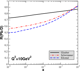
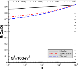
Figure 3: Nuclear ratios $R_{Pb/D}$ (left panel) and $R_{Ca/D}$ (right panel) as a function of $x$ at $Q^{2}=10$ GeV².

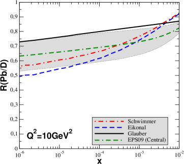
Figure 4: Predictions of the different models discussed in the text. The dash-dash-dot line represents the central value of the prediction obtained with the EPS09 parametrization of the nuclear parton distribution functions. The shaded band represents the theoretical error coming from the uncertainties in the EPS09 parametrization.

IV Conclusion

The behaviour of the nuclear wave function at high energies provides fundamental information for the determination of the initial conditions in heavy ion collisions and particle production in collisions involving nuclei. One of the main uncertainties is associated to the magnitude of the nuclear shadowing, which comes mainly from the way in which the multiple scattering problem is treated and from the modelling of the projectile - nucleon interaction. Since a future EIC will probe the shadowing region while keeping sufficiently large $Q^{2}$, new studies which determine the main sources of uncertainties in the predictions are necessary. In this work we compare three frequently used approaches to estimate the nuclear shadowing in nuclear DIS. As in these approaches the nuclear cross section is completely determined once the interaction of the projectile with the nucleon is specified, we considered a single model (rcBK) as input of our calculations in order to quantify the theoretical uncertainty which comes from the choice of the unitarization model. In particular, we calculate the nuclear ratio between structure functions considering the Glauber, Schwimmer and Eikonal approaches down to very low-$x$ utilizing the rcBK results both for inclusive and diffractive cross sections in $\gamma^{*}p$ scattering. Our results demonstrate that the current experimental data at small $x$ are described successfully by the three approaches. However, the difference between their predictions becomes large in the kinematical region which will be probed in the future electron - ion colliders.

V Acknowledgments

This work was partially financed by the Brazilian funding agencies CAPES, CNPq and FAPESP.

References

- (1) N. Armesto, J. Phys. G 32, R367 (2006).
- (2) L. Frankfurt, V. Guzey and M. Strikman, Phys. Rept. 512, 255 (2012).
- (3) M. R. Adams et al. [E665 Collaboration], Z. Phys. C 67, 403 (1995).
- (4) D. Boer, M. Diehl, R. Milner, R. Venugopalan, W. Vogelsang, D. Kaplan, H. Montgomery and S. Vigdor et al., arXiv:1108.1713 [nucl-th].
- (5) J.L. Abelleira Fernandez et al. [LHeC Study Group Collaboration], J. Phys. G 39, 075001 (2012).
- (6) K. J. Eskola, V. J. Kolhinen and P. V. Ruuskanen, Nucl. Phys. B 535, 351 (1998).
- (7) K. J. Eskola, V. J. Kolhinen and C. A. Salgado, Eur. Phys. J. C 9, 61 (1999).
- (8) M. Hirai, S. Kumano and T. H. Nagai, Phys. Rev. C 76, 065207 (2007).
- (9) D. de Florian and R. Sassot, Phys. Rev. D 69, 074028 (2004); D. de Florian, R. Sassot, P. Zurita and M. Stratmann, Phys. Rev. D 85, 074028 (2012).
- (10) K. J. Eskola, H. Paukkunen and C. A. Salgado, JHEP 0904, 065 (2009).
- (11) I. Helenius, K. J. Eskola, H. Honkanen and C. A. Salgado, JHEP 1207, 073 (2012).
- (12) F. Gelis, E. Iancu, J. Jalilian-Marian and R. Venugopalan, Ann. Rev. Nucl. Part. Sci. 60, 463 (2010);E. Iancu and R. Venugopalan, arXiv:hep-ph/0303204; H. Weigert, Prog. Part. Nucl. Phys. 55, 461 (2005); J. Jalilian-Marian and Y. V. Kovchegov, Prog. Part. Nucl. Phys. 56, 104 (2006).
- (13) N. Armesto, Eur. Phys. J. C 26, 35 (2002).
- (14) E. R. Cazaroto, F. Carvalho, V. P. Goncalves and F. S. Navarra, Phys. Lett. B 671, 233 (2009).
- (15) V. P. Goncalves, M. S. Kugeratski and F. S. Navarra, Phys. Rev. C 81, 065209 (2010).
- (16) V. P. Goncalves, M. S. Kugeratski, M.V.T. Machado and F. S. Navarra, Phys. Rev. C 80, 025202 (2009); E. R. Cazaroto, F. Carvalho, V. P. Goncalves, M. S. Kugeratski and F. S. Navarra, Phys. Lett. B 696, 473 (2011).
- (17) R. J. Glauber, in Lecture in Theoretical Physics, Vol. 1, edited by W. E. Brittin, L. G. Duham (Interscience, New York, 1959).
- (18) V. N. Gribov, Sov. Phys. JETP 29, 483 (1969); Sov. Phys. JETP 30, 709 (1970).
- (19) R. Venugopalan, Acta Phys. Polon. B 30, 3731 (1999).
- (20) A. Capella, A. Kaidalov, C. Merino, D. Pertermann and J. Tran Thanh Van, Eur. Phys. J. C 5, 111 (1998).
- (21) L. Frankfurt, V. Guzey, M. McDermott and M. Strikman, JHEP 0202, 027 (2002); L. Frankfurt, V. Guzey and M. Strikman, Phys. Rev. D 71, 054001 (2005); L. Frankfurt, V. Guzey and M. Strikman, Phys. Lett. B 586, 41 (2004).
- (22) N. Armesto, A. Capella, A. B. Kaidalov, J. Lopez-Albacete and C. A. Salgado, Eur. Phys. J. C 29, 531 (2003).
- (23) N. Armesto, A. B. Kaidalov, C. A. Salgado and K. Tywoniuk, Eur. Phys. J. C 68, 447 (2010).
- (24) V. N. Gribov, Sov. Phys. JETP 26, 414 (1968).
- (25) V. A. Abramovsky, V. N. Gribov and O. V. Kancheli, Yad. Fiz. 18, 595 (1973) [Sov. J. Nucl. Phys. 18, 308 (1974)].
- (26) A. Schwimmer, Nucl. Phys. B 94, 445 (1975).
- (27) B. Z. Kopeliovich, J. Raufeisen and A. V. Tarasov, Phys. Lett. B 440, 151 (1998); B. Z. Kopeliovich, J. Raufeisen and A. V. Tarasov, Phys. Rev. C 62, 035204 (2000); J. Nemchik, Phys. Rev. C 68, 035206 (2003).
- (28) N. Armesto, A. B. Kaidalov, C. A. Salgado and K. Tywoniuk, Phys. Rev. D 81, 074002 (2010).
- (29) I. Balitsky, Nucl. Phys. B 463, 99 (1996); Y. V. Kovchegov, Phys. Rev. D 60, 034008 (1999); Phys. Rev. D 61, 074018 (2000).
- (30) J. L. Albacete, N. Armesto, J. G. Milhano and C. A. Salgado, Phys. Rev. D 80, 034031 (2009).
- (31) M. A. Betemps, V. P. Goncalves and J. T. de Santana Amaral, Eur. Phys. J. C 66, 137 (2010).
- (32) J. L. Albacete and C. Marquet, Phys. Lett. B 687, 174 (2010).
- (33) V. P. Goncalves, M. V. T. Machado and A. R. Meneses, Eur. Phys. J. C 68, 133 (2010).
- (34) N. N. Nikolaev and B. G. Zakharov, Z. Phys. C49, 607 (1991); Z. Phys. C53, 331 (1992).
- (35) K. J. Golec-Biernat and M. Wusthoff, Phys. Rev. D 59, 014017 (1998), ibid. D60, 114023 (1999).
- (36) M. Wusthoff, Phys. Rev. D 56, 4311 (1997).
- (37) N. N. Nikolaev and B. G. Zakharov, J. Exp. Theor. Phys. 78, 598 (1994); Z. Phys. C64, 631 (1994); N. N. Nikolaev, W. Schaefer, B. G. Zakharov and V. R. Zoller, JETP Lett. 80, 371 (2004).
- (38) J. R. Forshaw, R. Sandapen and G. Shaw, Phys. Lett. B 594, 283 (2004).
- (39) C. Marquet, Phys. Rev. D 76, 094017 (2007).
- (40) E. Iancu, A. Leonidov, L. McLerran, Nucl. Phys. A 692, 583 (2001); E. Ferreiro, E. Iancu, A. Leonidov, L. McLerran, Nucl. Phys. A 703, 489 (2002); J. Jalilian-Marian, A. Kovner, L. McLerran and H. Weigert, Phys. Rev. D 55, 5414 (1997); J. Jalilian-Marian, A. Kovner and H. Weigert, Phys. Rev. D 59, 014014 (1999), ibid. 59, 014015 (1999), ibid. 59 034007 (1999); A. Kovner, J. Guilherme Milhano and H. Weigert, Phys. Rev. D 62, 114005 (2000); H. Weigert, Nucl. Phys. A703, 823 (2002).
- (41) L. N. Lipatov, Sov. J. Nucl. Phys. 23, 338 (1976); E. A. Kuraev, L. N. Lipatov, V. S. Fadin, JETP 45, 1999 (1977); I. I. Balitskii, L. N. Lipatov, Sov. J. Nucl. Phys. 28, 822 (1978).
- (42) Y. V. Kovchegov and H. Weigert, Nucl. Phys. A 784, 188 (2007); Nucl. Phys. A 789, 260 (2007); Y. V. Kovchegov, J. Kuokkanen, K. Rummukainen and H. Weigert, Nucl. Phys. A 823, 47 (2009).
- (43) J. L. Albacete and Y. V. Kovchegov, Phys. Rev. D 75, 125021 (2007).
- (44) I. Balitsky, Phys. Rev. D 75, 014001 (2007); I. Balitsky and G. A. Chirilli, Phys. Rev. D 77, 014019 (2008).
- (45) J. Kuokkanen, K. Rummukainen and H. Weigert, Nucl. Phys. A 875, 29 (2012).
- (46) M. S. Kugeratski, V. P. Goncalves and F. S. Navarra, Eur. Phys. J. C 46, 413 (2006)
- (47) H. Kowalski, T. Lappi and R. Venugopalan, Phys. Rev. Lett. 100, 022303 (2008); H. Kowalski, T. Lappi, C. Marquet and R. Venugopalan, Phys. Rev. C 78, 045201 (2008)
- (48) A. Caldwell and H. Kowalski, Phys. Rev. C 81, 025203 (2010); T. Lappi and H. Mantysaari, Phys. Rev. C 83, 065202 (2011)