On the structure of molecular clouds

Abstract

We show that the inter-cloud Larson scaling relation between mean volume density and size $\rho\propto R^{-1}$, which in turn implies that mass $M\propto R^{2}$, or that the column density $N$ is constant, is an artifact of the observational methods used. Specifically, setting the column density threshold near or above the peak of the column density probability distribution function $N$-pdf ($N\sim 10^{21}$ cm^-2) produces the Larson scaling as long as the $N$-pdf decreases rapidly at higher column densities. We argue that the physical reasons behind local clouds to have this behavior are that (1) this peak column density is near the value required to shield CO from photodissociation in the solar neighborhood, and (2) gas at higher column densities is rare because it is susceptible to gravitational collapse into much smaller structures in specific small regions of the cloud. Similarly, we also use previous results to show that if instead a threshold is set for the volume density, the density will appear to be constant, implying thus that $M\propto R^{3}$. Thus, the Larson scaling relation does not provide much information on the structure of molecular clouds, and does not imply either that clouds are in Virial equilibrium, or have a universal structure. We also show that the slope of the $M-R$ curve for a single cloud, which transitions from near-to-flat values for large radii to $\alpha=2$ as a limiting case for small radii, depends on the properties of the $N$-pdf.

1 Introduction

More than 30 years ago, Larson (1981) published his scaling relations for molecular clouds (MCs): the column density-size relation (or “Larson’s third relation”)

$$\rho\propto R^{\gamma_{1}}$$ (1)

and the velocity dispersion-size relation

$$dv\propto R^{\gamma_{2}}.$$ (2)

The exponents reported in that work were $\gamma_{1}=-1.1$ and $\gamma_{2}=0.39$, respectively. However, the more widely accepted values are $\gamma_{1}=-1$ and $\gamma_{2}=0.5$; and these have been usually thought to be observational evidence that clouds are in Virial equilibrium, although it is important to recall that any pair $(\gamma_{1},\gamma_{2})$ satisfying $\gamma_{1}=2\gamma_{2}-2$ will be consistent with Virial equilibrium (see e.g., Vázquez-Semadeni & Gazol, 1995).

Larson’s relations have been used in many papers to describe the internal structure of clouds (e.g., Goldbaum et al., 2011, to cite just one of the more recent examples). However, their validity has been called into question for observational reasons (Kegel, 1989; Scalo, 1990; Vázquez-Semadeni et al., 1997; Ballesteros-Paredes & Mac Low, 2002; Ballesteros-Paredes, 2006; Ballesteros-Paredes et al., 2011a). Specifically, clouds should have a minimum column density to be detected; and if the column density where too large, clouds will become optically thick (in ¹²CO), and then such dense regions would not be easily detected. The net result of these effects would be that observed CO clouds should exhibit a small dynamic range in column density, independent of their intrinsic structure.

In a recent study, Lombardi et al. (2010) used near-infrared extinction measurements to increase the dynamic range of inferred mass column densities. They studied a sample of local MCs with substantially different physical properties, from giant MCs hosting massive star formation, and masses of the order of 2$\times 10^{5}$ $M_{\odot}$(e.g., Orion), down to clouds with less star formation activity, and masses of the order of several thousand $M_{\odot}$ (the Pipe Nebula). Their main results are:

• For an ensemble of MCs observed at a given extinction threshold $A_{0}$, the mass varies with size as $M\propto R^{2}$, implying that the column density $\Sigma=N/\mu m_{H}$ is constant and depends on that threshold.

• The numerical value of the column density changes with the value of the threshold $A_{0}$.

• When analyzing a single MC at different thresholds $A_{0}$, the mass-size relation varies as a power-law, with a somewhat shallower power law index ($M\propto r^{1.6}$).

Lombardi et al. (2010) argue that their results can be understood as a consequence of the fact that clouds exhibit a column density probability distribution function ($N$-pdf) with a lognormal functional form, although in a recent paper, Beaumont et al. (2012) revisit the Lombardi et al. (2010) analysis, and suggest (without demonstration) that other forms than a lognormal $N$-pdf can produce the same result. They also argue that the only requirement to satisfy Larson’s third relation is that the mean $N$-pdf is uncorrelated with region-to-region dispersion in area.

In the present work we discuss why MCs with very different properties appear to have very similar column densities at a given threshold. In §2 we draw $\Sigma-A_{0}$ diagrams to show that the main features found by Lombardi et al. (2010) are found for very different functional forms, and that the scatter in column density at any threshold is smaller than a factor of 3. In §4 we show, furthermore, that when thresholding the volume density, what appears to be constant is the volume density, suggesting that the relation is a consequence of the procedure adopted. We argue that the only special feature of the structure of local MCs is that they peak at a particular value of the mean $N$-pdf, in agreement with Beaumont et al. (2012). In §5, we analyze the case of the mass-size relation for a single cloud, showing that rather than a power-law, the relation is a curve that has slope approaching to 2 at small radii, and flattens for larger radius. As a consequence, there is some interval in which the slope is close to 1.6-1.7, as reported in observations. The properties of this relation are determined directly by the shape of the $N$-pdf. In §6 we further identify the physical reasons for having a typical $N$-pdf: First, there is a minimum column density for CO shielding; and second, above this threshold the amount of mass decreases rapidly with increasing column density, which is probably the result of gravitational contraction and collapse.

2 Formalism: Column density PDFs and their $\Sigma-A_{0}$ diagram

In our analysis we follow the formalism outlined by Lombardi et al. (2010). We use $A$ to denote the extinction in the $K$ band unless otherwise specified. We also recall that $A_{V}\sim 10A_{K}$, and that the $N$-pdf published by Kainulainen et al. (2009) have a peak at $A_{k}\sim$ 0.1, equivalent to $A_{V}\sim 1$ or $N\sim 10^{21}$ cm^-2. Now, given a probability distribution function of the extinction $p(A)dA$, the area and mass above some extinction threshold $A_{0}$ are defined as:

$$S(A_{0})=S_{\rm tot}\ \int_{A_{0}}^{\infty}\ p(A)\ dA$$ (3)

and

$$M(A_{0})=S_{\rm tot}\mu m_{H}\ \beta\int_{A_{0}}^{\infty}A\ p(A)\ dA,$$ (4)

where $\mu$ is the mean molecular weight within the MC, $m_{H}$ is the mass of the hydrogen atom, and $\beta$ is the ratio between the total hydrogen column density and the dust extinction coefficient. Lombardi et al. (2010, see their Fig 4) showed that if clouds have a lognormal $N$-pdf, the surface density as a function of $A_{0}$, which is given by the ratio of eq. (4) divided by eq. (3), is nearly constant for low thresholds $A_{0}$, and varies approximately linearly for large thresholds, i.e.,

$$\Sigma=\ \left\{\begin{array}[]{rl}\to{\rm constant}&\mbox{if $A_{0}<<A_{\rm max}$,}\\ \propto A_{0}&\mbox{if $A_{0}>>A_{\rm max}$,}\end{array}\right.$$ (7)

where $A_{\rm max}$ is the extinction value at which the $N$-pdf peaks. Since this behavior reproduces qualitatively that of the 12 MCs in the Solar neighborhood they analyzed, these authors suggest that the observed constancy of the column density for different clouds is due to their intrinsic internal structure, given by a lognormal $N$-pdf. However, many of the MCs in the solar neighborhood do not exhibit a lognormal $N$-pdf at large column densities but rather frequently exhibit power-law or more complicated shapes (Froebrich et al., 2007). Thus, the behavior of $\Sigma(A_{0})$ described above cannot be consequence of a universal distribution function of the column density of the MCs.

In order to understand the origin of Larson’s third relation for multiple clouds, we analyze the following examples. For clarity’s sake, we will first describe the examples, leaving the discussion for §3.6.

3 The Inter-cloud mass-size relation for simple column density pdfs

3.1 A single power-law

First, assume that the $N$-pdf has a power-law shape:

$$p(A)dA=p_{0}(A/A_{\rm max})^{-n}dA$$ (8)

Using this equation, the mass above some extinction threshold is given by

$$M(A_{0})=-{{S_{\rm tot}}\mu m_{H}\beta p_{0}A_{\rm max}^{2}\over 2-n}\biggl{(}{A_{0}\over A_{\rm max}}\biggr{)}^{2-n},$$ (9)

were we have assumed that $n>2$ in order to get a finite mass (indeed, by simple inspection one can verify that all the column density histograms of MCs published in the literature fall faster than a power-law with an exponent of $m\geq 2.5$, i.e., $n\geq 3.5$, see e.g., Kainulainen et al., 2009). Similarly, the area of the cloud will be given by

$$S(A_{0})=-{{S_{\rm tot}}p_{0}A_{\rm max}\over 1-n}\biggl{(}{A_{0}\over A_{\rm max}}\biggr{)}^{1-n}$$ (10)

and thus, the column density will be simply given by

$$\Sigma\equiv{M(A_{0})\over S(A_{0})}=\mu m_{H}\beta A_{\rm max}\biggl{(}{1-n\over 2-n}\biggr{)}\biggl{(}{A_{0}\over A_{\rm max}}\biggr{)}.$$ (11)

We note then, that for a power-law distribution, the column density always varies linearly with $A_{0}$ (see also Beaumont et al., 2012).

3.2 Two power laws

Now assume that the $N$-pdf has a two power-law shape: one with a positive exponent, for low extinctions, and the other with a negative exponent, for large extinctions, i.e.,

$$p(A)=\left\{\begin{array}[]{rl}p_{0}(A/A_{\rm max})^{q}&\mbox{for $A\leq A_{\rm max}$,}\\ p_{0}(A/A_{\rm max})^{-n}&\mbox{for $A\geq A_{\rm max}$,}\end{array}\right.$$ (14)

with $q,n>0$. Plugging this $N$-pdf into eqs. (3) and (4) we obtain

$$S=K_{1}\biggl{\{}{1\over 1+q}\biggl{[}1-\biggl{(}{A_{0}\over A_{\rm max}}\biggr{)}^{1+q}\biggr{]}-{1\over 1-n}\biggr{\}}$$ (15)

with

$$K_{1}={S_{\rm tot}}p_{0}A_{\rm max}$$ (16)

and

$$M=K_{2}\biggl{\{}{1\over 2+q}\biggl{[}1-\biggl{(}{A_{0}\over A_{\rm max}}\biggr{)}^{2+q}\biggr{]}-{1\over 2-n}\biggr{\}}$$ (17)

with

$$K_{2}={S_{\rm tot}}\mu m_{H}\beta p_{0}A_{\rm max}^{2}.$$ (18)

Making $K_{3}=K_{2}/K_{1}=\mu m_{H}\beta A_{\rm max}$, the surface density is given by

$$\Sigma(A_{0})=K_{3}{\biggl{[}1-\bigl{(}{A_{0}/A_{\rm max}}\bigr{)}^{2+q}\biggr{]}{(2+q)^{-1}}-(2-n)^{-1}\over\biggl{[}1-\bigl{(}{A_{0}/A_{\rm max}}\bigr{)}^{1+q}\biggr{]}{(1+q)^{-1}}-(1-n)^{-1}}$$ (19)

for $A_{0}\leq A_{\rm max}$. For larger $A_{0}$, the case is reduced to a single power-law, and the surface density will be given by eq. (11).

In Fig. 1 we plot $\Sigma$ vs $A_{0}$ for a two power-law $N$-pdf. In both cases, we have assumed $A_{\rm max}=0.1$, the typical value found in a large sample of Solar neighborhood MCs by Kainulainen et al. (2009). In the upper panel we vary $n$ from $\sim 3.8$ to 5.8, in steps of 0.5. This is approximately the range of exponents that can be found in the $N$-pdfs presented by Kainulainen et al. (2009, $m\sim 2.8$ to 4.8.) As expected, the change in the power-law index modifies the surface density at every $A_{0}$. In the lower panel, however, varying the low-extinction index $q$ (from 0 to 4.5 in steps of 0.5) only modifies the surface density for low $A_{0}$.

Figure 1: $\Sigma$ vs $A_{0}$, from cloud $N$-pdfs given by two power laws, as in eq. (14). The upper panel presents curves with $q=0$ and $n=2.8$, 3.3, 3.8, 4.3, and 4.8. Lower panel: curves with $n=$, and $q=1$ to 5.5 in steps of 0.5. Note that in both cases, the inferred column density $\Sigma$ is the same, within a factor of $\sim$2.

Two more features can be inferred at this point. First of all, for large $A_{0}$, this case is reduced to the previous one (a single power-law), and then, the column density varies linearly with the extinction threshold, i.e., $\Sigma\propto A_{0}$. On the other hand, at low $A_{0}$ ($<<A_{\rm max}$), the column density for a cloud with a given $N$-pdf becomes constant:

$$\Sigma(A_{0})\simeq\mu m_{H}\beta A_{\rm max}\biggl{(}{1+q\over 2+q}\biggr{)}\biggr{(}{1-n\over 2-n}\biggr{)}.$$ (20)

We notice, moreover, that for typical values of $n,q$, the minimum column density given by eq. (20) varies less than a factor of two.

3.3 A lognormal $N$-pdf

The case of a lognormal $N$-pdf was analyzed by Lombardi et al. (2010), and the mass surface density is given by

$$\Sigma(A_{0}) = \mu m_{H}\beta A_{\rm max}\exp\biggl{(}{\sigma^{2}\over 2}\biggr{)}\times$$ (21)

$${1-{\rm erf}\{[\ln{(A_{0}/A_{\rm max})}-\sigma^{2}]/\sqrt{2}\sigma\}\over 1-{\rm erf}[\ln{(A_{0}/A_{\rm max})}/\sqrt{2}\sigma]}.$$

Although the non-dimensional plot of this function has been already presented and discussed by these authors, for comparison we display it in dimensional form, assuming $A_{\rm max}=0.1$. The qualitative behavior is similar to that of the $N$-pdf exhibiting two power-laws previously discussed.

Figure 2: $\Sigma$ vs $A_{0}$, for a cloud that exhibits a $N$-pdf given by a lognormal function. Here we assume $A_{\rm max}=0.1$. The different curves follow eq. (21) with $\sigma=0.29$ and 0.59 (the range of variation in $\sigma$ for the lognormal functions fitted by Kainulainen et al., 2009), plus two extreme cases: $\sigma=1$, and 1.5. We note that, even for these unrealistic cases, the inferred column density $\Sigma$ is the quite the same, within a factor of $\leq$ 3–5.

We further note that, since the error function can be expanded as

$${\rm erf}(x)\simeq 1-{\exp{(-x^{2})}\over\sqrt{\pi}}\biggl{(}x^{-1}-{1\over 2}x^{-3}+{3\over 4}x^{-5}+...\biggr{)},$$ (22)

to first order the mass column density can be written as:

$$\Sigma = \mu m_{H}\beta A_{\rm max}\exp{\biggl{(}{\sigma^{2}\over 2}\biggr{)}}\ln(A_{0}/A_{\rm max})\times$$

$$\biggl{(}{\exp{[-{(\ln({A_{0}/A_{\rm max}})-\sigma^{2})^{2}/\sqrt{2}\sigma}]}\over(\ln({A_{0}/A_{\rm max}})-\sigma^{2})\exp{[-\ln({A_{0}/A_{\rm max}})/2\sigma^{2}]}}\biggr{)},$$

for large values of $A_{0}$. Simplifying,

$$\Sigma=\mu m_{H}\beta A_{\rm max}{({A_{0}/A_{\rm max}})\ln{(A_{0}/A_{\rm max})}\over\ln{(A_{0}/A_{\rm max})}-\sigma^{2}}.$$ (23)

This equation makes clear that, for large $A_{0}/A_{\rm max}$, $\ln(A_{0}/A_{\rm max})>>\sigma^{2}$ and thus,

$$\Sigma\propto A_{0}.$$ (24)

On the other hand, for small $A_{0}$, $\Sigma$ becomes constant with a value of

$$\Sigma(A_{0})=\mu m_{H}\beta A_{\rm max}\exp{\sigma^{2}\over 2}.$$ (25)

3.4 Column density PDF with several peaks

We now proceed with a slightly more complicated example: a three-peaked $N$-pdf defined by three lognormal functions, as follows.

$$p(A)dA=\sum_{i=1,3}{p_{i}\over A}\exp{\biggl{(}-{(\ln A-\ln A_{i})^{2}\over 2\sigma_{i}^{2}}\biggr{)}}dA,$$ (26)

and thus, the surface density will be given by

$$\Sigma = {\mu m_{H}\beta\over\sqrt{2\pi}}\times\biggl{\{}$$ (27)

$${\sum_{i=1,3}p_{i}A_{i}e^{\sigma_{i}^{2}/2}\bigl{[}1-{\rm erf}\bigl{(}(\sigma_{i}-\ln{(A_{0}/A_{i})})/\sqrt{2}\sigma_{i}\bigr{)}\bigr{]}}/$$

$${\sum_{i=1,3}p_{i}\sigma_{i}\bigl{[}1-{\rm erf}[\ln{(A_{0}/A_{i})}/\sqrt{\sigma}_{i}]\bigr{]}}\biggr{\}}$$

In Fig 3 we show our hypothetical $N$-pdf (upper panel), and its respective $\Sigma$ vs $A_{0}$ function (lower panel). The parameters of the lognormal functions were chosen to enhance their effect on the column density. In reality, the observed $N$-pdfs exhibit smaller variations. As can be noted from this figure, we again reproduce the main features observed in the $\Sigma-A_{0}$ diagram: for $A_{0}>>A_{1}$, $\Sigma$ increases linearly with $A_{0}$, and for for $A_{0}<<A_{1}$, $\Sigma$ becomes constant. Additionally, in this case we note that the peaks in the $N$-pdf produce small fluctuations with a trend that has a slope close, but smaller than unity. We will get back to such fluctuations below.

Figure 3: Upper panel: $N$-pdf of a hypothetical MC exhibiting three peaks. Lower panel: its corresponding $\Sigma$ vs $A_{0}$ diagram. The dotted line denotes the line with slope $\beta_{K}^{-1}$, where $\beta=1.67\times 10^{22}$cm^-2 mag^-1, the opacity in the $K$ band.

3.5 Lognormal with a power-law tail PDF

Most of the observed column density histograms appear to behave as a lognormal function, at low extinctions, with a power-law tail, at larger $A$ (e.g., Kainulainen et al., 2009, see also Ballesteros-Paredes et al. 2011b for the theoretical counterpart). The functional form of such $N$-pdf is, thus,

$$p(A)dA=\left\{\begin{array}[]{rl}p_{0}\exp{\biggl{(}-{(\ln A-\ln A_{\rm max})^{2}\over 2\sigma^{2}}\biggr{)}}dA/A&\mbox{if $A\leq A_{\rm cut}$,}\\ p_{1}({A/A_{\rm cut}})^{-n}dA&\mbox{if $A\geq A_{\rm cut}$,}\end{array}\right.$$ (30)

where $\ln{A_{\rm max}}$ denotes the extinction value at which the lognormal is maximum, and $\ln{A_{\rm cut}}$ the place where the $N$-pdf changes from a lognormal to a power-law function. The continuity condition at $A_{\rm cut}$ is:

$$p_{1}=\biggr{(}{p_{0}\over A_{\rm cut}}\biggr{)}\exp\biggl{(}-{(\ln A_{\rm cut}-\ln A_{\rm max})^{2}\over 2\sigma^{2}}\biggr{)}.$$ (31)

As in the case of two power-laws (§3.2), at large extinctions ($A>A_{2}$), the mass, surface and column density must be given by the solution of a single powerlaw, eqs. (9), (10) and (11). For smaller extinctions ($A<A_{\rm cut}$), however, the solutions for $M$ and $S$ are:

$$S(A_{0})=S_{\rm tot}\biggl{\{}p_{0}\sqrt{\pi\over 2}\sigma\biggl{[}{\rm erf}\biggl{(}{\ln(A_{\rm cut}/A_{\rm max})\over\sqrt{2}\sigma}\biggr{)}-$$

$${\rm erf}\biggl{(}{\ln(A_{0}/A_{\rm max})\over\sqrt{2}\sigma}\biggr{)}\biggr{]}-{p_{1}A_{\rm cut}\over 1-n}\biggr{\}},$$ (32)

and

$$M(A_{0})=S_{\rm tot}\mu m_{H}\beta\ \biggl{\{}-p_{0}\sqrt{\pi\over 2}\sigma{\rm e}^{\sigma^{2}/2}A_{\rm max}$$

$$\biggl{[}{\rm erf}\biggl{(}{\sigma^{2}-\ln A_{\rm cut}+\ln{A_{\rm max}}\over\sqrt{2}\sigma}\biggr{)}-$$

$${\rm erf}\biggl{(}{\sigma^{2}-\ln A_{0}+\ln A_{\rm max}\over\sqrt{2}\sigma}\biggr{)}\biggr{]}-$$

$${p_{1}A^{2}_{\rm cut}\over 2-n}\biggr{\}},$$ (33)

while the column density is given by the ratio of eqs. (33) over (32). We now plot the $N$-pdf as a function of the extinction $A$ (upper panels), and its corresponding mass column density $\Sigma$ as a function of the extinction threshold $A_{0}$ (lower panels). In Fig. 4 we vary the value of $A_{\rm cut}$, the extinction value where we the power-law cuts the lognormal. In fig. 5 we vary the value of the power-law index $n$, while in Fig. 6 we vary the value of the standard deviation $\sigma$ of the lognormal function.

As we can see, again, the column density is basically the same in all cases, regardless of the parameter we are varying, and large differences occur only when we strongly vary the power-law index $n$.

Figure 4: Upper panel: $N$-pdf defined by a lognormal function at low extinctions and a power-law tail at large extinctions, for different values of $A_{\rm cut}$: 0.2, 0.3, and 0.4. $\Sigma=0.4$ and $n=4$ ($m=3$) remain fixed. Lower panel: The corresponding $\Sigma-A_{0}$ diagram. Notice that in the power-law regime ($A>A_{\rm cut}$), the column density is the same for the three cases, since they have the same value of $n$ and $A_{\rm cut}$, (see eq. (11)).

Figure 5: Upper panel: $N$-pdf defined by a lognormal function at low extinctions and a power-law tail at large extinctions, for different values of $n$: 3, 4, 5, and 6. $\Sigma=0.4$ and $A_{2}=0.2$ remain fixed. Note that the slope that one measures in this plot is $m=n-1$. Lower panel: The corresponding $\Sigma-A_{0}$ diagram.

Figure 6: Upper panel: $N$-pdf defined by a lognormal function at low extinctions and a power-law tail at large extinctions, for different values of $\sigma$: 0.3, 0.4, 0.5, 0.6, and the unrealistic cases with $\sigma=$1 and 1.5. $A_{2}=0.3$ and $n=4$ ($m=3$) remain fixed. Lower panel: The corresponding $\Sigma-A_{0}$ diagram. As in the case of Fig. 4, the column density in the power-law regime ($A>A_{\rm cut}$) is the same for the three cases, since they have the same value of $n$ and $A_{\rm cut}$.

3.6 Conclusions from the $\Sigma-A_{0}$ diagrams

In the previous sections we have constructed different functional forms of the $N$-pdf. Their main features are: (i) they peak at the same value ($A_{1}\sim 0.1$), (ii) and they decrease strongly for larger extinction values. In all cases we have recovered the main two features observed for the column density of MCs: at low extinction thresholds, the column density is nearly constant, while at large extinction thresholds the column density increases linearly with the threshold. Additionally, in all cases the values obtained for $\Sigma$ at any $A_{0}$ are quite similar, despite their strong differences in functional form of the $N$-pdf.

The reason for which very different $N$-pdfs produce approximately the same values of the observed column density at a given threshold, appearing to reproduce the $M\propto R^{2}$ relation, is a consequence of the definition of $\Sigma$ itself, along with the fact that the $N$-pdfs of MCs decay fast: the column density given by the ratio of eq. (4) over eq. (3) is the average of the extinction coefficient (which is proportional to the mean surface density) above the extinction threshold $A_{0}$. Lets assume now that the $N$-pdf has an arbitrary shape below its maximum at $A_{1}$, and decreases strongly beyond that value. For $A_{0}<A_{1}$, the mean column density does not change substantially with the threshold $A_{0}$ because the mass at a given extinction $A$, which is proportional to the product of the number of points contributing to the $N$-pdf times $A$, ($dm\propto ApdA$), will be dominated by the mass at the peak $A_{1}$. Note that this is valid even if the $N$-pdf were flat for $A_{0}<A_{1}$. This is the case where the surface density is constant with $A_{0}$ in the $\Sigma-A_{0}$ diagram.

As we approach the peak of the $N$-pdf, small changes in the threshold $A_{0}$ start removing a substantial number of low extinction data points from the $N$-pdf. The calculation of our mean extinction starts to be dominated by larger values of $A$, making the mean surface density $\langle\Sigma\rangle$ to increase rapidly. Once we have passed the maximum $(A_{0}>A_{\rm max})$, and the distribution decreases rapidly, the mass will be dominated by values close -but above- to $A_{0}$. This is the range in which the $\langle\Sigma\rangle$ varies linearly with the threshold, i.e., $\langle\Sigma\rangle\propto A_{0}$.

A similar analysis can be performed if the $N$-pdf exhibits several bumps, as in the case of our three-peaked $N$-pdf (see Fig.3): below each peak, the $\Sigma-A_{0}$ curve is more or less constant because the mass is dominated by the next peak. After each peak, the column density grows fast because we are removing a substantial number of points at low column densities. Once we reach the final peak, the column density should increase proportional to $A_{0}$ because the mass is dominated by values slightly larger than $A_{0}$.

We emphasize that the arguments given by Kegel (1989) and Scalo (1990), that clouds are not seen at large column densities because of optically thick effects, do not apply because of the larger dynamic range available in more recent observations. Clouds approximately fall along the constant column density line just because we are measuring the mean value of a property which probability distribution function has a peak at nearly the same value for all objects, and falls fast enough.

On the other hand, from the present analysis it becomes clear how a molecular cloud must behave in order to depart from the Larson’s third relation, i.e., in order to have, at a given threshold, a substantially different column density compared to other clouds: (a) it must have a wider $N$-pdf, or (b) it must peak at a substantially different extinction value $A_{\rm max}$. The first case can be achieved by having either a $N$-pdf with a much flatter slope at large column densities, or a wider lognormal. Nevertheless, all the $N$-pdfs reported in the literature fall a factor of $\sim$ 3 orders of magnitude when increasing one order of magnitude in column density (Kainulainen et al., 2009), making this possibility inapplicable from the observational point of view. Moreover, it has been shown theoretically that, for a supersonic turbulent field with Mach number $M$, the volume density PDF has a standard deviation $\sigma_{\rho}$ given by

$$\sigma_{\log{\rho}}=\sqrt{\ln(1+M^{2}/4)}$$ (34)

(Ostriker et al., 1999; Padoan & Nordlund, 2002). Clearly, the dependence on $M$ is weak. If one takes one of the most extreme cases known, the G0.253$+$0.016 molecular cloud near the galactic center (Longmore et al., 2012), with a velocity dispersion of 16 km sec^-1, the width of the volume pdf will differ by only a factor of two from more typical clouds, like Taurus with a dispersion of $\sim 2$ km sec^-1. But the column density PDF by definition must have a smaller width, since the column density is the integral of the volume density, and thus, density fluctuations are smeared out. Thus, one should not expect a wide lognormal $N$-pdf even for large Mach numbers.

In the second case, i.e., for hypothetical clouds peaking at substantially different extinction values $A_{\rm max}$, if the dust opacity $\beta$ is the same for such a cloud, its $\Sigma-A_{0}$ curve will be shifted along the line with slope unity, increasing also its column density for $A_{0}<A_{\rm max}$, as shown in Fig. 7. From this figure, one may think that for extinction thresholds $A_{0}<1$, such a cloud will exhibit a much larger column density at a given threshold, compared to the Solar Neighborhood clouds. Although one may think that this could be the case of the infrared dark clouds (IRDCs), which achieve column densities substantially larger than local clouds with typical values of 10²² cm^-2 and maximum values up to 10²⁴ cm^-2 (e.g., Ragan et al., 2011), the cumulative mass functions of IRDCs Kainulainen et al. (2011, see their Fig. 7) show that the mass keeps increasing moving to lower extinction $A_{V}\sim 2$, indicating that the peak of their $N$-pdf must be at $A_{v}\sim 1-2$, just as local clouds.

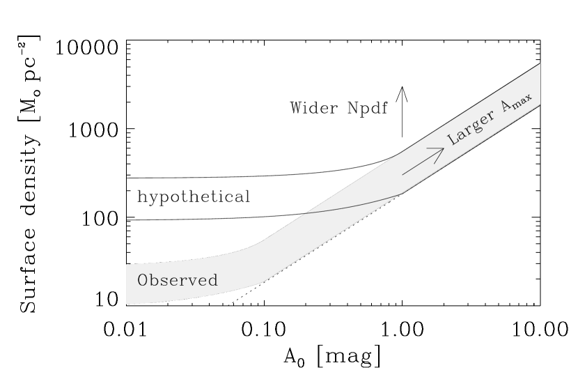
Figure 7: Schematic $\Sigma-A_{0}$ diagram for local clouds (shadow region), and for some hypothetical clouds (white region). Note that, the wider the $N$-pdf, the wider the gray region. If the dust opacity of such hypothetical clouds is the same than that of the local clouds, their locus in this diagram should be shifted towards the upper right region, as indicated. Here we assumed that $A_{\rm max}\sim 1$ for these clouds. Observed $N$-pdf of IRDCs by Kainulainen et al. (2011) discard the possibility of these clouds.

4 The effect of thresholding density

Imagine now that we were able to measure the volume density fields of MCs, and then threshold them in order to measure the mean volume density of the clouds. In this case, what we would obtain is a nearly constant volume density, implying that $M\propto R^{3}$. To show that this is the case, in Fig. 8 we show the volume density ($y$ axis) against size ($x$ axis) for clumps in a numerical simulation of isothermal molecular clouds with forced turbulence, as published by Ballesteros-Paredes & Mac Low (2002, Fig. 9). The details of the particular simulation used and on the assumptions used for the radiative transfer performed to mimic the line emission can be found in that paper. Here we stress that the same result can be found in simulations with or without self-gravity, with or without magnetic fields, or whether the turbulence is forced or decaying. The data points in the upper panel are obtained by thresholding the volume density, while the middle and lower panels are obtained by thresholding the simulated CS(1-0) and the ¹³CO(1-0) intensity, respectively, which is proportional to the column density. The dotted line in these panels has a slope of $-1$, i.e., its a line with constant column density.

Figure 8: Density-size relation for clumps in numerical simulations. Upper panel: real space, or position-position-position (PPP) space. The clumps are found by thresholding the volume density field. Middle and lower panels: observational space, position-position-velocity (PPV) space. In this case, the clumps are found by thresholding the intensity, which in turn is proportional to the column density. Figure taken from Ballesteros-Paredes & Mac Low (2002).

It can be seen from the upper panel that the volume density seems to be constant for all cores, when we threshold the volume density. When we analyze the observational space (middle and lower panels), the points follow the straight line with slope $-1$, implying that the column density is constant. In this case, the cores were found by thresholding the intensity, which is proportional to the column density. Thus, while we will deduce a relation $M\propto R^{3}$ from the upper panel, from the lower two we will deduce that the relation is $M\propto R^{2}$.

5 The intra-cloud mass-size relation

We now turn to the intra-cloud mass-size relation, i.e., the $M-R$ relation for a single cloud. In this case, Fig. 2 by Lombardi et al. (2010) show that none of the $M-R$ diagrams exhibit a power-law of the form:

$$M\propto R^{a},$$ (35)

Instead, the $M-R$ diagram of all clouds is a curved line with the following properties: (a) at the smaller radii, all curves exhibit a power-law with slope of 2, and (b) for the larger radii, all the curves become flatter, with slopes of the order of unity. A natural consequence of these properties is that there is a region at intermediate radii (between 0.3 and 3 pc) where the curve can be fitted by a power-law with an exponent of $a\sim$1.6-1.7. This is the observational result quoted by Kauffmann et al. (2010) and Lombardi et al. (2010).

In order to understand the origin of this behavior, we first note that, by construction, the maximum possible value of the slope $\alpha$ of the $M-R$ curve is 2: at a given threshold, each cloud has a particular size and mass, i.e., each cloud has a particular point in the $M-R$ diagram, but all of them fall along the same straight line with slope of 2, as a consequence of the third Larson’s relation. For every cloud, smaller sizes and masses are obtained when we increase the extinction threshold. To visualize this, pay attention to any pair of points with the same symbol in Fig. 1 by Lombardi et al. (2010). In this case, we are moving from one point along a line with slope of 2, to another point, with smaller mass and size, along another line with slope of 2, but with a larger intercept. Then, for a single cloud, their connecting points at different thresholds are shifted along lines with slopes smaller than two. The limit case occurs when the maximum column density of the cloud is reached, and it is in this case when $\alpha\to 2$.

We now calculate the intra-cloud $M-R$ relation, for clouds with different functional forms of their $N$-pdfs: lognormal, power-law and the combination of these two. Adopting the definition $R\equiv\sqrt{S/\pi}$, as in most observational works on MCs, we can calculate the mass-size relation for a single cloud from the $N$-pdf: the mass will be given by eq. (4), while the size will be proportional to the square root of eq. (3).

Fig. 9 shows the mass-size diagram for four lognormal functions: two with sizes similar to those of low mass clouds ($R=10$ pc, e.g., the Pipe nebula) and two with sizes similar to those of large-mass clouds ($R=50$ pc, e.g., Orion). Each one of these cases have two different values of $\sigma$: 0.29 and 0.59, which are the extreme values of the standard deviation $\sigma$ of the lognormal fits obtained by Kainulainen et al. (2009). The solid straight line running across the diagram has a slope of 2. As we can notice, the slope of the mass-size relation at small radii approaches to 2, as in Fig. 2 by Lombardi et al. (2010).

Figure 9: $M-R$ diagram for four lognormal $N$-pdfs. In all cases, $A_{\rm max}$, the peak of the distribution, occurs at $A_{\rm max}=0.1$. The size of the cloud, and the standard deviation of the Gaussian are indicated. Lower panel: Same diagram for different power law $N$-pdfs.

In Fig. 10 we show the $M-R$ diagram for four clouds with two power-law $N$-pdfs. Again, there are two cases with size of 10 pc, and other two with 50 pc. The indexes in the high extinction wing of the $N$-pdf are $n=3.5$ and 6 ($m=2.5$ and 5). In all cases, the index of the low extinction wing of the $N$-pdf is $q=0$. We note that a very steep power-law $N$-pdf is needed, with an index of $n=6$ ($m=5$), in order to reproduce the slope of $1.6$ reported by Lombardi et al. (2010) for the $M-R$ diagram at intermediate radii.

Figure 10: $M-R$ diagram for four power-law $N$-pdfs. In all cases, $A_{\rm max}$, the peak of the distribution, occurs at $A_{\rm max}=0.1$. The size of the cloud, and the index of the power-law at large extinctions $A$ are as indicated. In all cases, $q=0$. Note that the index $q$ for low extinctions at large radius. Thus we do not make plots for other values of $q$. The slope of these lines follows eq. (36).

In Fig. 11, the mass-size diagram for clouds with a lognormal function at low column densities, and a power-law regime at large extinctions $N$-pdf. The fiducial parameters are: $A_{\rm cut}=0.2$, $n=4$, and $\sigma=0.4$. In the upper panel we vary the value where the transition between the lognormal and the power-law occurs: $A_{\rm cut}=0.2$, 0.3 and 0.4. In the middle panel we vary the slope of the power-law regime: $n=6$, 5 and 4. Finally, in the lower panel we vary the width of the lognormal: $\sigma=$0.3, 0.4, 0.5, 0.6, 1 and 1.5.

Figure 11: $M-R$ diagram for lognormal$+$power-law $N$-pdfs. In the upper panel, we vary the extinction value where the transition between the lognormal and power-law regime occurs, $A_{\rm cut}$. In the middle panel we vary the slope of the power-law regime, $n$. Finally, in the lower panel, we vary the width of the lognormal function, $\sigma$.

What these figures show us is that the width of the lognormal function shifts the relation: the wider the $N$-pdf, the larger the mass at a given radius. Similarly, the slope $n$ of the power-law in the $N$-pdf determines the slope $a$ of the $M-R$ relation: Assuming a power-law $N$-pdf, from eqs. (9) and (10), we can solve for $R=\sqrt{S/\pi}$, and show that the index $a$ in eq. (35) will be related to the index $n$ of the high extinction wing of the $N$-pdf by

$$a={4-2n\over 1-n}.$$ (36)

Fig. 12 shows the $n-a$ diagram, as given by eq. (36). We notice that $a$ moves softly from $\sim 1.2$ to 1.6 for realistic values of the power-law ($n=3.5-6$, or $m=2.5-5$). Note furthermore that value $a=2$ is forbidden, according to eq. (36).

Figure 12: $n-a$ diagram, according to eq. (36), where $a$ stands for the exponent of the $M-R$ relation, while $n$ stands for the exponent of the power-law of the $N$-pdf at large extinctions. We recall that the slope measured from the $N$-pdf when plotted in log-log scale is given by $m=n-1$, as given in the upper $x$-axis. Notice that value $a=2$ is forbidden, according to eq. 36.

All together, our results and the observational results present the following puzzle: while most of the observed clouds exhibit a power-law distribution $N$-pdf for large extinctions, why such clouds exhibit an $M\propto R^{2}$ relation at small radii, if the value $a=2$ is forbidden for power-laws at large extinctions? In principle, this value will be allowed only for the few clouds that exhibit lognormal $N$-pdfs, as Coalsack, California, the Pipe, Lupus V, LDN 1719.

In order to explain this apparent contradiction, lets assume that we have a $N$-pdf with a shape that changes continuously, such that it can be approximated as a sequence of power-laws in small intervals of $A$:

$$p(A)dA=p_{i}\biggl{(}{A\over A_{i}}\biggr{)}^{-n_{i}}dA\quad\mbox{for $A\epsilon(A_{i},A_{i+1})$, $A_{i}<A_{i+1}$ }$$ (37)

We now assume that the $N$-pdf decreases rapidly, such that the mass at a given threshold is dominated by the low-density region (this assumption is fulfilled by the observed clouds, since this is one of the conditions needed in order to obtain the third Larson relation, as we showed in the previous sections). In this case, we can integrate out eqs. (3) and (4) only for the small interval in which the power-law applies, i.e.,

$$S(A_{0}) = S_{\rm tot}\ \int_{A_{0}}^{\infty}\ p(A)\ dA\simeq$$ (38)

$$S_{\rm tot}\ \int_{A_{0}=A_{i}}^{A_{i+1}}\ p_{i}(A/A_{i})^{-n_{i}}dA$$

and

$$M(A_{0}) = S_{\rm tot}\mu m_{H}\ \beta\int_{A_{0}}^{\infty}A\ p(A)\ dA\simeq$$ (39)

$$S_{\rm tot}\mu m_{H}\ \beta\int_{A_{0}=A_{i}}^{A_{i+1}}A\ \ p_{i}(A/A_{i})^{-n_{i}}dA.$$

Solving these equations we obtain

$$S(A_{0})={S_{\rm tot}\ A_{i}\ p_{i}\over 1-n_{i}}\biggl{[}\biggl{(}{A_{i+1}\over A_{i}}\biggr{)}^{1-n_{i}}-1\biggr{]}$$ (40)

and

$$M(A_{0})={S_{\rm tot}\ \mu m_{H}\ \beta\ p_{i}\ A_{i}^{2}\over 2-n_{i}}\biggl{[}\biggl{(}{A_{i+1}\over A_{i}}\biggr{)}^{2-n_{i}}-1\biggr{]}$$ (41)

Since we have defined $S=\pi R^{2}$, we can write the ratio $A_{i+1}/A_{i}$ in terms of $R$ from eq. (40):

$${A_{i+1}\over A_{i}}=\biggl{\{}1+{1-n_{i}\over S_{\rm tot}\ A_{i}\ p_{i}}\pi R^{2}\biggr{\}}^{1/(1-n_{i})}$$ (42)

and insert this value in eq. (41) to obtain

$$M(A_{0})={S_{\rm tot}\ \mu m_{H}\ \beta p_{i}A_{i}^{2}\over 2-n_{i}}\biggl{\{}\biggl{(}{1-n_{i}\over S_{\rm tot}A_{i}p_{i}}\pi R^{2}+1\biggr{)}^{\delta}-1\biggr{\}}$$ (43)

with

$$\delta={2-n_{i}\over 1-n_{i}},$$ (44)

where $\delta<1$.

Lets now analyze the limit cases. For large radii (low extinctions), $\pi R^{2}\sim S_{\rm tot}$. Note that the ratio $(1-n_{i})/A_{i}p_{i}\geq 25$: observations by Kainulainen et al. (2009) show that the typical values of the parameters are: $3.5\leq n_{i}\leq 6$, $0.1\leq A_{i}\leq 2$,(recall that $A_{V}\sim 10A_{k}$, and our $A_{i}$ are assumed to be in the $K$ band) and $p_{i}\sim 1$ for $A_{i}\sim 0.1$, and $p_{i}\leq 10^{-3}$ for $A_{i}\sim 2$ (see $N$-pdfs in Kainulainen et al., 2009). Thus, the term in parenthesis becomes much larger than unity, and then,

$$M(A_{0})\propto R^{2\delta}$$ (45)

for large radii, recovering the solution for the single power-law case, eq. (36). Note that $2\delta<2$, since $\delta<1$. As an example, lets take for instance the $N$-pdf of Lupus I cloud, shown in Fig. 4 by Kainulainen et al. (2009). The slope for $A_{V}\leq$ 1 is approximately $m=3.3$. Thus, $n=4.3$ and $2\delta=1.13$. This is the value of the slope that can be measured from Fig. 1 in Lombardi et al. (2010) for the black circles that denote Lupus 1.

Lets now analyze the opposite case. For small radii,

$${1-n_{i}\over S_{\rm tot}\ A_{i}\ p_{i}}\pi R^{2}<<1$$ (46)

and thus the expansion of eq. (43) in Taylor series gives the relation

$$M(A_{0})=\mu m_{H}\ \beta\ A_{i}\ \pi R^{2}$$ (47)

i.e., for small radii all the slope of the $M-R$ curves should approach to two, the limit case. For intermediate radii, however, the solution must be given by eqs. (43) and (44).

In summary, as we can see from eqs. (43)–(47), the intracloud mass-size relation is completely defined by the shape of the $N$-pdf, and transitions from a slope of 2, at small radii, towards flatter slopes, at large radii.

6 Discussion

6.1 The inter-cloud relation

Early discussions of the importance of the apparent constancy of the column density of MCs found by Larson (1981) emphasized the limited column densities probed by then-available ¹²CO observations (Kegel, 1989). Since that time, other tracers of column density such as near-infrared extinction with larger dynamic range, have been used to derive similar results. In particular, Lombardi et al. (2010) and Beaumont et al. (2012) have found $M\propto$ area at differing thresholds, though with differing normalization.

In the first sections of this work we showed how a wide variety of $N$-pdfs can reproduce the inter-cloud Larson’s 3rd law, i.e., can produce $M\propto$ area relations for multiple clouds. Furthermore, we showed that if one could in principle threshold the volume density, one would get a $M\propto$ volume relation. This strongly suggests that these types of relations, rather than universal laws, are mostly an artifact of the thresholding process.

Operationally, cloud masses are obtained by integrating or summing column densities over the cloud area. It is thus not surprising that cloud masses are observed to correlate with areas, specially, if most of the mass is at low densities, i.e., occupying most of the area. If then the $N$-pdf is rapidly decreasing with increasing column density, this means that most of the column density and thus most of the mass is near the threshold. Thus one automatically gets a cloud mass linearly proportional to its area. Similarly, if one were able to measure densities directly, the same principle results in mass linearly proportional to volume.

The significance of the mass-area relationship then reduces to understanding why the mean or peak of the $N$-pdf seems not to vary much from region to region (Beaumont et al., 2012), and why the $N$-pdf has a rapid decrease with increasing column density in the thresholds of interest. We argue that there are good physical reasons for this. The first is that, at least in the Solar Neighborhood, an extinction of $A_{V}\sim 1-2$, equivalent to a hydrogen column density of $N\sim$10²¹ cm^-2, is approximately what is needed to shield CO from the dissociating photons of the interstellar radiation field (van Dishoeck & Black, 1988; van Dishoeck & Blake, 1998). It is difficult to set thresholds for molecular clouds below this average value (which corresponds to $A\sim 0.1$ at K-band, the lowest level considered by Lombardi et al., 2010), since as it would not be a CO cloud and these studies are focused towards MCs.

Secondly, we argue that most of the mass of clouds is at low density, because the shielding value is roughly the column density at which one expects self-gravity to become important (Franco & Cox, 1986; Hartmann et al., 2001). Numerical simulations (e.g., Ballesteros-Paredes et al., 2011b) indicate that the slope of the $N$-pdf at large column densities $N$ is steeper than $3$, as a result of gravitational collapse. More specifically, in non-spherical, non-uniform geometries gravitational collapse can be highly non-linear as a function of position (Burkert & Hartmann, 2004; Hartmann et al., 2012), such that the dense material is a small fraction of the total cloud mass.

Beaumont et al. (2012) concluded that the “universality” of Larson’s third relation is a result of having the dispersion in the mean value of the column density be smaller than the dispersion in cloud areas. Our argument is that this occurs because the large column density regions of clouds have a small filling factor as a consequence of the gravitational contraction and collapse, producing the mass $\propto$ area result. We agree with Beaumont et al. (2012) that therefore the $N$-pdf itself is much more instructive about cloud structure than the mass-area “law”, and that the power-law or other high-column density “tails” on $N$-pdfs is a result of gravitational collapse (Ballesteros-Paredes et al., 2011b). This is consistent with our previous arguments that modern versions of Larson’s second relation (Heyer et al., 2009) imply global (and local) gravitational collapse (Ballesteros-Paredes et al., 2011a), not Virial equilibrium.

6.2 The intra-cloud relation

Although the original mass-size relation by Larson (1981) $M\propto R^{2}$ was obtained for a set of clouds, i.e., in terms of the inter-cloud relation, different authors had noticed that this relation does not holds for a single cloud. The typical values of the exponent used to be smaller, typically $M\propto r^{1.6-1.7}$ (Kauffmann et al., 2010; Lombardi et al., 2010), although it should be recognized that the diagrams presented by Lombardi et al. (2010) show that the relation is a curved line, rather than a power-law. The results presented in the present paper shows that the $N$-pdf of the cloud determines the slope of the $M-R$ relation, and it goes from 2 as a limit case for small radii, and flattens for larger radii.

7 Conclusions

By using simple functional forms of the column density probability distribution function ($N$-pdf), we have explored the significance of the third Larson scaling relation for molecular clouds. We show that for a set of clouds, this relation is an artifact of thresholding the surface density, as long as the form of $N$-pdf peaks near or below the threshold used, and that the mass is a steeply decreasing function of increasing column density. We argue that the physical reasons for these features of the column density distribution are that there is a minimum column density to shield CO, and that this minimum value is not far from that at which the molecular gas becomes Jeans unstable, resulting in cloud collapse to form stars.

We also showed that for a single cloud, the slope of the mass-size relation approaches to 2 at small radii, and flattens for larger radii, in agreement with observations. The detailed shape of this curve depends on the detailed shape of the $N$-pdf.

8 Acknowledgments

This work was supported by UNAM-PAPIIT grant number IN103012 to JBP and IN102912 to PD, and by US National Science Foundation grant AST-0807305 to LH. We have made extensive use of the NASA-ADS database.

References

- Ballesteros Paredes (1999) Ballesteros Paredes, J. 1999, Ph.D. Thesis. Univesidad Nacional Autónoma de México.
- Ballesteros-Paredes (2006) Ballesteros-Paredes, J. 2006, MNRAS, 372, 443
- Ballesteros-Paredes et al. (2011a) Ballesteros-Paredes, J., Hartmann, L. W., Vázquez-Semadeni, E., Heitsch, F., & Zamora-Avilés, M. A. 2011, MNRAS, 411, 65
- Ballesteros-Paredes & Mac Low (2002) Ballesteros-Paredes, J., & Mac Low, M.-M. 2002, ApJ, 570, 734
- Ballesteros-Paredes et al. (2011b) Ballesteros-Paredes, J., Vázquez-Semadeni, E., Gazol, A., Hartmann, L.W., and Colin, P. 2011, MNRAS, 416, 1436
- Ballesteros-Paredes et al. (1999a) Ballesteros-Paredes, J., Vázquez-Semadeni, E., and Scalo, J. 1999a, ApJ, 515, 286–303
- Beaumont et al. (2012) Beaumont, C., Goodman, A., Alves, J., et al. 2012, arXiv:1204.2557
- Butler & Tan (2009) Butler, M. J., & Tan, J. C. 2009, ApJ, 696, 484
- Burkert & Hartmann (2004) Burkert, A., & Hartmann, L. 2004, ApJ, 616, 288
- Elmegreen & Falgarone (1996) Elmegreen, B. G., & Falgarone, E. 1996, ApJ, 471, 816
- Franco & Cox (1986) Franco, J., Cox, D.P. 1986. PASP, 98, 1076
- Froebrich et al. (2007) Froebrich, D., Murphy, G. C., Smith, M. D., Walsh, J., & Del Burgo, C. 2007, MNRAS, 378, 1447
- Goldbaum et al. (2011) Goldbaum, N. J., Krumholz, M. R., Matzner, C. D., & McKee, C. F. 2011, ApJ, 738, 101
- Gong & Ostriker (2011) Gong, H., & Ostriker, E. C. 2011, ApJ, 729, 120
- Goodman et al. (1998) Goodman, A. A., Barranco, J. A., Wilner, D. J., & Heyer, M. H. 1998, ApJ, 504, 223
- Hartmann et al. (2001) Hartmann, L., Ballesteros-Paredes, J., & Bergin, E. A. 2001, ApJ, 562, 852
- Hartmann et al. (2012) Hartmann, L., Ballesteros-Paredes, J., & Heitsch, F. 2012, MNRAS, 420, 1457
- Heitsch et al. (2009) Heitsch, F., Ballesteros-Paredes, J., & Hartmann, L. 2009, ApJ, 704, 1735
- Heyer et al. (2009) Heyer, M., Krawczyk, C., Duval, J., & Jackson, J. M. 2009, ApJ, 699, 1092
- Kainulainen et al. (2011) Kainulainen, J., Alves, J., Beuther, H., Henning, T., & Schuller, F. 2011, A& A, 536, A48
- Kainulainen et al. (2009) Kainulainen, J., Beuther, H., Henning, T., & Plume, R. 2009, A& A, 508, L35
- Kauffmann et al. (2010) Kauffmann, J., Pillai, T., Shetty, R., Myers, P. C., & Goodman, A. A. 2010, ApJ, 716, 433
- Kegel (1989) Kegel, W. H. 1989, A& A, 225, 517
- Larson (1981) Larson, R. B. 1981, MNRAS194, 09–826
- Lombardi et al. (2010) Lombardi, M., Alves, J., & Lada, C. J. 2010, A& A, 519, L7
- Longmore et al. (2012) Longmore, S. N., Rathborne, J., Bastian, N., et al. 2012, ApJ, 746, 117
- Ostriker et al. (1999) Ostriker, E. C., Gammie, C. F., & Stone, J. M. 1999, ApJ, 513, 259
- Padoan & Nordlund (2002) Padoan, P., & Nordlund, Å. 2002, ApJ, 576, 870
- Ragan et al. (2011) Ragan, S. E., Bergin, E. A., & Wilner, D. 2011, ApJ, 736, 163
- Scalo (1990) Scalo, J. 1990, ASSL Vol. 162: Physical Processes in Fragmentation and Star Formation, 151
- van Dishoeck & Black (1988) van Dishoeck, E. F., & Black, J. H. 1988, ApJ, 334, 771
- van Dishoeck & Blake (1998) van Dishoeck, E. F., & Blake, G. A. 1998, ARA&A, 36, 317
- Vázquez-Semadeni et al. (1997) Vázquez-Semadeni, E., Ballesteros-Paredes, J., & Rodriguez, L. F. 1997, ApJ, 474, 292
- Vázquez-Semadeni & Gazol (1995) Vázquez-Semadeni, E., & Gazol, A. 1995, A& A, 303, 204
- Vázquez-Semadeni et al. (2007) Vázquez-Semadeni, E., Gómez, G. C., Jappsen, A. K., Ballesteros-Paredes, J., González, R. F., & Klessen, R. S. 2007, ApJ, 657, 870
- Vázquez-Semadeni et al. (2008) Vázquez-Semadeni, E., González, R.F., Ballesteros-Paredes, J., Gazol, A., & Kim, J. 2008. MNRAS, submitted