Phase diagrams of noncentrosymmetric superconductors

Abstract

Noncentrosymmetric superconductors with various types of pairing interactions are systematically examined with particular focus on phenomena that originate from the differences between Fermi surfaces split by a strong spin-orbit coupling. In particular, when the spin-orbit coupling increases and one of the split Fermi surfaces disappears, the phase diagram and the structure of the gap function change drastically. For example, we examine the conditions for the transition from full-gap states to line-node states (FLT), which may explain the differences in the experimental results between the noncentrosymmetric superconductors ${\rm Li_{2}Pd_{3}B}$ and ${\rm Li_{2}Pt_{3}B}$ discovered recently. The dominant pairing interactions and gap functions can be predicted to some extent by comparing the theoretical and experimental results for these compounds. For example, if the FLT occurs by replacing Pd with Pt, it is most likely that the superconductivity is mainly induced by charge-charge interactions, and if this is the case, the superconductivities in ${\rm Li_{2}Pd_{3}B}$ and ${\rm Li_{2}Pt_{3}B}$ are an s-wave nearly spin-triplet state and a d-wave state that has both spin-singlet and triplet components of comparable weights, respectively. Comparing the theoretical phase diagrams in simple models, it is found that the FLT occurs in a wider realistic parameter region for charge-charge interactions, i.e., where short-range Coulomb repulsion is strong and p-wave and d-wave interactions are attractive, while it occurs in narrower rather unrealistic parameter regions for interactions of magnetic origin. It is also found that d-wave spin-triplet pairing may occur, when pairing interactions are of magnetic origin and anisotropic in spin space.

I Introduction

Recently, superconductors without inversion symmetry have been studied extensively owing to their unconventional features Gor01 ; Ser04 ; Fri04 ; Tog04 ; Bad05 ; Nis05 ; Nis07 ; Yua06 ; Hay06 ; Fuj05 ; Fuj07 ; Yan07 ; Sam08 ; LuY08 ; Haf09 ; Pee11 ; Shis11 . A strong spin-orbit coupling results in the splitting of electronic bands, in which the direction of the electron spin depends on momentum. As a result, Cooper pairs are not purely spin-singlet or spin-triplet. Furthermore, interband pairing is forbidden, when spin-orbit coupling is so strong that the energy difference of spin-orbit split bands is larger than the magnitude of the gap function.

We are interested in the ternary borides ${\rm Li_{2}Pd_{3}B}$ and ${\rm Li_{2}Pt_{3}B}$ Tog04 ; Bad05 among noncentrosymmetric superconductors, because their superconductivities exhibit completely different behaviors in spite of their same crystal structure. In nuclear magnetic resonance (NMR) measurement of ${\rm Li_{2}Pd_{3}B}$, Nishiyama et al. observed that the nuclear spin relaxation rate $T_{1}^{-1}$ exhibited a coherence peak just below ${T_{\rm c}}$, and the spin susceptibility decreased below ${T_{\rm c}}$ Nis05 . These results indicate that the gap function is isotropic and has components of antiparallel spin pairing. On the other hand, in ${\rm Li_{2}Pt_{3}B}$, the relaxation rate $T_{1}^{-1}$ did not exhibit any coherence peak and was proportional to $T^{3}$ below ${T_{\rm c}}$ Nis07 . These behaviors indicate that the gap function has line nodes. The low-temperature penetration depth $\lambda(T)$ measured by Yuan et al. exhibited a BCS-like behavior in ${\rm Li_{2}Pd_{3}B}$, while it exhibited a linear temperature dependence in ${\rm Li_{2}Pt_{3}B}$, which also supports the existence of line nodes Yua06 .

In ${\rm Li_{2}Pt_{3}B}$, the Knight shift remained unchanged across ${T_{\rm c}}$ Nis07 in contrast to that in ${\rm Li_{2}Pd_{3}B}$. The theoretical explanation for this behavior seems difficult because of the following. If the behavior indicates that the spin susceptibility remains unchanged across ${T_{\rm c}}$, antiparallel-spin pairing is excluded. On the other hand, as Frigeri et al. have shown Fri04 , the d-vector ${{\bm{d}}}$ must be parallel to the direction of the momentum-dependent spin axis ${\hat{{\bm{g}}}}({{\bm{k}}})$ in noncentrosymmetric superconductors with a strong spin-orbit coupling. Below, we shall argue that these results lead to a contradiction, unless there is any extra effect considered.

The results of specific heat measurement and muon-spin rotation experiment by H${\rm\ddot{a}}$fliger et al. indicate that the whole family of ${\rm Li}_{2}({\rm Pd}_{1-x}{\rm Pt}_{x})_{3}{\rm B}$ comprises single-gap s-wave superconductors across the entire doping regime Haf09 . The $H$-$T$ phase diagram and several superconducting parameters obtained by Peets et al. exhibit a continuous change as functions of the doping ratio $x$ Pee11 . Therefore, the pairing symmetries of these compounds are still controversial.

Recently, Shishidou and Oguchi have performed first-principles calculation in ${\rm Li_{2}Pd_{3}B}$ and ${\rm Li_{2}Pt_{3}B}$ and obtained Fermi surface structures Shis11 . A strong spin-orbit coupling results in a large splitting of Fermi surfaces. In each of the spin-orbit split bands, the direction of the electron spin depends on momentum. According to their results, every Fermi surface appears to have their partners of spin-orbit split Fermi surfaces (SFSs) in ${\rm Li_{2}Pd_{3}B}$, while some of the Fermi surfaces do not appear to have their partners in ${\rm Li_{2}Pt_{3}B}$ owing to the stronger spin-orbit coupling, although strictly speaking the relations of spins and momenta on the SFSs are quite complicated.

In this study, motivated by the above experimental and theoretical results, we examine the phase diagrams of pairing anisotropy in systems with a strong spin-orbit coupling. In particular, we focus on possible drastic changes in the superconductivity when one of the SFSs disappears. For example, the experimental and theoretical results mentioned above seem to suggest that a full-gap state changes into a line-node state when the spin-orbit coupling increases and one of the SFSs disappears. We abbreviate such a full-gap line-node transition as FLT hereafter. Such a behavior may be attributed both to the changes in the electron states and to those in the phonon states. We examine the former possibility in this study. Although we call such a change a transition, it is not necessarily a phase transition that exhibits a discontinuity at a specific spin-orbit coupling constant. In real materials, with increasing coupling constant, the density of states from Fermi surfaces without spin-orbit split partners may increase continuously. In this case, averaged physical quantities contributed by both kinds of Fermi-surfaces with and without partners may change continuously.

In § II, we briefly review the formulation used in this study. Possible forms of gap functions are shown, and Frigeri et al.’s result mentioned above is reproduced. In § III, we derive the expressions of the dimensionless coupling constants and the transition temperatures of the superconductivity on the basis of a model with intraband pairing interactions and interband pair-hopping interactions. We pay special attention to the differences between the two SFSs. In § IV, we derive intraband pairing interactions and interband pair-hopping interactions from original interactions between electrons with momentum-independent spins. We suppose the charge-charge interaction (CI) and the spin-spin interaction (SI) as original interactions. In § V, we examine two limiting cases, i.e., an equal-band limit and a single-band limit. The latter case occurs when one of the SFSs disappears owing to a stronger spin-orbit coupling. In § VI, in order to illustrate our theory, we examine spherically symmetric systems as examples. Phase diagrams in planes of the coupling constants are shown for several types of interactions. In § VII, we summarize the results and discuss ternary superconductors. We use the units where $\hbar=1$ and ${k_{\rm B}}=1$.

II Formulation

First, we examine the Hamiltonian of noninteracting electrons defined by

$$H_{0}=\sum_{{{\bm{k}}}}\left(\begin{array}[]{cc}c_{{{\bm{k}}}\uparrow}^{\dagger},&c_{{{\bm{k}}}\downarrow}^{\dagger}\end{array}\right)\left({\hat{\epsilon}}_{{{\bm{k}}}}-\mu\sigma_{0}\right)\left(\begin{array}[]{c}c_{{{\bm{k}}}\uparrow}\\ c_{{{\bm{k}}}\downarrow}\end{array}\right),$$ (1)

with

$${\hat{\epsilon}}_{{{\bm{k}}}}\,=\,\epsilon_{{{\bm{k}}}}^{0}\,\sigma_{0}-\alpha\,{\hat{{{\bm{g}}}}}({{\bm{k}}})\cdot\bm{\sigma},$$ (2)

where $\sigma_{0}$ and $\bm{\sigma}$ are the $2\times 2$ identity matrix and Pauli matrix, respectively. We suppose the vector function ${\hat{{\bm{g}}}}({{\bm{k}}})$ that satisfies ${\hat{{\bm{g}}}}(-{{\bm{k}}})=-{\hat{{\bm{g}}}}({{\bm{k}}})$ and $|{\hat{{\bm{g}}}}({{\bm{k}}})|=1$, and express it as

$$\begin{array}[]{rcl}{\hat{{\bm{g}}}}({{\bm{k}}})&=&(g_{x}({{\bm{k}}}),g_{y}({{\bm{k}}}),g_{z}({{\bm{k}}}))\\ &=&(\sin{\bar{\theta}}_{{{\bm{k}}}}\cos{\bar{\varphi}}_{{{\bm{k}}}},\\ &&~{}~{}\sin{\bar{\theta}}_{{{\bm{k}}}}\sin{\bar{\varphi}}_{{{\bm{k}}}},\cos{\bar{\theta}}_{{{\bm{k}}}}),\end{array}$$ (3)

with the polar coordinates $({\bar{\theta}}_{{{\bm{k}}}},{\bar{\varphi}}_{{{\bm{k}}}})$. We divide the momentum space into two regions $R_{\pm}$, such that

$${{\bm{k}}}\in R_{\pm}~{}~{}\Leftrightarrow~{}~{}\pm g_{y}({{\bm{k}}})>0,$$

and define unitary matrices by

$${\begin{array}[]{rcl}U_{{{\bm{k}}}}&=&R_{z}({\bar{\varphi}}_{{{\bm{k}}}})\,R_{y}({\bar{\theta}}_{{{\bm{k}}}})\\[8.0pt] &=&\displaystyle{\left(\begin{array}[]{cc}{e^{-i\frac{{\bar{\varphi}}_{{{\bm{k}}}}}{2}}\cos\frac{{\bar{\theta}}_{{{\bm{k}}}}}{2}}&{-e^{-i\frac{{\bar{\varphi}}_{{{\bm{k}}}}}{2}}\sin\frac{{\bar{\theta}}_{{{\bm{k}}}}}{2}}\\[8.0pt] {e^{i\frac{{\bar{\varphi}}_{{{\bm{k}}}}}{2}}\sin\frac{{\bar{\theta}}_{{{\bm{k}}}}}{2}}&{e^{i\frac{{\bar{\varphi}}_{{{\bm{k}}}}}{2}}\cos\frac{{\bar{\theta}}_{{{\bm{k}}}}}{2}}\end{array}\right)}\end{array}}$$

$${\begin{array}[]{rcl}U_{-{{\bm{k}}}}&=&-iR_{z}({\bar{\varphi}}_{-{{\bm{k}}}})\,R_{y}({\bar{\theta}}_{-{{\bm{k}}}})\\[8.0pt] &=&\displaystyle{\left(\begin{array}[]{cc}{-e^{-i\frac{{\bar{\varphi}}_{{{\bm{k}}}}}{2}}\sin\frac{{\bar{\theta}}_{{{\bm{k}}}}}{2}}&{e^{-i\frac{{\bar{\varphi}}_{{{\bm{k}}}}}{2}}\cos\frac{{\bar{\theta}}_{{{\bm{k}}}}}{2}}\\[8.0pt] {e^{i\frac{{\bar{\varphi}}_{{{\bm{k}}}}}{2}}\cos\frac{{\bar{\theta}}_{{{\bm{k}}}}}{2}}&{e^{i\frac{{\bar{\varphi}}_{{{\bm{k}}}}}{2}}\sin\frac{{\bar{\theta}}_{{{\bm{k}}}}}{2}}\end{array}\right)}\end{array}}$$

for ${{\bm{k}}}\in R_{+}$. We transform the electron operators $c_{{{\bm{k}}}\sigma}$ into fermion operators ${\tilde{c}}_{{{\bm{k}}}\pm}$ by $({\tilde{c}}_{{{\bm{k}}}+}^{\dagger},{\tilde{c}}_{{{\bm{k}}}-}^{\dagger})=(c_{{{\bm{k}}}\uparrow}^{\dagger},c_{{{\bm{k}}}\downarrow}^{\dagger})U_{{{\bm{k}}}}$. These transformations are essentially the same as those used in previous studies Gor01 ; Ser04 ; Sam08 . Using $U_{{{\bm{k}}}}$ and $U_{-{{\bm{k}}}}$, the Hamiltonian $H_{0}$ is diagonalized as

$${H_{0}=\sum_{s=\pm}\,\sum_{{{\bm{k}}}\in R_{+}}{\tilde{\xi}}_{{{\bm{k}}}s}\Bigl{(}{\tilde{c}}_{{{\bm{k}}}s}^{\dagger}{\tilde{c}}_{{{\bm{k}}}s}+{\tilde{c}}_{-{{\bm{k}}}s}^{\dagger}{\tilde{c}}_{-{{\bm{k}}}s}\Bigr{)}}$$

with ${\tilde{\xi}}_{{{\bm{k}}}s}=\epsilon_{{{\bm{k}}}}^{0}-s\alpha-\mu$.

Next, we examine the Cooper-pair operators defined by ${\hat{\psi}}_{\sigma\sigma^{\prime}}({{\bm{k}}})\equiv c_{{{\bm{k}}}\sigma}c_{-{{\bm{k}}}\sigma^{\prime}}$ and ${\tilde{\psi}}_{ss^{\prime}}({{\bm{k}}})\equiv{\tilde{c}}_{{{\bm{k}}}s}{\tilde{c}}_{-{{\bm{k}}}s^{\prime}}$. In terms of the d-vector ${\hat{{\bm{d}}}}({{\bm{k}}})=\bigl{(}{\hat{d}}_{x}({{\bm{k}}}),{\hat{d}}_{y}({{\bm{k}}}),{\hat{d}}_{z}({{\bm{k}}})\bigr{)}$, and the singlet component $d_{0}({{\bm{k}}})$, the Cooper-pair operators are expressed as

$${\begin{array}[]{l}\left(\begin{array}[]{cc}{\hat{\psi}}_{\uparrow\uparrow}({{\bm{k}}})&{\hat{\psi}}_{\uparrow\downarrow}({{\bm{k}}})\\ {\hat{\psi}}_{\downarrow\uparrow}({{\bm{k}}})&{\hat{\psi}}_{\downarrow\downarrow}({{\bm{k}}})\end{array}\right)\\[12.0pt] ~{}~{}~{}\equiv\left(\begin{array}[]{cc}-{\hat{d}}_{x}({{\bm{k}}})+i{\hat{d}}_{y}({{\bm{k}}})&{\hat{d}}_{z}({{\bm{k}}})+{\hat{d}}_{0}({{\bm{k}}})\\ {\hat{d}}_{z}({{\bm{k}}})-{\hat{d}}_{0}({{\bm{k}}})&{\hat{d}}_{x}({{\bm{k}}})+i{\hat{d}}_{y}({{\bm{k}}})\\ \end{array}\right).\end{array}}$$

The unitary transformations defined above lead to

$$\begin{array}[]{rcl}{\tilde{\psi}}_{++}({{\bm{k}}})&=&s_{{{\bm{k}}}}\,\bigl{(}{\hat{{\bm{g}}}}({{\bm{k}}})\cdot{\hat{{\bm{d}}}}({{\bm{k}}})+{\hat{d}}_{0}({{\bm{k}}})\bigr{)}\\ {\tilde{\psi}}_{--}({{\bm{k}}})&=&s_{{{\bm{k}}}}\,\bigl{(}{\hat{{\bm{g}}}}({{\bm{k}}})\cdot{\hat{{\bm{d}}}}({{\bm{k}}})-{\hat{d}}_{0}({{\bm{k}}})\bigr{)}\\ {\tilde{\psi}}_{+-}({{\bm{k}}})&=&{{{\bm{g}}}}_{+-}({{\bm{k}}})\cdot{\hat{{\bm{d}}}}({{\bm{k}}})\\ {\tilde{\psi}}_{-+}({{\bm{k}}})&=&{{{\bm{g}}}}_{-+}({{\bm{k}}})\cdot{\hat{{\bm{d}}}}({{\bm{k}}}),\end{array}$$ (4)

with $s_{{{\bm{k}}}}=\pm 1$ for ${{\bm{k}}}\in R_{\pm}$, where we have introduced the vectors

$$\begin{array}[]{rcl}{{\bm{g}}}_{+-}({{\bm{k}}})&\equiv&\bigl{(}-\cos{\bar{\theta}}_{{{\bm{k}}}}\cos{\bar{\varphi}}_{{{\bm{k}}}}-i\sin{\bar{\varphi}}_{{{\bm{k}}}},\\ &&~{}~{}~{}~{}~{}~{}-\cos{\bar{\theta}}_{{{\bm{k}}}}\sin{\bar{\varphi}}_{{{\bm{k}}}}+i\cos{\bar{\varphi}}_{{{\bm{k}}}},~{}\sin{\bar{\theta}}_{{{\bm{k}}}}\bigr{)},\end{array}$$ (5)

and ${{\bm{g}}}_{-+}({{\bm{k}}})=-{{\bm{g}}}_{+-}^{*}({{\bm{k}}})$. All three vectors ${{{\bm{g}}}}_{\pm\mp}({{\bm{k}}})$ and ${\hat{{\bm{g}}}}({{\bm{k}}})$ are orthogonal to each other.

When $\alpha\gg{k_{\rm B}}{T_{\rm c}}$, we have $\langle{\tilde{\psi}}_{\pm\mp}({{\bm{k}}})\rangle=0$ for any ${{\bm{k}}}$. This condition, together with eqs. (4) and (5), immediately results in $\langle{\hat{{\bm{d}}}}({{\bm{k}}})\rangle\parallel{\hat{{\bm{g}}}}({{\bm{k}}})$, which coincides with the result obtained by Frigeri et al. Fri04 Hence, we can define the scalar operator ${\hat{d}}({{\bm{k}}})$ such that ${\hat{{\bm{d}}}}({{\bm{k}}})={\hat{d}}({{\bm{k}}}){\hat{{\bm{g}}}}({{\bm{k}}})$. Since ${{\bm{d}}}({{\bm{k}}})$ and ${\hat{{\bm{g}}}}({{\bm{k}}})$ are of odd parity, the operator ${\hat{d}}({{\bm{k}}})$ is of even parity. In terms of ${\hat{d}}({{\bm{k}}})$ and ${\hat{d}}_{0}({{\bm{k}}})$, the Cooper-pair operators are rewritten as

$${\tilde{\psi}}_{ss}({{\bm{k}}})=s_{{{\bm{k}}}}\,\bigl{(}{\hat{d}}({{\bm{k}}})+s{\hat{d}}_{0}({{\bm{k}}})\bigr{)}.$$ (6)

The results of this section do not depend on the form of pairing interactions.

III Superconductivity

In the weak-coupling theory, the pairing interactions are expressed by

$$H_{1}=\frac{1}{N}\!\sum_{{{\bm{k}}},{{\bm{k}}}^{\prime}}\sum_{\mu=0}^{3}V_{\mu}({{\bm{k}}},{{\bm{k}}}^{\prime})\,{\hat{d}}_{\mu}^{\dagger}({{\bm{k}}})\,{\hat{d}}_{\mu}({{\bm{k}}}^{\prime}),$$ (7)

where we have neglected corrections due to the broken inversion symmetry. When $\alpha\gg{k_{\rm B}}{T_{\rm c}}$, we can omit terms that include ${\tilde{\psi}}_{\pm\mp}$. Hence, eq. (7) is rewritten as

$$H_{1}=\frac{1}{N}\!\sum_{{{\bm{k}}},{{\bm{k}}}^{\prime}\in R_{+}}\sum_{ss^{\prime}}\Gamma_{ss^{\prime}}({{\bm{k}}},{{\bm{k}}}^{\prime})\,{\tilde{\psi}}_{ss}^{\dagger}({{\bm{k}}}){\tilde{\psi}}_{s^{\prime}s^{\prime}}({{\bm{k}}}^{\prime}),$$ (8)

where

$$\Gamma_{ss^{\prime}}({{\bm{k}}},{{\bm{k}}}^{\prime})=ss^{\prime}V_{\rm sin}({{\bm{k}}},{{\bm{k}}}^{\prime})+{\tilde{V}}_{\rm tri}({{\bm{k}}},{{\bm{k}}}^{\prime})$$ (9)

for ${{\bm{k}}},{{\bm{k}}}^{\prime}\in R_{+}$, and

$$\begin{array}[]{rcl}\displaystyle{V_{\rm sin}({{\bm{k}}},{{\bm{k}}}^{\prime})}&=&\displaystyle{V_{0}({{\bm{k}}},{{\bm{k}}}^{\prime})}\\[8.0pt] \displaystyle{{\tilde{V}}_{\rm tri}({{\bm{k}}},{{\bm{k}}}^{\prime})}&=&\displaystyle{\sum_{\mu=1}^{3}{\hat{g}}_{\mu}({{\bm{k}}})V_{\mu}({{\bm{k}}},{{\bm{k}}}^{\prime}){\hat{g}}_{\mu}({{\bm{k}}}^{\prime}).}\\ \end{array}$$ (10)

We define the gap function as

$$\Delta_{{{\bm{k}}}s}=-\frac{1}{N}\sum_{{{\bm{k}}}^{\prime}\in R_{+}}\sum_{s^{\prime}=\pm}\Gamma_{ss^{\prime}}({{\bm{k}}},{{\bm{k}}}^{\prime})\langle{\tilde{\psi}}_{s^{\prime}s^{\prime}}({{\bm{k}}}^{\prime})\rangle$$ (11)

and the temperature Green’s functions as

$${\begin{array}[]{rcl}{\cal G}_{s}({{\bm{k}}},\tau)&=&\displaystyle{-\langle T_{\tau}{\tilde{c}}_{{{\bm{k}}}s}(\tau){\tilde{c}}_{{{\bm{k}}}s}^{\dagger}\rangle}\\[4.0pt] {\cal F}_{s}({{\bm{k}}},\tau)&=&\displaystyle{-\langle T_{\tau}{\tilde{c}}_{-{{\bm{k}}}s}^{\dagger}(\tau){\tilde{c}}_{{{\bm{k}}}s}^{\dagger}\rangle},\end{array}}$$

with $A(\tau)=e^{\tau H}Ae^{-\tau H}$ and $H=H_{0}+H_{1}$. The gap function is written as

$${\Delta_{{{\bm{k}}}s}^{*}=\frac{1}{N}\sum_{{{\bm{k}}}^{\prime}\in R_{+}}\sum_{s^{\prime}=\pm}\Gamma_{ss^{\prime}}({{\bm{k}}},{{\bm{k}}}^{\prime}){\cal F}_{s^{\prime}}({{\bm{k}}}^{\prime},-0).}$$

We obtain

$$\begin{array}[]{rcl}{\cal G}_{s}({{\bm{k}}},\omega_{n})&=&\displaystyle{\frac{i\omega_{n}+{\tilde{\xi}}_{{{\bm{k}}}s}}{(i\omega_{n}-E_{{{\bm{k}}}s})(i\omega_{n}+E_{{{\bm{k}}}s})}}\\[12.0pt] {\cal F}_{s}({{\bm{k}}},\omega_{n})&=&\displaystyle{\frac{\Delta_{{{\bm{k}}}s}^{*}}{(i\omega_{n}-E_{{{\bm{k}}}s})(i\omega_{n}+E_{{{\bm{k}}}s})},}\end{array}$$ (12)

with the quasi-particle energy

$$E_{{{\bm{k}}}s}=\sqrt{{\tilde{\xi}}_{{{\bm{k}}}s}^{2}+|\Delta_{{{\bm{k}}}s}|^{2}},$$ (13)

as previous authors have obtained Gor01 ; Ser04 ; Fuj05 ; Sam08 . We obtain the self-consistent equation

$$\Delta_{{{\bm{k}}}s}=-\frac{1}{N}\sum_{{{\bm{k}}}^{\prime}\in R_{+}}\sum_{s^{\prime}=\pm}\Gamma_{ss^{\prime}}({{\bm{k}}},{{\bm{k}}}^{\prime})W(E_{{{\bm{k}}}^{\prime}s^{\prime}})\Delta_{{{\bm{k}}}^{\prime}s^{\prime}},$$ (14)

where $W(E)=\tanh(E/2T)/2E$.

We assume that pairing interactions exist only between electrons near Fermi surfaces, when such interactions are mediated not only by phonons, but also by spin and charge fluctuations Sam08 ; Shi03 ; Fay77 . This can be taken into account by introducing effective cutoff energies for each vertex function $\Gamma_{ss^{\prime}}({{\bm{k}}},{{\bm{k}}}^{\prime})$. In general, the cutoff energy depends on the positions of the interacting electrons on the Fermi surfaces. In particular, we retain the dependence on the band indexes of the interacting electrons. Therefore, the gap functions are written in the form

$$\Delta_{{{\bm{k}}}s}=\Delta_{{\hat{{\bm{k}}}}}^{(s)}\theta(\omega_{\rm c}^{(s)}-|{\tilde{\xi}}_{{{\bm{k}}}s}|),$$ (15)

where ${\hat{{\bm{k}}}}={{\bm{k}}}/|{{\bm{k}}}|$, and the pairing interactions are written in the separable forms

$$\Gamma_{ss^{\prime}}({{\bm{k}}},{{\bm{k}}}^{\prime})=\Gamma_{{\hat{{\bm{k}}}}{\hat{{\bm{k}}}^{\prime}}}^{(ss^{\prime})}\theta(\omega_{\rm c}^{(s)}-|{\tilde{\xi}}_{{{\bm{k}}}s}|)\theta(\omega_{\rm c}^{(s^{\prime})}-|{\tilde{\xi}}_{{{\bm{k}}}^{\prime}s^{\prime}}|).$$ (16)

For the pairing interaction mediated by phonons, the cutoff frequencies $\omega_{\rm c}^{(s)}$ can be replaced with the Debye frequency $\omega_{\rm D}$, which does not strongly depend on the band index $s=\pm$. For those mediated by electronic fluctuations, they are characteristic energy scales of such fluctuations, which strongly depend on the band index $s=\pm$, because the nesting condition strongly depends on the shapes of the Fermi surfaces. The spin and charge susceptibilities have a sharp peak at the nesting vector ${{\bm{q}}}_{0}$ that connects parts of the Fermi surfaces with a better nesting condition. Thus, pairing interactions mediated by corresponding fluctuations become strong at ${{\bm{q}}}_{0}$, within a momentum width comparable to the peak width of the corresponding susceptibility Shi89 . Since the peak width reflects the difference between the original Fermi surface and that shifted by the nesting vector, the cutoff frequencies $\omega_{\rm c}^{(s)}$ are energy scales that correspond to the peak width in momentum space. For example, a smaller $\omega_{\rm c}^{(+)}$ or $\omega_{\rm c}^{(-)}$ means a critical slowing down of such fluctuations in proximity to the corresponding phase transition. Therefore, it is worth examining the effect of the difference between $\omega_{\rm c}^{(+)}$ and $\omega_{\rm c}^{(-)}$ on the superconductivity.

We rewrite the gap equation in the above model. By introducing the density of states $\rho_{s}$ defined by

$${\frac{1}{N}\sum_{{{\bm{k}}}}F({\tilde{\xi}}_{{{\bm{k}}}s},{\hat{{\bm{k}}}})=\int\frac{d\Omega_{\hat{{\bm{k}}}}}{4\pi}\int d\xi\,\rho_{s}(\xi,{\hat{{\bm{k}}}})F(\xi,{\hat{{\bm{k}}}}),}$$

where $F(\xi,{\hat{{\bm{k}}}})$ is an arbitrary function, eq. (14) is written in the form

$${\begin{array}[]{rcl}\Delta_{{\hat{{\bm{k}}}}}^{(s)}&=&\displaystyle{-\frac{1}{2}\sum_{s^{\prime}=\pm}\int\frac{d\Omega_{{\hat{{\bm{k}}}}^{\prime}}}{4\pi}\rho_{s^{\prime}}(0,{\hat{{\bm{k}}}}^{\prime})\,\Gamma_{{\hat{{\bm{k}}}}{\hat{{\bm{k}}}}^{\prime}}^{(ss^{\prime})}}\\ &&\displaystyle{~{}\times\int_{-\omega_{\rm c}^{(s^{\prime})}}^{\omega_{\rm c}^{(s^{\prime})}}d\xi\,W\bigl{(}(\xi^{2}+|\Delta_{{\hat{{\bm{k}}}}^{\prime}}^{(s^{\prime})}|^{2})^{\frac{1}{2}}\bigr{)}\Delta_{{\hat{{\bm{k}}}}^{\prime}}^{(s^{\prime})}.}\end{array}}$$

By assuming the second-order phase transition, the superconducting transition temperature ${T_{\rm c}}$ is given by the condition of the first appearance of the nontrivial solution of the eigen equations

$$\begin{array}[]{rcl}\Delta_{{\hat{{\bm{k}}}}}^{(s)}&=&\displaystyle{-\frac{1}{2}\sum_{s^{\prime}=\pm}\int\frac{d\Omega_{{\hat{{\bm{k}}}}^{\prime}}}{4\pi}\rho_{s^{\prime}}(0,{\hat{{\bm{k}}}}^{\prime})\,\Gamma_{{\hat{{\bm{k}}}}{\hat{{\bm{k}}}}^{\prime}}^{(ss^{\prime})}}\\ &&\displaystyle{~{}\times\ln\frac{2e^{\gamma}\omega_{\rm c}^{(s^{\prime})}}{\pi{T_{\rm c}}}\Delta_{{\hat{{\bm{k}}}}^{\prime}}^{(s^{\prime})},}\end{array}$$ (17)

where $\gamma=0.57721\cdots$ is Euler’s constant.

On the basis of eqs. (15) and (16), we introduce the basis functions

$${\gamma_{\alpha}^{(s)}({{\bm{k}}})\,=\,\theta(\omega_{\rm c}^{(s)}-|{\tilde{\xi}}_{{{\bm{k}}}s}|)\,\,\gamma_{\alpha}({\hat{{\bm{k}}}})}$$

that are normalized by

$${\frac{1}{N}\sum_{{{\bm{k}}}}\bigl{[}{\gamma_{\alpha}^{(s)}}({{\bm{k}}})\bigr{]}^{*}\gamma_{\alpha^{\prime}}^{(s)}({{\bm{k}}})=\delta_{\alpha\alpha^{\prime}}.}$$

Here, $\alpha$ and $\gamma_{\alpha}({\hat{{\bm{k}}}})$ denote a symmetry index and the corresponding basis function with respect to the direction of ${{\bm{k}}}$, respectively. By choosing a set of basis functions that are compatible with the symmetry of the system, the pairing interactions are expressed as

$$V_{\mu}({{\bm{k}}},{{\bm{k}}}^{\prime})=\sum_{\alpha}\bigl{[}\gamma_{\alpha}^{(s)}({{\bm{k}}})\bigr{]}^{*}V_{\mu\alpha}^{(ss^{\prime})}\gamma_{\alpha}^{(s^{\prime})}({{\bm{k}}}^{\prime}),$$ (18)

and

$${\Gamma_{ss^{\prime}}({{\bm{k}}},{{\bm{k}}}^{\prime})=s_{{{\bm{k}}}}s_{{{\bm{k}}}^{\prime}}\!\!\sum_{\alpha{\rm(even)}}\!\!\bigl{[}\gamma_{\alpha}^{(s)}({{\bm{k}}})\bigr{]}^{*}\Gamma_{\alpha}^{(ss^{\prime})}\,\gamma_{\alpha}^{(s^{\prime})}({{\bm{k}}}^{\prime}).}$$

We should note that only $\alpha$’s of even parity appear in the expansion of $\Gamma_{ss^{\prime}}$ from eqs. (9) and (10). With ${\tilde{V}}_{\alpha}^{(ss^{\prime})}$ defined by

$${\begin{array}[]{rcl}{\tilde{V}}_{\rm tri}({{\bm{k}}},{{\bm{k}}}^{\prime})&=&\displaystyle{\!\!\sum_{\alpha{\rm(even)}}\!\!\bigl{[}\gamma_{\alpha}^{(s)}({{\bm{k}}})\bigr{]}^{*}{\tilde{V}}_{\alpha}^{(ss^{\prime})}\,\gamma_{\alpha}^{(s^{\prime})}({{\bm{k}}}^{\prime}),}\end{array}}$$

we obtain

$$\Gamma_{\alpha}^{(ss^{\prime})}=ss^{\prime}V_{0\alpha}^{(ss^{\prime})}+{\tilde{V}}_{\alpha}^{(ss^{\prime})}$$ (19)

from eq. (9). The gap functions are expressed as

$$\Delta_{{{\bm{k}}}s}=s_{{{\bm{k}}}}\!\!\sum_{\alpha{\rm(even)}}\!\!\Delta_{\alpha}^{(s)}\gamma_{\alpha}^{(s)}({{\bm{k}}}).$$ (20)

The linearized gap equation (17) is decoupled into a set of equations

$${\Delta_{\alpha}^{(s)}=\sum_{s^{\prime}=\pm}\lambda_{\alpha}^{(ss^{\prime})}\ln\frac{2e^{\gamma}\omega_{\rm c}^{(s^{\prime})}}{\pi T_{c\alpha}}\Delta_{\alpha}^{(s^{\prime})},}$$

with

$$\lambda_{\alpha}^{(ss^{\prime})}=-\frac{1}{2}\Gamma_{\alpha}^{(ss^{\prime})}\rho_{s^{\prime}}^{(\alpha)}(0)$$ (21)

and

$${\rho_{s^{\prime}}^{(\alpha)}(0)\equiv\int\frac{d\Omega_{{\hat{{\bm{k}}}}^{\prime}}}{4\pi}\rho_{s^{\prime}}(0,{{\bm{k}}}^{\prime})\bigl{|}\gamma_{\alpha}({{\bm{k}}}^{\prime})\bigr{|}^{2}.}$$

Here, $T_{c\alpha}$’s denote the transition temperatures when $\Delta_{\alpha^{\prime}}^{(s)}\propto\delta_{\alpha^{\prime}\alpha}$ is assumed. The physical transition temperature, below which the nontrivial solution $\Delta_{{{\bm{k}}}s}\neq 0$ exists, is given by ${T_{\rm c}}=\max_{\alpha}T_{c\alpha}$

When we restrict ourselves to the symmetry index $\alpha$ that gives the highest $T_{c\alpha}$, we omit the index as $\Delta_{s}=\Delta_{\alpha}^{(s)}$, $l_{s}=\ln(2e^{\gamma}\omega_{\rm c}^{(s)}/\pi T_{c})$ and define intra- and inter-band coupling constants as $\lambda_{s}=\lambda_{\alpha}^{(ss)}$ and $\lambda_{s}^{\prime}=\lambda_{\alpha}^{(s,-s)}$, respectively. Hence, the linearized gap equation is written as

$$\left(\begin{array}[]{cc}1-\lambda_{+}l_{+}&-\lambda_{+}^{\prime}l_{-}\\ -\lambda_{-}^{\prime}l_{+}&1-\lambda_{-}l_{-}\end{array}\right)\left(\begin{array}[]{c}\Delta_{+}\\ \Delta_{-}\end{array}\right)=\left(\begin{array}[]{c}0\\ 0\end{array}\right).$$ (22)

We introduce the arbitrary energy scale $\omega_{\rm c}$ comparable to $\omega_{\rm c}^{(\pm)}$ and define $\delta_{\pm}\equiv\ln(\omega_{\rm c}^{(\pm)}/\omega_{\rm c})$, and $l\equiv\ln(\omega_{\rm c}/T)$. We obtain the expression of the transition temperature

$${T_{\rm c}}=\frac{2e^{\gamma}}{\pi}\omega_{\rm c}e^{-\frac{1}{\Lambda}}$$ (23)

with the effective coupling constant

$$\Lambda=\frac{1}{2}\left[{\tilde{\lambda}}_{+}+{\tilde{\lambda}}_{-}\pm\sqrt{({\tilde{\lambda}}_{+}-{\tilde{\lambda}}_{-})^{2}+4{\tilde{\lambda}}^{\prime}_{+}{\tilde{\lambda}}^{\prime}_{-}}\right],$$ (24)

with ${\tilde{\lambda}}_{\pm}=(\lambda_{\pm}-\delta_{\mp}d_{\lambda})/(1-{\tilde{\delta}})$, ${\tilde{\lambda}}^{\prime}_{\pm}=\lambda^{\prime}_{\pm}/(1-{\tilde{\delta}})$, and ${\tilde{\delta}}=\lambda_{+}\delta_{+}+\lambda_{-}\delta_{-}-\delta_{+}\delta_{-}d_{\lambda}$, $d_{\lambda}=\lambda_{+}\lambda_{-}-\lambda^{\prime}_{+}\lambda^{\prime}_{-}$. In eq. (24), we take the sign that gives a larger ${T_{\rm c}}$ and satisfies the condition that $\Lambda>0$ and ${T_{\rm c}}\ll\omega_{\rm c}^{(\pm)}$. If we set $\omega_{\rm c}=\omega_{\rm c}^{(+)}=\omega_{\rm c}^{(-)}$, eq. (24) with a $+$ sign is reduced to the expression obtained by Samokhin and Mineev Sam08 . Defining $p={\bigl{\{}\sqrt{1+{4r_{\lambda}}/{\lambda_{+}\lambda_{-}q^{2}}}-1\bigr{\}}/2}$, $q={\lambda_{-}^{-1}-\lambda_{+}^{-1}+(1-r_{\lambda})l_{\omega}}$, $r_{\lambda}=\lambda^{\prime}_{+}\lambda^{\prime}_{-}/\lambda_{+}\lambda_{-}$, and $l_{\omega}=\ln(\omega_{\rm c}^{(+)}/\omega_{\rm c}^{(-)})$, we obtain the compact form

$${\frac{1}{\Lambda}=\frac{1}{1-r_{\lambda}}\Bigl{(}\frac{1}{\lambda_{\mp}}\mp pq\Bigr{)}}$$

and ${T_{\rm c}}=(2e^{\gamma}/\pi)\omega_{\rm c}^{(\pm)}\exp(-1/\Lambda)$.

Figure 1 shows the behaviors of the transition temperatures in the presence of the $\pm$ band mixing, $T_{c0}^{(s)}$ denotes the transition temperature of a single $s$–band with $\lambda_{\pm}^{\prime}=0$. Without losing generality, we have assumed $\lambda_{+}>\lambda_{-}$. Note that the scale of $T_{c0}^{(-)}$ is much smaller than those of $T_{c0}^{(+)}$ and ${T_{\rm c}}$ in Fig. 1. It is found that the presence of $\lambda_{-}$, even if it is so small that it gives a negligible $T_{c0}^{(-)}$, markedly enhances the transition temperature through the interband interactions $\lambda_{\pm}^{\prime}$. The transition temperature increases as the ratio $\omega_{\rm c}^{(-)}/\omega_{\rm c}^{(+)}$ increases. We obtain essentially the same behavior when $T_{c0}^{(-)}$ is fixed by adjusting $\lambda_{-}$, as shown by the dot-dashed curve in Fig. 1. Therefore, the imbalance in $\omega_{\rm c}^{(\pm)}$ tends to enhance the transition temperature through the interband mixing effect. As argued above, the model with $\omega_{\rm c}^{(-)}\stackrel{{\scriptstyle{\textstyle>}}}{{\raisebox{-3.22916pt}{$\sim$}}}\omega_{\rm c}^{(+)}$ and $\lambda_{-}\stackrel{{\scriptstyle{\textstyle<}}}{{\raisebox{-3.22916pt}{$\sim$}}}\lambda_{+}$ corresponds to the system in which the nesting condition of the $+$ band Fermi surface is better than that of the $-$ band Fermi surface.

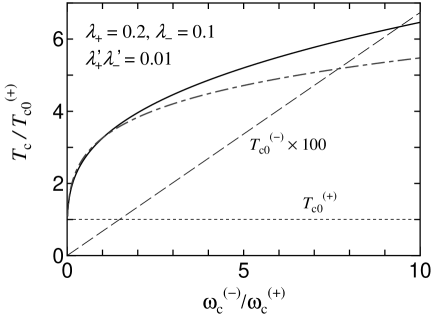
Figure 1: Transition temperatures as functions of the cutoff energy. The solid and dashed curves show ${T_{\rm c}}$ and $T_{c0}^{(-)}$, respectively. As an example, $\lambda_{+}=0.2$, $\lambda_{-}=0.1$, and $\lambda_{+}^{\prime}\lambda_{-}^{\prime}=0.01$ are assumed. The dot-dash curve shows the result when the ratio $T_{c0}^{(-)}/T_{c0}^{(+)}=0.007$ is fixed by adjusting $\lambda_{-}$.

IV Pairing Interactions

In this section, we examine the transformation of the original charge-charge and spin-spin interactions into pairing interactions between the electrons on the SFSs. We examine interactions of the form

$$H_{1}=H_{1\rm c}+H_{1z}+H_{1\perp},$$ (25)

with the charge-charge interaction (CI)

$$H_{1\rm c}=\sum_{i,j}V_{ij}^{\rm c}n_{i}n_{j},$$ (26)

the Ising-type interaction

$$H_{1z}=\sum_{i,j}J_{ij}^{z}S_{i}^{z}S_{j}^{z},$$ (27)

and the planar spin interaction

$$H_{1\perp}=\sum_{i,j}J_{ij}^{\perp}(S_{i}^{x}S_{j}^{x}+S_{i}^{y}S_{j}^{y}).$$ (28)

Here, $n_{i}=\sum_{\sigma}c_{i\sigma}^{\dagger}c_{i\sigma}$ and ${{\bm{S}}}_{i}=\frac{1}{2}\sum_{\sigma_{1}\sigma_{2}}c_{i\sigma_{1}}^{\dagger}{\bm{\sigma}}_{\sigma_{1}\sigma_{2}}c_{i\sigma_{2}}$. The CI can be derived as an effective interaction mediated by phonons and charge fluctuations, while the SI can be derived as that mediated by spin fluctuations, which includes the kinetic exchange and superexchange interactions. We have ignored the broken inversion symmetry in the interactions, although it might give rise to some interesting effects. We define $V^{z}\equiv J^{z}$ and $V^{\perp}\equiv J^{\perp}$ for simplicity of the notation. The above interactions give rise to the pairing interactions

$$\begin{array}[]{rcl}H_{1\rm c}&=&\displaystyle{\frac{1}{N}\sum_{{{\bm{k}}}{{\bm{k}}}^{\prime}\sigma\sigma^{\prime}}V_{{\rm c}}({{\bm{k}}},{{\bm{k}}}^{\prime}){\hat{\psi}}_{\sigma\sigma^{\prime}}^{\dagger}({{\bm{k}}}){\hat{\psi}}_{\sigma\sigma^{\prime}}({{\bm{k}}}^{\prime})}\\[12.0pt] H_{1z}&=&\displaystyle{\frac{1}{4N}\sum_{{{\bm{k}}}{{\bm{k}}}^{\prime}\sigma\sigma^{\prime}}\sigma\sigma^{\prime}J_{z}({{\bm{k}}},{{\bm{k}}}^{\prime}){\hat{\psi}}_{\sigma\sigma^{\prime}}^{\dagger}({{\bm{k}}}){\hat{\psi}}_{\sigma\sigma^{\prime}}({{\bm{k}}}^{\prime})}\\[12.0pt] H_{1\perp}&=&\displaystyle{-\frac{1}{2N}\sum_{{{\bm{k}}}{{\bm{k}}}^{\prime}\sigma}J_{\perp}({{\bm{k}}},{{\bm{k}}}^{\prime}){\hat{\psi}}_{\sigma-\sigma}^{\dagger}({{\bm{k}}}){\hat{\psi}}_{\sigma-\sigma}({{\bm{k}}}^{\prime})}\end{array}$$ (29)

within the BCS approximation, where we have defined

$${V^{X}_{{{\bm{q}}}}\equiv\sum_{{{\bm{R}}}_{ij}}e^{-i{{\bm{q}}}\cdot{{\bm{R}}}_{ij}}V_{ij}^{X}~{}~{}~{}\mbox{($X=c$, $z$, and $\perp$)},}$$

$V_{\rm c}({{\bm{k}}},{{\bm{k}}}^{\prime})=V_{{{\bm{k}}}-{{\bm{k}}}^{\prime}}^{\rm c}$, $V_{z}({{\bm{k}}},{{\bm{k}}}^{\prime})=V_{{{\bm{k}}}-{{\bm{k}}}^{\prime}}^{z}$, and $V_{\perp}({{\bm{k}}},{{\bm{k}}}^{\prime})=V_{{{\bm{k}}}+{{\bm{k}}}^{\prime}}^{\perp}$. The $\alpha$-components $V^{(ss^{\prime})}_{X\alpha}$ are defined by the equations analogous to eq. (18). Rewriting eq. (29) into the forms of eqs. (8) – (10), we obtain the $\alpha$-components of the singlet and triplet coupling constants

$${\begin{array}[]{rcl}V_{0\alpha}^{(ss^{\prime})}&=&\displaystyle{2V_{{\rm c}\alpha}^{(ss^{\prime})}-\frac{1}{2}J_{z\alpha}^{(ss^{\prime})}-J_{\perp\alpha}^{(ss^{\prime})}}\\[8.0pt] {\tilde{V}}_{\alpha}^{(ss^{\prime})}&=&\displaystyle{\sum_{\alpha^{\prime}{\rm(odd)}}\Bigl{[}2g_{2\alpha\alpha^{\prime}}^{(ss^{\prime})}\,V_{{\rm c}\alpha^{\prime}}^{(ss^{\prime})}+\frac{1}{2}{\bar{g}}_{2\alpha\alpha^{\prime}}^{(ss^{\prime})}J_{z\alpha^{\prime}}^{(ss^{\prime})}}\\[8.0pt] &&\displaystyle{\hskip 25.83325pt-g_{2z\alpha\alpha^{\prime}}^{(ss^{\prime})}J_{\perp\alpha^{\prime}}^{(ss^{\prime})}\Bigr{]}.}\end{array}}$$

Therefore, we obtain the transformation rule

$$\Gamma_{\alpha}^{(ss^{\prime})}=\sum_{\alpha^{\prime}X}{\cal T}_{X\alpha\alpha^{\prime}}^{(ss^{\prime})}V_{X\alpha^{\prime}}^{(ss^{\prime})},$$ (30)

where

$$\begin{array}[]{rcl}{\cal T}_{{\rm c}\alpha\alpha^{\prime}}^{(ss^{\prime})}&=&\displaystyle{2ss^{\prime}\delta_{\alpha\alpha^{\prime}}+2g_{2\alpha\alpha^{\prime}}^{(ss^{\prime})}}\\[8.0pt] {\cal T}_{{z}\alpha\alpha^{\prime}}^{(ss^{\prime})}&=&\displaystyle{-\frac{ss^{\prime}}{2}\delta_{\alpha\alpha^{\prime}}+\frac{1}{2}{\bar{g}}_{2\alpha\alpha^{\prime}}^{(ss^{\prime})}}\\[8.0pt] {\cal T}_{{\perp}\alpha\alpha^{\prime}}^{(ss^{\prime})}&=&\displaystyle{-ss^{\prime}\delta_{\alpha\alpha^{\prime}}-g_{2z\alpha\alpha^{\prime}}^{(ss^{\prime})},}\end{array}$$ (31)

and

$$\begin{array}[]{rcl}g_{2\alpha\alpha^{\prime}}^{(ss^{\prime})}&=&\displaystyle{g_{2x\alpha\alpha^{\prime}}^{(ss^{\prime})}+g_{2y\alpha\alpha^{\prime}}^{(ss^{\prime})}+g_{2z\alpha\alpha^{\prime}}^{(ss^{\prime})}}\\[8.0pt] {\bar{g}}_{2\alpha\alpha^{\prime}}^{(ss^{\prime})}&=&\displaystyle{g_{2x\alpha\alpha^{\prime}}^{(ss^{\prime})}+g_{2y\alpha\alpha^{\prime}}^{(ss^{\prime})}-g_{2z\alpha\alpha^{\prime}}^{(ss^{\prime})}}\end{array}$$ (32)

with $g_{2\nu\alpha\alpha^{\prime}}^{(ss^{\prime})}=g_{\nu\alpha\alpha^{\prime}}^{(s)}g_{\nu\alpha^{\prime}\alpha}^{(s^{\prime})}$ and

$${g_{\nu\alpha\alpha^{\prime}}^{(s)}=\frac{1}{N}\sum_{{{\bm{k}}}}\gamma_{\alpha}^{(s)}({{\bm{k}}}){\hat{g}}_{\nu}({{\bm{k}}})\bigl{[}\gamma_{\alpha^{\prime}}^{(s)}({{\bm{k}}})\bigr{]}^{*}.}$$

In particular, for the isotropic spin interaction $J_{ij}^{z}=J_{ij}^{\perp}\equiv J_{ij}$, we obtain

$$\begin{array}[]{rcl}V_{0\alpha}^{(ss^{\prime})}&=&\displaystyle{2V_{{\rm c}\alpha}^{(ss^{\prime})}-\frac{3}{2}J_{\alpha}^{(ss^{\prime})}}\\[8.0pt] {\tilde{V}}_{\alpha}^{(ss^{\prime})}&=&\displaystyle{\sum_{\alpha^{\prime}{\rm(odd)}}g_{2\alpha\alpha^{\prime}}^{(ss^{\prime})}\,\Bigl{\{}2V_{{\rm c}\alpha^{\prime}}^{(ss^{\prime})}+\frac{1}{2}J_{\alpha^{\prime}}^{(ss^{\prime})}\Bigr{\}}.}\end{array}$$ (33)

In the model with a strong on-site Coulomb interaction $U$, the interaction

$$H_{1}=\sum_{(i,j)}J\bigl{(}{{\bm{S}}}_{i}\cdot{{\bm{S}}}_{j}-\frac{1}{4}n_{i}n_{j}\bigr{)}$$ (34)

is derived in the second-order perturbation of the hopping integral $t$ with $t\ll U$. This form corresponds to the present model eq. (25) with $J_{ij}^{z}=J_{ij}^{\perp}\equiv J_{ij}$ and $V_{ij}^{{\rm c}}=-J_{ij}/4$. Therefore, from eq. (33), we obtain

$${\begin{array}[]{rcl}V_{0\alpha}^{(ss^{\prime})}&=&\displaystyle{-2J_{\alpha}^{(ss^{\prime})}}\\[4.0pt] {\tilde{V}}_{\alpha}^{(ss^{\prime})}&=&0.\end{array}}$$

Since eq. (34) does not have triplet interactions, no effect due to singlet-triplet mixing, which we will describe below, occurs.

In the above equations, $\alpha$ must be of even parity as mentioned above. Therefore, $\alpha^{\prime}$ must be of odd parity in the second terms of eq. (31), because ${\hat{{\bm{g}}}}({{\bm{k}}})$ is an odd function. The pairing interactions $V_{X\alpha^{\prime}}^{(ss^{\prime})}$ with an odd (even) $\alpha^{\prime}$ contribute to the gap function of even $\alpha$ through the triplet (singlet) components ${\tilde{V}}_{{\rm tri}}$ ($V_{{\rm sin}}$). For example, in a spherically symmetric system, a p-wave interaction contributes to both s-wave and d-wave pairings, while neither s-wave nor d-wave pairings contribute to each other.

V Two Limiting Cases

In this section, we compare the results of two opposite limiting cases: an equal-band limit and a single-band limit, which are defined below.

V.1 Equal-band limit

We define the equal-band limit by the conditions for the densities of states

$$\rho_{+}^{(\alpha)}(0)=\rho_{-}^{(\alpha)}(0)\equiv\rho_{\rm F},$$ (35)

and the interaction parameters $V_{0\alpha}^{(\pm\pm)}=V_{0\alpha}^{(\pm\mp)}\equiv V_{\alpha}^{\rm sin}$, ${\tilde{V}}_{\alpha}^{(\pm\pm)}={\tilde{V}}_{\alpha}^{(\pm\mp)}\equiv{\tilde{V}}_{\alpha}^{\rm tri}$, and $\omega_{\rm c}^{(+)}=\omega_{\rm c}^{(-)}$, which are independent of the band indexes, while the SFSs are displaced in momentum space because we have set $\langle{\tilde{\psi}}_{\pm\mp}({{\bm{k}}})\rangle=0$. We define $\lambda_{\alpha}^{\rm sin}=-\frac{1}{2}V_{\alpha}^{\rm sin}\rho_{\rm F}$ and $\lambda_{\alpha}^{\rm tri}=-\frac{1}{2}{\tilde{V}}_{\alpha}^{\rm tri}\rho_{\rm F}$. Then, we obtain ${\lambda_{\alpha}^{(ss^{\prime})}=ss^{\prime}\lambda_{\alpha}^{\rm sin}+\lambda_{\alpha}^{\rm tri},}$ i.e.,

$${\begin{array}[]{l}\lambda_{\alpha}\equiv\lambda_{+}=\lambda_{-}=\lambda_{\alpha}^{\rm sin}+\lambda_{\alpha}^{\rm tri}\\ \lambda^{\prime}_{\alpha}\equiv\lambda^{\prime}_{+}=\lambda^{\prime}_{-}=-\lambda_{\alpha}^{\rm sin}+\lambda_{\alpha}^{\rm tri}.\end{array}}$$

Setting $\omega_{\rm c}=\omega_{\rm c}^{(\pm)}$ in eq. (24), we obtain

$$\Lambda_{\alpha}=\lambda_{\alpha}\pm|\lambda^{\prime}_{\alpha}|=\left\{\begin{array}[]{c}2\lambda_{\alpha}^{\rm sin}\\ 2\lambda_{\alpha}^{\rm tri}\end{array}\right.,$$ (36)

the larger positive one of which is the physical solution. For $\Lambda_{\alpha}=2\lambda_{\alpha}^{\rm sin}$ and $2\lambda_{\alpha}^{\rm tri}$, the gap function becomes

$${\left(\begin{array}[]{c}\Delta_{\alpha}^{(+)}\\ \Delta_{\alpha}^{(-)}\end{array}\right)=\left(\begin{array}[]{c}\Delta_{\alpha}\\ -\Delta_{\alpha}\end{array}\right)~{}~{}\mbox{and}~{}~{}\left(\begin{array}[]{c}\Delta_{\alpha}\\ \Delta_{\alpha}\end{array}\right),}$$

respectively. Therefore, in this ideal case, the gap function becomes purely singlet or triplet.

V.2 Single-band limit

The single-band limit is defined so that only one of the spin-orbit split bands has a Fermi surface, which is expressed as

$$\rho_{+}^{(\alpha)}(0)=\rho_{\rm F}~{}~{}\mbox{and}~{}~{}\rho_{-}^{(\alpha)}(0)=0.$$ (37)

The limit can be used as a theoretical model for some of the Fermi surfaces in ${\rm Li_{2}Pt_{3}B}$. Since $\lambda_{-}=\lambda^{\prime}_{-}=0$ and $\Delta_{-}=0$, the linearized gap equation eq. (22) becomes $\Delta_{+}=\lambda_{+}l_{+}\Delta_{+}$. Therefore, we obtain

$$\Lambda_{\alpha}=\lambda_{\alpha}^{(++)}=\lambda_{\alpha}^{\rm sin}+\lambda_{\alpha}^{\rm tri},$$ (38)

with $\omega_{\rm c}=\omega_{\rm c}^{(+)}$. The gap function becomes

$${\left(\begin{array}[]{c}\Delta_{\alpha}^{(+)}\\ \Delta_{\alpha}^{(-)}\end{array}\right)=\left(\begin{array}[]{c}\Delta_{\alpha}\\ 0\end{array}\right).}$$

Hence, we obtain ${\cal F}_{-}({{\bm{k}}},\omega_{n})=0$ and $|\langle{\hat{d}}({{\bm{k}}})\rangle|=|\langle{\hat{d}}_{0}({{\bm{k}}})\rangle|$ from eqs. (6) and (12), where $|\cdots|$ is to eliminate arbitrary phase factors. In contrast to the equal-band limit, the amplitudes of the spin-singlet and triplet components coincide.

Thus, the properties of the superconductivity are completely different in the two limits. The disappearance of one of the SFSs causes drastic changes in the transition temperature and gap structure. This might explain the difference between the experimental results in ${\rm Li_{2}Pd_{3}B}$ and ${\rm Li_{2}Pt_{3}B}$ discussed in § 1. For example, the full-gap structure may change into a gap structure with line nodes, when the spin-orbit coupling $\alpha$ increases. We shall illustrate this in the following sections.

VI Phase Diagrams

We apply the present theory to several specific models. As an example, we suppose that the system has spherically symmetric Fermi surfaces, and ${\hat{{\bm{g}}}}({{\bm{k}}})={\hat{{\bm{k}}}}$. We set $\alpha=(l,m)$ and define the spherical harmonic functions as

$$Y_{lm}({\hat{{\bm{k}}}})=Y_{lm}(\theta_{\hat{{\bm{k}}}},\varphi_{\hat{{\bm{k}}}})=P_{l}^{m}(\cos\theta_{\hat{{\bm{k}}}})e^{im\varphi_{\hat{{\bm{k}}}}},$$

where $\theta_{\hat{{\bm{k}}}}$ and $\varphi_{\hat{{\bm{k}}}}$ denote the polar angles to express the direction of ${\hat{{\bm{k}}}}$, and $P_{l}^{m}(w)$ denotes the Legendre polynomial. The basis functions are written as

$${\gamma_{lm}^{(s)}({{\bm{k}}})=C_{lm}^{(s)}\,\theta(\omega_{\rm c}^{(s)}-|{\tilde{\xi}}_{{{\bm{k}}}s}|)\,Y_{lm}({\hat{{\bm{k}}}})}$$

with the normalization factor $C_{lm}^{(s)}$. In the expansions of the interactions, we assume that $V_{X(lm)}^{(ss^{\prime})}=V_{Xl}$ and retain the terms up to $l=2$ for simplicity. The coefficients $g_{\nu(lm)(l^{\prime}m^{\prime})}^{(ss^{\prime})}$ can be calculated straightforwardly, for example, as $g_{2z(0,0)(1,0)}^{(ss^{\prime})}=g_{2z(1,0)(0,0)}^{(ss^{\prime})}=1/3$, and so on.

In this section, we examine the two limiting cases defined in the previous section: the equal-band limit and single-band limit. The former limit is a simplified model of the system in which both SFSs exist [case (i)], while the latter limit corresponds to the system in which only one of the spin-orbit split bands has a Fermi surface [case (ii)].

VI.1 Charge-charge interaction

In the system with the CI defined by eq. (26), we obtain

$${\begin{array}[]{rcl}\Gamma_{00}^{(ss^{\prime})}&=&\displaystyle{2ss^{\prime}V_{{\rm c}0}+2V_{{\rm c}1}}\\ \Gamma_{2m}^{(ss^{\prime})}&=&\displaystyle{2ss^{\prime}V_{{\rm c}2}+\frac{4}{5}V_{{\rm c}1}}\end{array}}$$

with $m=\pm 2,\pm 1,0$. Therefore, in the equal-band limit, we obtain

$$\begin{array}[]{rclrcl}\lambda_{00}&=&\displaystyle{\lambda_{{\rm c}0}+\lambda_{{\rm c}1},{}}&~{}\lambda^{\prime}_{00}&=&\displaystyle{-\lambda_{{\rm c}0}+\lambda_{{\rm c}1},}\\ \lambda_{2m}&=&{\lambda_{{\rm c}2}+\frac{2}{5}\lambda_{{\rm c}1},{}}&~{}\lambda_{2m}^{\prime}&=&{-\lambda_{{\rm c}2}+\frac{2}{5}\lambda_{{\rm c}1},}\end{array}$$ (39)

with $\lambda_{{\rm c}l}=-V_{{\rm c}l}\rho_{\rm F}$. Similar results, except the terms including $\lambda_{{\rm c}2}$, have been obtained by Samokhin and Mineev Sam08 . The gap function of the s-wave state has a full-gap structure, while those of the d-wave states have line nodes. In the present isotropic model, the transition temperatures of the d-wave pairing are degenerate with respect to $m$, and a d-wave state expressed by the linear combination of those degenerate states occurs below ${T_{\rm c}}$. By minimizing the free energy, we obtain a d-wave state with a full-gap structure, but this is an artifact due to the isotropy of the model. By taking into account the anisotropy that exists in real crystal systems, the degeneracy is lifted, and some of the solutions with different $m$’s show the highest ${T_{\rm c}}$. Therefore, considering the reality, we ought to regard the d-wave states as line-node states at least near the transition temperature, while at low temperatures the order parameters with different $m$’s can be mixed and the full-gap state may occur. From eqs. (36) and (39), we obtain

$$\begin{array}[]{rcl}\Lambda_{0}&=&\max(2\lambda_{{\rm c}0},2\lambda_{{\rm 1}},0)\\ \Lambda_{2}&=&\max(2\lambda_{{\rm c}2},4\lambda_{{\rm 1}}/5,0).\end{array}$$ (40)

Hence, the resultant coupling constant is expressed as

$$\Lambda=\max(2\lambda_{{\rm c}0},2\lambda_{{\rm c}2},2\lambda_{{\rm c}1},0),$$ (41)

which gives the phase diagram shown in Fig. 2. The phase diagrams in this paper are not those at $T=0$, but the diagrams of the phases that give ${T_{\rm c}}$. Successive transitions to other superconducting phases may occur below ${T_{\rm c}}$.

It is found from eqs. (40) and (41) that, when the even-parity pairing is induced by the spin-triplet pairing, it will have the s-wave symmetry rather than the d-wave symmetry, because $2\lambda_{{\rm c}1}>4\lambda_{{\rm c}1}/5$ for $\lambda_{{\rm c}1}>0$. Although the p-wave attractive interaction contributes to both the s-wave pairing and the d-wave pairing, the contribution to the s-wave pairing is larger by a factor of $5/2$. Consequently, as shown in Fig. 2, when the s-wave and d-wave pairing interactions $\lambda_{{\rm c}0}$ and $\lambda_{{\rm c}2}$ are weak or repulsive, the p-wave pairing interaction induces the s-wave superconductivity. Such an s-wave state has a full-gap structure similarly to the conventional s-wave state, but is at the same time a purely spin-triplet state that has the d-vector $\langle{\hat{{\bm{d}}}}({{\bm{k}}})\rangle=\langle{\hat{d}}({{\bm{k}}})\rangle{\hat{{\bm{g}}}}({{\bm{k}}})$ with an even parity amplitude $\langle{\hat{d}}({{\bm{k}}})\rangle$. The gap function becomes $\Delta_{{{\bm{k}}}s}=-2V_{{\rm c}1}s_{{{\bm{k}}}}\langle{\hat{d}}({{\bm{k}}})\rangle\propto s_{{{\bm{k}}}}\theta(\omega_{\rm c}^{(s)}-|\xi_{{{\bm{k}}}}^{(s)}|)$, which does not have nodes on the Fermi surface but has the phase factor $s_{{{\bm{k}}}}$. The energy gaps of the quasi-particle energies $E_{{{\bm{k}}}\pm}$ become constants $|\Delta_{(0,0)}^{\pm}|$ independent of ${\hat{{\bm{k}}}}$, from eqs. (13) and (20). The s-wave spin-triplet order is suggested in ${\rm Li_{2}Pt_{3}B}$ by Yuan et al. Yua06 , although ${\rm Li_{2}Pt_{3}B}$ is in the opposite limit. Interestingly, however strong the repulsive spin-singlet interaction is, a weaker attractive spin-triplet interaction could cause the s-wave superconductivity mentioned above, owing to the cancellation effect between the intra- and inter-band interactions. On the other hand, in Fig. 2, the d-wave phase in the upper area and the s-wave phase in the right area are conventional pure spin-singlet phases induced by d-wave and s-wave pairing interactions, respectively. Away from the equal-band limit, the mixing of spin-singlet and triplet states occurs.

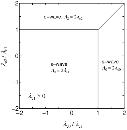
Figure 2: Phase diagram of the system with the CI, when both of the SFSs exist. The spin-triplet interaction is assumed to be attractive.

In the single band limit, the effective coupling constant becomes

$$\Lambda=\max(\Lambda_{0},\Lambda_{2},0),$$ (42)

where $\Lambda_{0}=\lambda_{{\rm c}0}+\lambda_{{\rm c}1}$ and $\Lambda_{2}=\lambda_{2m}=\lambda_{{\rm c}2}+\frac{2}{5}\lambda_{{\rm c}1}$, which gives the phase diagram shown in Fig. 3. In both the d-wave and s-wave phases, the singlet-triplet mixing occurs. It is found that the p-wave spin-triplet pairing interaction stabilizes both the d-wave and s-wave phases, but in contrast to the equal band limit, the superconductivity is suppressed, where both of the d-wave and s-wave interactions are repulsive and sufficiently strong.

Figure 3: Phase diagram of the system with the CI, when only one of the spin-orbit split bands has a Fermi surface. The spin-triplet interaction is assumed to be attractive.

Figure 4 shows the transitions when one of the SFSs disappears. In the gray area, the s-wave full-gap state changes into the d-wave state. Since the d-wave state can be regarded as a line-node state as argued above, the transition in this area is a type of FLT. This result may explain the observations in ${\rm Li_{2}Pd_{3}B}$ and ${\rm Li_{2}Pt_{3}B}$, as discussed in § I. In this case, the initial state of the transition is the s-wave spin-triplet state, and the final state is the d-wave state with both spin-singlet and triplet components. The conventional s-wave spin-singlet state cannot be the initial state that changes into the final d-wave state, as shown in Fig. 4. This result is roughly interpreted as follows. For the d-wave state to occur as the final state in the single-band limit, the s-wave interaction needs to be weak or repulsive. Therefore, if the s-wave state occurs as the initial state for the same coupling constants, it must be a spin-triplet state induced by the p-wave interaction, rather than a spin-singlet state induced by the s-wave interaction. This interpretation is not a rigorous proof, but is verified by eqs. (41) and (42) and Fig. 4. In most of the gray area, the s-wave interaction is repulsive ($\lambda_{{\rm c}0}<0$), while the p-wave and d-wave interactions are attractive; the former is stronger than the latter ($0<\lambda_{{\rm c}2}<\lambda_{{\rm c}1}$). These conditions are likely to be satisfied in real materials in which both the screened short-range Coulomb repulsion and phonon-mediated pairing interactions are strong.

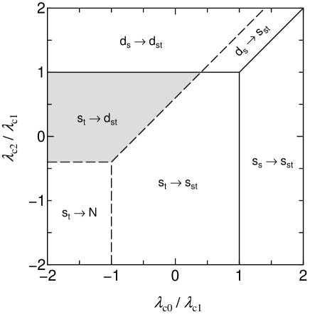
Figure 4: Superposition of the phase diagrams in Figs. 2 and 3 to show the transition when one of the SFSs disappears owing to the increase in the spin-orbit coupling. The spin-triplet interaction is assumed to be attractive ($\lambda_{{\rm c}1}>0$). The notation “${\rm a}\rightarrow{\rm b}$” means the transition from phase “${\rm a}$” to phase “${\rm b}$”, where d, s, and N mean the d- and s-wave superconducting phases and the normal phase, respectively. The suffixes s, t, and st mean the spin-singlet, triplet, and singlet-triplet mixed states, respectively. For example, “${\rm s}_{\rm t}\rightarrow{\rm d}_{\rm st}$” means the transition from the s-wave spin-triplet state to the d-wave state with both spin-singlet and triplet components.

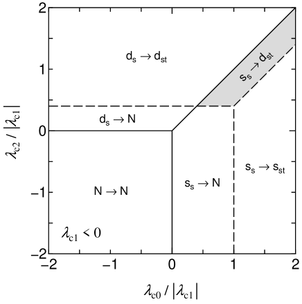
Figure 5: Transitions when the interaction is of the charge-charge type and the p-wave component is repulsive. The legends are the same as those in Fig. 4.

Figure 5 shows the transitions in the case that the p-wave component of the interaction is repulsive, which might be unlikely if we suppose a phonon-mediated pairing interaction as the CI Fou77 . In the gray area, the s-wave full-gap state changes into the d-wave state. In contrast to the previous case, the initial s-wave state is of spin-singlet pairing.

VI.2 Spin-spin interactions

Next, we examine the phase diagrams and the transitions of the systems with the SIs $H_{z1}$ and $H_{\perp 1}$ of eqs. (27) and (28). In this type of interaction, anisotropies of interactions in the spin space play an essential role. Depending on the anisotropy and the sign of the interactions, the transition from the full-gap state to the line-node state (FLT) can occur.

VI.2.1 Ising-type interaction

In the system with only the Ising-type interaction eq. (27), we obtain

$${\begin{array}[]{rcl}\Gamma_{00}^{(ss^{\prime})}&=&{-\frac{1}{2}ss^{\prime}J_{z0}+\frac{1}{6}J_{z1}}\\[4.0pt] \Gamma_{20}^{(ss^{\prime})}&=&{-\frac{1}{2}ss^{\prime}J_{z2}-\frac{1}{15}J_{z1}}\\[4.0pt] \Gamma_{2,\pm 1}^{(ss^{\prime})}&=&{-\frac{1}{2}ss^{\prime}J_{z2}}\\[4.0pt] \Gamma_{2,\pm 2}^{(ss^{\prime})}&=&{-\frac{1}{2}ss^{\prime}J_{z2}+\frac{1}{5}J_{z1}}.\end{array}}$$

(i) In the equal-band limit, we obtain

$$\begin{array}[]{rclrcl}\lambda_{00}&=&{\lambda_{z0}-\frac{1}{3}\lambda_{z1},{}}&~{}\lambda_{00}^{\prime}&=&{-\lambda_{z0}-\frac{1}{3}\lambda_{z1},}\\[4.0pt] \lambda_{20}&=&{\lambda_{z2}+\frac{2}{15}\lambda_{z1},{}}&~{}\lambda_{20}^{\prime}&=&{-\lambda_{z2}+\frac{2}{15}\lambda_{z1},}\\[4.0pt] \lambda_{2\pm 1}&=&{\lambda_{z2},{}}&~{}\lambda_{2\pm 1}^{\prime}&=&{-\lambda_{z2},}\\[4.0pt] \lambda_{2\pm 2}&=&{\lambda_{z2}-\frac{4}{5}\lambda_{z1},{}}&~{}\lambda_{2\pm 2}^{\prime}&=&{-\lambda_{z2}-\frac{4}{5}\lambda_{z1},}\\ \end{array}$$ (43)

with $\lambda_{zl}=\frac{1}{4}J_{zl}\rho_{\rm F}$. Hence, we obtain

$$\begin{array}[]{rcl}\Lambda_{0}&=&\max(2\lambda_{z0},-\frac{2}{3}\lambda_{z1},0),\\[4.0pt] \Lambda_{20}&=&\max(2\lambda_{z2},\frac{4}{15}\lambda_{z1},0),\\[4.0pt] \Lambda_{2,\pm 1}&=&\max(2\lambda_{z2},0),\\[4.0pt] \Lambda_{2,\pm 2}&=&\max(2\lambda_{z2},-\frac{8}{5}\lambda_{z1},0),\end{array}$$ (44)

and

$$\Lambda=\max(2\lambda_{z0},2\lambda_{z2},-\frac{8}{5}\lambda_{z1},\frac{4}{15}\lambda_{z1},0).$$ (45)

Interestingly, the repulsive p-wave spin-triplet interaction stabilizes both the d-wave spin-triplet state with $(l,m)=(2,\pm 2)$ and the s-wave spin-triplet state. However, because of the numerical factors in front of $\lambda_{z1}$, the former overcomes the latter. (ii) In the single-band limit, we obtain

$$\begin{array}[]{rcl}\Lambda_{0}&=&{\lambda_{z0}-\frac{1}{3}\lambda_{z1},}\\[4.0pt] \Lambda_{20}&=&{\lambda_{z2}+\frac{2}{15}\lambda_{z1},}\\[4.0pt] \Lambda_{2,\pm 1}&=&{\lambda_{z2},}\\[4.0pt] \Lambda_{2,\pm 2}&=&{\lambda_{z2}-\frac{4}{5}\lambda_{z1}}.\end{array}$$ (46)

The resultant coupling constant is

$$\Lambda=\max(\Lambda_{0},\Lambda_{20},\Lambda_{2,\pm 1},\Lambda_{2,\pm 2},0).$$ (47)

VI.2.2 Planar spin interaction

In the system with only the planar spin interaction eq. (28), we obtain

$${\begin{array}[]{rcl}\Gamma_{00}^{(ss^{\prime})}&=&{-ss^{\prime}J_{\perp 0}+\frac{1}{3}J_{\perp 1},}\\[4.0pt] \Gamma_{20}^{(ss^{\prime})}&=&{-ss^{\prime}J_{\perp 2}+\frac{4}{15}J_{\perp 1},}\\[4.0pt] \Gamma_{2,\pm 1}^{(ss^{\prime})}&=&{-ss^{\prime}J_{\perp 2}+\frac{1}{5}J_{\perp 1},}\\[4.0pt] \Gamma_{2,\pm 2}^{(ss^{\prime})}&=&{-ss^{\prime}J_{\perp 2}}.\end{array}}$$

(i) In the equal-band limit, we obtain

$${\begin{array}[]{rclrcl}\lambda_{00}&=&{\lambda_{\perp 0}-\frac{1}{3}\lambda_{\perp 1},{}}&~{}\lambda_{00}^{\prime}&=&{-\lambda_{\perp 0}-\frac{1}{3}\lambda_{\perp 1},}\\[4.0pt] \lambda_{20}&=&{\lambda_{\perp 2}-\frac{4}{15}\lambda_{\perp 1},{}}&~{}\lambda_{20}^{\prime}&=&{-\lambda_{\perp 2}-\frac{4}{15}\lambda_{\perp 1},}\\[4.0pt] \lambda_{2\pm 1}&=&{\lambda_{\perp 2}-\frac{1}{5}\lambda_{\perp 1},{}}&~{}\lambda_{2\pm 1}^{\prime}&=&{-\lambda_{\perp 2}-\frac{1}{5}\lambda_{\perp 1},}\\[4.0pt] \lambda_{2\pm 2}&=&{\lambda_{\perp 2},{}}&~{}\lambda_{2\pm 2}^{\prime}&=&{-\lambda_{\perp 2},}\end{array}}$$

with $\lambda_{\perp l}=\frac{1}{2}J_{\perp l}\rho_{\rm F}$. Hence, we obtain

$${\begin{array}[]{rcl}\Lambda_{0}&=&\max(2\lambda_{\perp 0},-\frac{2}{3}\lambda_{\perp 1},0),\\[4.0pt] \Lambda_{20}&=&\max(2\lambda_{\perp 2},-\frac{8}{15}\lambda_{\perp 1},0),\\[4.0pt] \Lambda_{2,\pm 1}&=&\max(2\lambda_{\perp 2},-\frac{2}{5}\lambda_{\perp 1},0),\\[4.0pt] \Lambda_{2,\pm 2}&=&\max(2\lambda_{\perp 2},0),\end{array}}$$

and

$${\Lambda=\max(2\lambda_{\perp 0},2\lambda_{\perp 2},-\frac{2}{3}\lambda_{\perp 1},0).}$$

(ii) In the single-band limit, we obtain

$${\begin{array}[]{rcl}\Lambda_{0}&=&{\lambda_{\perp 0}-\frac{1}{3}\lambda_{\perp 1},}\\[4.0pt] \Lambda_{20}&=&{\lambda_{\perp 2}-\frac{4}{15}\lambda_{\perp 1},}\\[4.0pt] \Lambda_{2,\pm 1}&=&{\lambda_{\perp 2}-\frac{1}{5}\lambda_{\perp 1},}\\[4.0pt] \Lambda_{2,\pm 2}&=&{\lambda_{\perp 2}}.\end{array}}$$

The resultant coupling constant is the maximum positive one, as given by eq. (47).

VI.2.3 Isotropic spin interaction

Lastly, in the system with the isotropic spin interaction $J_{ij}^{z}=J_{ij}^{\perp}\equiv J_{ij}$, we obtain

$${\begin{array}[]{rcl}\Gamma_{0}^{(ss^{\prime})}&=&{-ss^{\prime}\frac{3}{2}J_{0}+\frac{1}{2}J_{1},}\\[4.0pt] \Gamma_{2}^{(ss^{\prime})}&=&{-ss^{\prime}\frac{3}{2}J_{2}+\frac{1}{5}J_{1}.}\end{array}}$$

(i) In the equal-band limit, we obtain

$${\begin{array}[]{rclrcl}\lambda_{0}&=&{\lambda_{0}-\frac{1}{3}\lambda_{1},{}}&~{}\lambda_{0}^{\prime}&=&{-\lambda_{0}-\frac{1}{3}\lambda_{1},}\\[4.0pt] \lambda_{2}&=&{\lambda_{2}-\frac{2}{15}\lambda_{1},{}}&~{}\lambda_{2}^{\prime}&=&{-\lambda_{2}-\frac{2}{15}\lambda_{1}.}\end{array}}$$

with $\lambda_{l}=\frac{3}{4}J_{l}\rho_{\rm F}$. Hence, we obtain

$${\begin{array}[]{rcl}\Lambda_{0}&=&\max(2\lambda_{0},-\frac{2}{3}\lambda_{1},0),\\[4.0pt] \Lambda_{2}&=&\max(2\lambda_{2},-\frac{4}{15}\lambda_{1},0),\end{array}}$$

and

$$\Lambda=\max(2\lambda_{0},2\lambda_{2},-\frac{2}{3}\lambda_{1},0).$$ (48)

(ii) In the single-band limit, we obtain

$${\begin{array}[]{rcl}\Lambda_{0}&=&{\lambda_{0}-\frac{1}{3}\lambda_{1},}\\[4.0pt] \Lambda_{2}&=&{\lambda_{2}-\frac{2}{15}\lambda_{1},}\end{array}}$$

and

$$\Lambda=\max(\lambda_{0}-\frac{1}{3}\lambda_{1},\lambda_{2}-\frac{2}{15}\lambda_{1},0).$$ (49)

VI.2.4 Phase diagrams and transitions

In this subsection, we examine the phase diagrams of the systems with SIs. Figures 6 - 11 show the phase diagrams of the systems with various types of SIs (see Table 1). In each figure, two phase diagrams are superposed as shown in Figs. 2 - 4 for the CI. The solid lines show the phase boundaries in case (i), and the broken lines and the texts in brackets show the phase boundaries and the symmetries of the phases in case (ii), respectively. As explained in the caption of Fig. 4, the notation “${\rm a}\rightarrow{\rm b}$” means the transition from phase “a” to phase “b”, when one of the SFSs disappears [case (i) $\rightarrow$ case (ii)]. In addition to the characters “s”, “d”, and “N”, we have defined the notation “2$m$” that means the d-wave state with $\Delta\propto Y_{2m}$.

In case (i), anomalous even-parity (s- and d-wave) spin-triplet superconducting phases occur, where both the s- and d-wave components of the interactions are repulsive. Ising-type interactions induce d-wave spin-triplet states with different $m$’s for either sign of the p-wave component (Figs. 6 and  7), in contrast to the CI. The magnetically mediated pairing interactions could also induce s-wave spin-triplet states, when the interaction is planar or isotropic and their p-wave component is repulsive (Figs. 8 - 11). These results are quite different from that for the system with the CI, in which an s-wave spin-triplet state occurs only when the p-wave component of the interaction is attractive. These differences are explained as follows. When singlet interactions are repulsive, only a triplet p-wave interaction contributes to the even-parity state through the mixing effect due to spin-orbit coupling. Depending on the sign of the second terms of the matrix elements ${\cal T}_{X\alpha\alpha^{\prime}}^{(ss^{\prime})}$ ($X={\rm c},z,\perp$) defined by eq. (31), an attractive or repulsive p-wave interaction may contribute to the superconductivity of the anomalous type. Independently of the type of the interactions, such an anomalous phase disappears, when one of the SFSs disappears owing to the stronger spin-orbit coupling.

Figure 6: Phase diagrams and transitions for Ising-type interaction with attractive p-wave components. Solid and broken lines are the phase boundaries in cases (i) and (ii), respectively. The states in the latter case are shown in the brackets. The notation “2$m$” means the d-wave state with the quantum number $(2,m)$ (see the text). The other legends are as shown in the caption of Fig. 4.

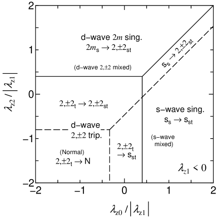
Figure 7: Phase diagrams and transitions for Ising-type interaction with repulsive p-wave components. The legends are as shown in the captions of Figs. 4 and 6.

Figure 8: Phase diagrams and transitions for planar spin interaction with attractive p-wave components. The legends are as shown in the captions of Figs. 4 and 6.

Figure 9: Phase diagrams and transitions for planar spin interaction with repulsive p-wave components. The legends are as shown in the captions of Figs. 4 and 6.

Figure 10: Phase diagrams and transitions for isotropic spin interaction with attractive p-wave components. The legends are as shown in the captions of Figs. 4 and 6.

Figure 11: Phase diagrams and transitions for isotropic spin interaction with repulsive p-wave components. The legends are as shown in the captions of Figs. 4 and 6.

Table 1: Table of the phase diagrams.

Type of coupling p-wave component interaction constant $\lambda_{1}>0$ $\lambda_{1}<0$ Ising $J_{z}\neq 0$, $J_{\perp}=0$ Fig. 6 Fig. 7 Planar $J_{z}=0$, $J_{\perp}\neq 0$ Fig. 8 Fig. 9 Isotropic $J_{z}=J_{\perp}\equiv J$ Fig. 10 Fig. 11

VI.2.5 Transitions from the full-gap state to the line-node state

The FLT due to the disappearance of one of the SFSs also occurs for the SI, as shown in Figs. 6 - 11, which are summarized in Table 2. Practically, we can regard d-wave states as line-node states, even when they degenerate with respect to $m$, by the argument in § VI.1.

Table 2: Relation between the type of interaction and the signs of the coupling constants for the FLT to occur. In each phase diagram, the signs are those for the major part of the area in which the FLT occurs. The double sign $\pm$ means that $\lambda_{2}$ can take either sign, but the absolute value is small. “${\rm s_{s}}$” and “${\rm s_{t}}$” denote the s-wave spin-singlet and triplet states, respectively.

Type of Sign of $\lambda_{l}$ FLT Phase interaction  s  p  d ${\rm s}\rightarrow{\rm d}\,(l,m)$ diagram Charge $-$ $+$ $+$ ${\rm s_{t}}\rightarrow{\rm d}\,(2,m)$ Fig. 4 $+$ $-$ $+$ ${\rm s_{s}}\rightarrow{\rm d}\,(2,m)$ Fig. 5 Ising spin $+$ $+$ $+$ ${\rm s_{s}}\rightarrow{\rm d}\,(2,0)$ Fig. 6 $+$ $-$ $+$ ​​ ${\rm s_{s}}\rightarrow{\rm d}\,(2,\pm 2)$ ​​ Fig. 7 Planar spin $+$ $+$ $+$ ​​ ${\rm s_{s}}\rightarrow{\rm d}\,(2,\pm 2)$ ​​ Fig. 8 $-$ $-$ $\pm$ ${\rm s_{t}}\rightarrow{\rm d}\,(2,0)$ Fig. 9 Isotropic spin $+$ $+$ $+$ ${\rm s_{s}}\rightarrow{\rm d}\,(2,m)$ Fig. 10 $-$ $-$ $\pm$ ${\rm s_{t}}\rightarrow{\rm d}\,(2,m)$ Fig. 11

In these phase diagrams, the regions where the FLT occurs are narrower than that in the phase diagram (Fig. 4) for the CI. Furthermore, it seems difficult that the s-wave component becomes attractive for interactions of magnetic origin. If we exclude such a situation, the remaining possibilities are planar and isotropic spin interactions with $\lambda_{1}<0$. However, in such cases, the FLT occurs only in small regions, in which the pairing interaction is very weak. Therefore, in the present theory, if the FLT occurs, it is most likely that the CI is the most dominant pairing interaction.

VII Summary and Discussion

We have examined the superconductivity in noncentrosymmetric systems with various types of interactions between electrons. We have presented a formulation of the superconductivity, and obtained the transition temperatures and gap functions, including the results that have been obtained by previous authors Gor01 ; Ser04 ; Fri04 ; Sam08 . We have derived the pairing interaction eq. (30) between the two electrons on the SFSs from interactions between original electrons. The transformation matrices ${\cal T}_{X\alpha\alpha^{\prime}}^{(ss^{\prime})}$ for three types of interactions, i.e., $V_{ij}^{{\rm c}}$, $J_{ij}^{z}$, and $J_{ij}^{\perp}$, are obtained. We have examined two kinds of order-parameter mixing effects in such superconductors due to the strong spin-orbit coupling: One is the parity mixing of the spin-singlet pairs $\langle{\hat{d}}_{0}({{\bm{k}}})\rangle$ and the triplet pairs $\langle{\hat{d}}({{\bm{k}}})\rangle$, and the other is the interband mixing of the pairs on different SFSs, i.e., $\langle{\tilde{\psi}}_{++}({{\bm{k}}})\rangle$ and $\langle{\tilde{\psi}}_{--}({{\bm{k}}})\rangle$, due to interband pair hopping.

First, we have examined the equal-band limit, where $\lambda_{s}$, $\lambda^{\prime}_{s}$, and $\omega_{\rm c}^{(s)}$ do not depend on the band index $s=\pm$. Note that this limit does not imply the absence of spin-orbit coupling, because the split of the Fermi surfaces is taken into account by setting $\langle{\tilde{\psi}}_{\pm\mp}({{\bm{k}}})\rangle=0$. In this limit, since the parity mixing effect is suppressed, a pure spin-singlet state or a pure spin-triplet state occurs, while the interband mixing effect becomes most efficient. Second, we have examined the single-band limit, where $\rho_{-}(0)=0$. In this limit, the amplitudes of the spin-singlet and triplet components coincide, in contrast to the equal-band limit. When one of the SFSs disappears, the interband mixing effect disappears, while the singlet-triplet mixing effect becomes most efficient. Between these two limits, the drastic changes explained below take place.

It is found that interband interactions could enhance the superconducting transition temperature ${T_{\rm c}}$ markedly, even if they are very small, as demonstrated in Fig. 1. For example, when $\lambda_{+}=0.2$, $\lambda_{-}=0.1$, and $\omega_{c}^{(-)}/\omega_{c}^{(+)}=2$, the ${T_{\rm c}}$’s of independent bands ($\lambda^{\prime}_{+}=\lambda^{\prime}_{-}=0$) are estimated as $T_{c0}^{(+)}/1.13\omega_{\rm c}^{(+)}\approx 0.00764$ and $T_{c0}^{(-)}\approx 0.0135\times T_{c0}^{(+)}\ll T_{c0}^{(+)}$. In this case, small interband interactions, such as $\lambda^{\prime}_{+}=\lambda^{\prime}_{-}=0.1$, enhance the transition temperature up to ${T_{\rm c}}\approx 3.96\times T_{c0}^{(+)}\gg T_{c0}^{(+)}$.

This effect may partly explain the large difference between the ${T_{\rm c}}$’s observed in ${\rm Li_{2}Pd_{3}B}$ and ${\rm Li_{2}Pt_{3}B}$ (7 and 2.7 K, respectively). In the latter compound, some of the Fermi surfaces lose their partners owing to the stronger spin-orbit coupling Shis11 , and they do not benefit from the interband mixing effect. This explanation is the case if Fermi surfaces without partners dominate the superconductivity in the latter compound. Their contributions to the density of states are large, according to the first-principles calculation by Shishidou and Oguchi Shis11 .

In addition, we have examined the effect of the difference between the two effective cutoff energies $\omega_{c}^{(+)}$ and $\omega_{c}^{(-)}$. The difference can be large in interactions mediated by spin and charge fluctuations, because each pair of Fermi surfaces has a different nesting condition, which is sensitive to the shape of the Fermi surfaces. It is found that the transition temperature strongly depends on the ratio $\omega_{c}^{(-)}/\omega_{c}^{(+)}$ as shown in Fig. 1.

Next, we have examined models with spherically symmetric Fermi surfaces and ${\hat{{\bm{g}}}}({{\bm{k}}})={\hat{{\bm{k}}}}$ as an example. The resultant phase diagrams drastically change when one of the SFSs disappears. In particular, we have derived areas where the transition from the full-gap state to the line-node state (FLT) occurs. The FLT occurs in many cases; however, analyzing the phase diagrams, it is found that it occurs in a wider realistic parameter region for the CI, while in rather narrower unrealistic parameter regions for the SIs. Therefore, the CI would be the dominant pairing interaction in many of the systems in which the FLT is observed. When the s-wave interaction is strongly repulsive, for example, owing to the strong on-site (screened) Coulomb repulsion, and the p-wave and d-wave interactions are attractive, we obtain a large region where the FLT occurs (see Fig. 4).

Therefore, the inexistence of the partners in some of the SFSs in ${\rm Li_{2}Pt_{3}B}$, which has been found by Shishidou and Oguchi Shis11 , may play an essential role in the differences of the superconductivity in ${\rm Li_{2}Pt_{3}B}$ from that in ${\rm Li_{2}Pd_{3}B}$. If the FLT occurs and the present scenario is the case in these compounds, it is most likely that the full-gap state in ${\rm Li_{2}Pd_{3}B}$ and the line-node state in ${\rm Li_{2}Pt_{3}B}$ are an s-wave nearly spin-triplet state and a d-wave state that has both spin-singlet and triplet components of comparable weights, respectively, which are induced by the CI. On the other hand, if the full-gap state also occurs in ${\rm Li_{2}Pt_{3}B}$ Haf09 , both states are of s-wave pairing, which are a nearly spin-singlet state in ${\rm Li_{2}Pd_{3}B}$ and a singlet-triplet mixed state of comparable weights in ${\rm Li_{2}Pt_{3}B}$.

Table 3: Anomalous spin-triplet states and properties of interactions. The signs are those for the major parts of the areas in which anomalous spin-triplet states occur. See corresponding phase diagrams. The $+$ sign means that the interaction is attractive between original electrons.

Type of Sign of $\lambda_{l}$ Anomalous interaction  s  p  d   triplet state Charge $\pm$ $+$ $\pm$ s-wave Ising spin $-$ $+$ $-$ d-wave, $Y_{20}$ $-$ $-$ $-$ d-wave, $Y_{2,\pm 2}$ Planar spin $-$ $-$ $-$ s-wave Isotropic spin $-$ $-$ $-$ s-wave

It is found that the magnetically mediated pairing interaction can induce the d-wave spin-triplet states as well as the s-wave spin-triplet state. We summarize the relation between the anomalous spin-triplet states and the properties of the interaction in Table 3. The magnetic anisotropy of the Ising-type interaction plays an essential role in the occurrence of the d-wave spin-triplet states, as summarized in Table 3. The terms $2\lambda_{z1}/15$ in $\lambda_{20}$ and $\lambda^{\prime}_{20}$ and the terms $-4\lambda_{z1}/5$ in $\lambda_{2,\pm 2}$ and $\lambda^{\prime}_{2,\pm 2}$ in eq. (43) induce the d-wave spin-triplet states, when $\lambda_{z1}>0$ and $\lambda_{z1}<0$, respectively. Furthermore, when the spin-spin interaction is planar or isotropic, a repulsive p-wave interaction can induce the s-wave spin-triplet state, if the even-parity interactions are repulsive or weak.

Lastly, we discuss the experimental result of the Knight shift in ${\rm Li_{2}Pt_{3}B}$ Nis07 , which exhibits a flat temperature dependence. As we mentioned in § I, it seems that conventional theory could not explain this result. If we assume that the spin susceptibility remains unchanged across ${T_{\rm c}}$, we obtain $\langle{\hat{d}}_{z}({{\bm{k}}})\rangle=\langle{\hat{d}}_{0}({{\bm{k}}})\rangle=0$ for the majority of ${{\bm{k}}}$’s. Since $\langle{\hat{d}}_{z}({{\bm{k}}})\rangle=\langle{\hat{d}}({{\bm{k}}})\rangle{\hat{g}}_{z}({{\bm{k}}})$, we obtain $\langle{\hat{d}}({{\bm{k}}})\rangle=0$ or ${\hat{g}}_{z}({{\bm{k}}})=\cos{\bar{\theta}}_{{{\bm{k}}}}=0$. Therefore, this leads to a contradiction that all the superconducting gap functions vanish as $\langle{\hat{{\bm{d}}}}({{\bm{k}}})\rangle=\langle{\hat{d}}({{\bm{k}}})\rangle\,{\hat{{\bm{g}}}}({{\bm{k}}})={{\bm{0}}}$ and $\langle d_{0}({{\bm{k}}})\rangle=0$, unless the superconductivity occurs mainly on parts of Fermi surfaces in which ${\bar{\theta}}_{{{\bm{k}}}}=\pi/2$ is satisfied. However, in ${\rm Li_{2}Pt_{3}B}$, since the sample was powder, the angles between the magnetic field and the crystal axes would have distributed randomly. One of the possible explanations for this is that the states of the sample, such as the gap function of the superconductivity and the orientations of the powders, are considerably affected by the magnetic field applied in the measurement. A theoretical interpretation of the behavior of the Knight shift remains for future studies.

In conclusion, the superconductivity in noncentrosymmetric system drastically changes when one of the SFSs vanishes as the spin-orbit coupling increases. For example, the gap structures, transition temperatures, and phase diagrams are quite different depending on whether both SFSs exist. In particular, under some conditions, the FLT occurs when one of the SFSs disappears. The area of the FLT in the phase diagram is largest when the pairing interaction is the CI and the condition $\lambda_{{\rm c}1}>\lambda_{{\rm c}2}>0>\lambda_{{\rm c}0}$ is satisfied. The latter condition seems realistic in real materials if we assume the CI. Therefore, within the present theory, it is most likely that the CI is the dominant pairing interaction in systems in which an FLT occurs, although possibilities of magnetically induced pairing interactions are not excluded. Anomalous superconducting states, such as the s-wave and d-wave spin-triplet states, are induced by an attractive or repulsive p-wave spin-triplet interaction in the presence of interband spin-triplet-pair hopping interactions, which are active only when both SFSs exist. These behaviors are sensitive to the type of pairing interaction.

ACKNOWLEDGMENTS

We wish to thank T. Shishidou for useful discussions and information on their results of the first-principles calculation in ${\rm Li_{2}Pd_{3}B}$ and ${\rm Li_{2}Pt_{3}B}$. We are very grateful to H. Tou for useful discussions and information on practice and analysis in NMR experiments.

References

(1) L. P. Gor’kov and E. I. Rashba:
Phys. Rev. Lett. 87 (2001) 037004.
(2) I. A. Sergienko and S. H. Curnoe:
Phys. Rev. B 70 (2004) 214510.
(3)
P. A. Frigeri, D. F. Agterberg, A. Koga, and M. Sigrist:
Phys. Rev. Lett. 92 (2004) 097001.
(4) N. Hayashi, K. Wakabayashi, P. A. Frigeri, and M. Sigrist:
Phys. Rev. B 73 (2006) 024504; (2006) 092508.
(5) S. Fujimoto: Phys. Rev. B 72 (2005) 024515.
(6) For a review, see
S. Fujimoto: J. Phys. Soc. Jpn. 76 (2007) 051008,
and references therein.
(7) Y. Yanase and M. Sigrist:
J. Phys. Soc. Jpn. 76 (2007) 043712.
(8) K. V. Samokhin and V. P. Mineev:
Phys. Rev. B 77 (2008) 104520.
(9) C.-K. Lu and S. Yip:
Phys. Rev. B 77 (2008) 054515.
(10)
T. Shishidou and T. Oguchi: submitted to Phys. Rev. Lett.
(11)
K. Togano, P. Badica, Y. Nakamori, S. Orimo, H. Takeya,
and K. Hirata: Phys. Rev. Lett. 93 (2004) 247004.
(12)
P. Badica, T. Kondo, and K. Togano:
J. Phys. Soc. Jpn. 74 (2005) 1014.
(13)
M. Nishiyama, Y. Inada, and G.-Q. Zheng:
Phys. Rev. B 71 (2005) 220505(R).
(14)
M. Nishiyama, Y. Inada, and G.-Q. Zheng:
Phys. Rev. Lett. 98 (2007) 047002.
(15)
H. Q. Yuan, D. F. Agterberg, N. Hayashi, P. Badica,
D. Vandervelde, K. Togano, M. Sigrist, and M. B. Salamon:
Phys. Rev. Lett. 97 (2006) 017006.
(16) P. S. Hfliger, R. Khasanov, R. Lortz,
A. Petrovi, K. Togano, C. Baines,
B. Graneli, and H. Keller:
J. Supercond. Nov. Magn 22 (2009) 337.
(17)
D. C. Peets, G. Eguchi, M. Kriener, S. Harada, Sk. Md. Shamsuzzamen,
Y. Inada, G.-Q. Zheng, and Y. Maeno:
Phys. Rev. B 84 (2011) 054521.
(18)
H. Shimahara:
J. Phys. Soc. Jpn. 72 (2003) 1851.
(19)
D. Fay and J. Appel: Phys. Rev. B 16 (1977) 2325.
(20)
For example, see Fig. 11(a) in
H. Shimahara: J. Phys. Soc. Jpn. 58 (1989) 1735.
(21)
I. F. Foulkes and B. L. Gyorffy: Phys. Rev. B. 15 (1977) 1395.