On asymptotic description of passage through
a resonance in quasi-linear Hamiltonian systems

Abstract

We consider a quasi-linear Hamiltonian system with one and a half degrees of freedom. The Hamiltonian of this system differs by a small, $\sim\varepsilon$, perturbing term from the Hamiltonian of a linear oscillatory system. We consider passage through a resonance: the frequency of the latter system slowly changes with time and passes through 0. The speed of this passage is of order of $\varepsilon$. We provide asymptotic formulas that describe effects of passage through a resonance with an accuracy $O(\varepsilon^{\frac{3}{2}})$. This is an improvement of known results by Chirikov (1959), Kevorkian (1971, 1974) and Bosley (1996). The problem under consideration is a model problem that describes passage through an isolated resonance in multi-frequency quasi-linear Hamiltonian systems.

1 Introduction

Study of passage through an isolated resonance in a multi-frequency quasi-linear Hamiltonian system can be reduced to the case of one-frequency system (see, e.g., [1]). The corresponding Hamiltonian has the form

$$H(I,\varphi,\tau)=\omega(\tau)I+\varepsilon H_{1}(I,\varphi,\tau).$$ (1.1)

Here $I$, $\varphi$ mod $2\pi$ are conjugate canonical variables, $\tau$ is a slow time, $\dot{\tau}=\varepsilon$, and $\varepsilon$ is a small parameter, $0<\varepsilon\ll 1$. Equations of motion are

$$\dot{I}=-\varepsilon\frac{\partial H_{1}(I,\varphi,\tau)}{\partial\varphi},\quad\dot{\varphi}=\omega(\tau)+\varepsilon\frac{\partial H_{1}(I,\varphi,\tau)}{\partial I}.$$ (1.2)

For $\varepsilon=0$ we get an unperturbed system with the Hamiltonian $H_{0}(I,\tau)=\omega(\tau)I$ and action-angle variables $I$, $\varphi$. The function $\omega$ is the frequency of the unperturbed motion. For some value of the slow time $\tau_{*}$, where there is a resonance, $\omega$ vanishes: $\omega(\tau_{*})=0$. We assume that the resonance is non-degenerate: $\omega^{\prime}_{*}=\omega^{\prime}(\tau_{*})\neq 0$. Here “prime” denotes the derivative with respect to $\tau$. Let, for definiteness, $\omega^{\prime}_{*}>0$. We assume that $\tau_{*}$ is the only resonant moment of the slow time: $\omega(\tau)$ is different from 0 at $\tau\neq\tau_{*}$.

Action $I$ is an adiabatic invariant: its changes along trajectory of (1.2) are small over long time intervals. For motion far from the resonance value $I$ oscillates with an amplitude $\sim\varepsilon$. Passage through a narrow neighbourhood of the resonance leads to a change in $I$ of order $\sqrt{\varepsilon}$ (so called jump of the adiabatic invariant). There is an asymptotic formula for this jump ([1], [2]). Let $I_{-}$ and $I_{+}$ be values of $I$ along a trajectory of (1.2) at moments of slow time $\tau_{-}$ and $\tau_{+}$, where $\tau_{-}<\tau_{*}<\tau_{+}$. Then

$$I_{+}-I_{-}=-\sqrt{\varepsilon}\int\limits_{-\infty}^{+\infty}\frac{\partial H_{1}(I_{-},\varphi_{*}+\frac{\omega^{\prime}_{*}}{2}\theta^{2},\tau_{*})}{\partial\varphi}\,\mathrm{d}\theta+O(\varepsilon).$$ (1.3)

Here $\varphi_{*}$ is the value of $\varphi$ on the considered trajectory at $\tau=\tau_{*}$. There are formulas for change of the angle (phase) $\varphi$ due to passage through the resonance as well [1].

One can replace in the left hand side of (1.3) $I_{\pm}$ with values of the improved adiabatic invariant $J_{\pm}$, but the error estimate in (1.3) still will be $O(\varepsilon)$. It was suggested in [3] to eliminate an asymmetry in (1.3) by replacing in the right hand side $I_{-}$ with $I_{*}$, where $I_{*}$ is the value of $I$ on the considered trajectory at $\tau=\tau_{*}$. A numerical simulation in [3] shows that this symmetrization indeed improves the accuracy of formula (1.3) for $I_{\pm}$ replaced with $J_{\pm}$ considerably. It is conjectured in [3] on the basis of the numerical simulation that the error term in the modified formula is $O(\varepsilon^{\frac{3}{2}})$.

In the current paper we prove this conjecture by means of a Hamiltonian adiabatic perturbation theory. We show that this improvement of accuracy occurs due to cancellations of many terms in formulas of the perturbation theory considered up to terms of 4th order in $\varepsilon$. We obtain also formulas which describe change of phase $\varphi$ due to passage through resonance with the same accuracy $O(\varepsilon^{\frac{3}{2}})$. As a result, we obtain formulas which allow to predict motion in post-resonance region with accuracy $O(\varepsilon^{\frac{3}{2}})$, provided that the motion in the pre-resonance region is known. In the last section we provide a numerical verification of these formulas.

2 Main theorems

We consider Hamiltonian system (1.2) with Hamilton’s function (1.1). We assume that the function $H$ is of class $C^{4}$ for $(I,\varphi,\tau)\in D=D_{I}\times\mathbb{R}\times D_{\tau}$, where $D_{I}$ and $D_{\tau}$ are some open intervals in $\mathbb{R}$. We assume that $H_{1}$ is $2\pi$–periodic in $\varphi$ and that the frequency $\omega$ does not vanish in $D_{\tau}$ other than at $\tau=\tau_{*}$. At the resonance state, $\omega(\tau_{*})=0$, but $\omega^{\prime}(\tau_{*})=\omega^{\prime}_{*}\neq 0$.

Let $I(t)$, $\varphi(t)$ be a solution of (1.2) on a time interval $[t_{-},t_{+}]$, where $t_{\pm}=\tau_{\pm}/\varepsilon$, and $\tau_{\pm}$ are some constants. Let $\tau_{-}<\tau_{*}<\tau_{+}$. We denote $I_{\pm}=I(t_{\pm})$, $\varphi_{\pm}=\varphi(t_{\pm})$, and $I_{*}=I(t_{*})$, $\varphi_{*}=\varphi(t_{*})$. Here $t_{*}=\tau_{*}/\varepsilon$.

Theorem 2.1.

$$I_{+}+\varepsilon u_{1}(I_{+},\varphi_{+},\tau_{+}) = I_{-}+\varepsilon u_{1}(I_{-},\varphi_{-},\tau_{-})-\sqrt{\varepsilon}\int\limits_{-\infty}^{+\infty}\frac{\partial H_{1}(I_{*},\varphi_{*}+\frac{\omega_{*}^{\prime}}{2}\theta^{2},\tau_{*})}{\partial\varphi}\,\mathrm{d}\theta+O(\varepsilon^{\frac{3}{2}}),$$ (2.4)

$$\varphi_{+}+\varepsilon v_{1}(I_{+},\varphi_{+},\tau_{+}) = \varphi_{-}+\varepsilon v_{1}(I_{-},\varphi_{-},\tau_{-})+\frac{1}{\varepsilon}\int\limits_{\tau_{-}}^{\tau_{+}}\omega(\tau)\,\mathrm{d}\tau+\int\limits_{\tau_{-}}^{\tau_{*}}\frac{\partial\bar{H}_{1}(J_{-},\tau)}{\partial I}\,\mathrm{d}\tau+\int\limits_{\tau_{*}}^{\tau_{+}}\frac{\partial\bar{H}_{1}(J_{+},\tau)}{\partial I}\,\mathrm{d}\tau$$ (2.5)

$${}+\sqrt{\varepsilon}\int\limits_{-\infty}^{+\infty}\frac{\partial\widetilde{H}_{1}(I_{*},\varphi_{*}+\frac{\omega^{\prime}_{*}}{2}\theta^{2},\tau_{*})}{\partial I}\,\mathrm{d}\theta+{\rm p.v.}\,\varepsilon\int\limits_{\tau_{-}}^{\tau_{+}}\frac{\partial{\cal R}_{2}(I_{*},\tau)}{\partial I}\,\mathrm{d}\tau$$

$${}-\frac{\varepsilon^{\frac{3}{2}}\ln\varepsilon}{4\omega^{\prime}_{*}}\frac{\partial^{3}\big{\langle}\widetilde{H}_{1}^{2}\big{\rangle}^{\varphi}(I_{*},\tau_{*})}{\partial I^{3}}\int\limits_{-\infty}^{+\infty}\frac{\partial H_{1}(I_{*},\varphi_{*}+\frac{\omega^{\prime}_{*}}{2}\theta^{2},\tau_{*})}{\partial\varphi}\,\mathrm{d}\theta+O(\varepsilon^{\frac{3}{2}}).$$

Theorem 2.2.

$$I_{*} = I_{\pm}\pm\frac{1}{2}\sqrt{\varepsilon}\int\limits_{-\infty}^{+\infty}\frac{\partial H_{1}(I_{*},\varphi_{*}+\frac{\omega^{\prime}_{*}}{2}\theta^{2},\tau_{*})}{\partial\varphi}\,\mathrm{d}\theta+O(\varepsilon),$$ (2.6)

$$\varphi_{*} = \varphi_{\pm}+\frac{1}{\varepsilon}\int\limits_{\tau_{\pm}}^{\tau_{*}}\omega(\tau)\,\mathrm{d}\tau+\int\limits_{\tau_{\pm}}^{\tau_{*}}\frac{\partial\bar{H}_{1}(J_{\pm},\tau)}{\partial I}\,\mathrm{d}\tau\mp\frac{1}{2}\sqrt{\varepsilon}\int\limits_{-\infty}^{+\infty}\frac{\partial\widetilde{H}_{1}(I_{*},\varphi_{*}+\frac{\omega_{*}^{\prime}}{2}\theta^{2},\tau_{*})}{\partial I}\,\mathrm{d}\theta$$ (2.7)

$${}+\frac{\varepsilon\ln\varepsilon}{4\omega^{\prime}_{*}}\frac{\partial^{2}\big{\langle}\widetilde{H}_{1}^{2}\big{\rangle}^{\varphi}(I_{*},\tau_{*})}{\partial I^{2}}+O(\varepsilon).$$

In the above theorems,

$$u_{1}=\frac{\widetilde{H}_{1}}{\omega},\quad\widetilde{H}_{1}=H_{1}-\bar{H}_{1},\quad\bar{H}_{1}=\big{\langle}H_{1}\big{\rangle}^{\varphi},\quad v_{1}=-\int\limits_{0}^{\varphi}\frac{\partial u_{1}(I,\psi,\tau)}{\partial I}\,\mathrm{d}\psi+\left\langle\int\limits_{0}^{\varphi}\frac{\partial u_{1}(I,\psi,\tau)}{\partial I}\,\mathrm{d}\psi\right\rangle^{\varphi},$$

and angular brackets denote averaging with respect to $\varphi$: $\big{\langle}f\big{\rangle}^{\varphi}=\frac{1}{2\pi}\int\limits_{0}^{2\pi}f(\varphi)\,\mathrm{d}\varphi$.

Moreover,

$$J_{\pm}=I_{\pm}+\varepsilon{u_{1}}_{\pm},\quad{\cal R}_{2}(J_{\pm},\tau)=-\frac{1}{2\omega(\tau)}\frac{\partial^{2}\big{\langle}\widetilde{H}_{1}^{2}\big{\rangle}^{\varphi}(J_{\pm},\tau)}{\partial I^{2}},\quad{u_{1}}_{\pm}=u_{1}(I_{\pm},\varphi_{\pm},\tau_{\pm}).$$

The new results here are:

• estimate $O(\varepsilon^{\frac{3}{2}})$ in the first formula of Theorem 2.1,

• the last two terms and the estimate $O(\varepsilon^{\frac{3}{2}})$ in the second formula in Theorem 2.1,

• the last term and the estimate $O(\varepsilon)$ in the second formula in Theorem 2.2.

Combining results of Theorems 2.1, 2.2, we can obtain prediction of motion in the post-resonance region with accuracy $O(\varepsilon^{\frac{3}{2}})$ as follows:

Corollary 2.1.

$$I_{+} = I_{-}+\varepsilon u_{1}(I_{-},\varphi_{-},\tau_{-})-\varepsilon u_{1}(I_{-},\check{\varphi}_{+},\tau_{+})-\sqrt{\varepsilon}\int\limits_{-\infty}^{+\infty}\frac{\partial H_{1}(\check{I}_{*},\check{\varphi}_{*}+\frac{\omega_{*}^{\prime}}{2}\theta^{2},\tau_{*})}{\partial\varphi}\,\mathrm{d}\theta+O(\varepsilon^{\frac{3}{2}}),$$ (2.8)

$$\varphi_{+} = \varphi_{-}+\varepsilon v_{1}(I_{-},\varphi_{-},\tau_{-})-\varepsilon v_{1}(I_{-},\check{\varphi}_{+},\tau_{+})+\frac{1}{\varepsilon}\int\limits_{\tau_{-}}^{\tau_{+}}\omega(\tau)\,\mathrm{d}\tau+\int\limits_{\tau_{-}}^{\tau_{*}}\frac{\partial\bar{H}_{1}(J_{-},\tau)}{\partial I}\,\mathrm{d}\tau+\int\limits_{\tau_{*}}^{\tau_{+}}\frac{\partial\bar{H}_{1}(\check{J}_{+},\tau)}{\partial I}\,\mathrm{d}\tau$$ (2.9)

$${}+\sqrt{\varepsilon}\int\limits_{-\infty}^{+\infty}\frac{\partial\widetilde{H}_{1}(\check{I}_{*},\check{\varphi}_{*}+\frac{\omega^{\prime}_{*}}{2}\theta^{2},\tau_{*})}{\partial I}\,\mathrm{d}\theta+{\rm p.v.}\,\varepsilon\int\limits_{\tau_{-}}^{\tau_{+}}\frac{\partial{\cal R}_{2}(I_{-},\tau)}{\partial I}\,\mathrm{d}\tau$$

$${}-\frac{\varepsilon^{\frac{3}{2}}\ln\varepsilon}{4\omega^{\prime}_{*}}\frac{\partial^{3}\big{\langle}\widetilde{H}_{1}^{2}\big{\rangle}^{\varphi}(I_{-},\tau_{*})}{\partial I^{3}}\int\limits_{-\infty}^{+\infty}\frac{\partial H_{1}(I_{-},\check{\varphi}_{*}+\frac{\omega^{\prime}_{*}}{2}\theta^{2},\tau_{*})}{\partial\varphi}\,\mathrm{d}\theta+O(\varepsilon^{\frac{3}{2}}),$$

where

$$\check{\varphi}_{+} = \varphi_{-}+\frac{1}{\varepsilon}\int\limits_{\tau_{-}}^{\tau_{+}}\omega(\tau)\,\mathrm{d}\tau+\int\limits_{\tau_{-}}^{\tau_{+}}\frac{\partial\bar{H}_{1}(I_{-},\tau)}{\partial I}\,\mathrm{d}\tau,$$

$$\check{I}_{*} = I_{-}-\frac{1}{2}\sqrt{\varepsilon}\int\limits_{-\infty}^{+\infty}\frac{\partial H_{1}(I_{-},\check{\varphi}_{*}+\frac{\omega^{\prime}_{*}}{2}\theta^{2},\tau_{*})}{\partial\varphi}\,\mathrm{d}\theta,$$

$$\check{\varphi}_{*} = \varphi_{-}+\frac{1}{\varepsilon}\int\limits_{\tau_{-}}^{\tau_{*}}\omega(\tau)\,\mathrm{d}\tau+\int\limits_{\tau_{-}}^{\tau_{*}}\frac{\partial\bar{H}_{1}(I_{-},\tau)}{\partial I}\,\mathrm{d}\tau+\frac{1}{2}\sqrt{\varepsilon}\int\limits_{-\infty}^{+\infty}\frac{\partial\widetilde{H}_{1}(I_{-},\check{\check{\varphi}}_{*}+\frac{\omega_{*}^{\prime}}{2}\theta^{2},\tau_{*})}{\partial I}\,\mathrm{d}\theta$$

$${}+\frac{\varepsilon\ln\varepsilon}{4\omega^{\prime}_{*}}\frac{\partial^{2}\big{\langle}\widetilde{H}_{1}^{2}\big{\rangle}^{\varphi}(I_{-},\tau_{*})}{\partial I^{2}},$$

$$\check{\check{\varphi}}_{*} = \varphi_{-}+\frac{1}{\varepsilon}\int\limits_{\tau_{-}}^{\tau_{*}}\omega(\tau)\,\mathrm{d}\tau+\int\limits_{\tau_{-}}^{\tau_{*}}\frac{\partial\bar{H}_{1}(I_{-},\tau)}{\partial I}\,\mathrm{d}\tau,$$

$$\check{J}_{+} = J_{-}-\sqrt{\varepsilon}\int\limits_{-\infty}^{+\infty}\frac{\partial H_{1}(\check{I}_{*},\check{\varphi}_{*}+\frac{\omega^{\prime}_{*}}{2}\theta^{2},\tau_{*})}{\partial\varphi}\,\mathrm{d}\theta.$$

3 Procedure of adiabatic perturbation theory

In order to get the above estimates, four steps of adiabatic perturbation theory are performed in both original Hamiltonian system (in subsection 3.1) and an approximate Hamiltonian system (in subsection 3.2). We follow an approach of [4] here.

3.1 Original Hamiltonian system

Consider dynamics described by the Hamiltonian

$$H(I,\varphi,\tau)=\omega(\tau)I+\varepsilon H_{1}(I,\varphi,\tau).$$

The frequency $\omega(\tau)$ can be expanded near the resonance as

$$\omega(\tau)=\omega^{\prime}_{*}(\tau-\tau_{*})+\frac{1}{2}\omega^{\prime\prime}_{*}(\tau-\tau_{*})^{2}+O(\tau-\tau_{*})^{3}$$

with $\omega^{\prime}_{*}\neq 0$.

So we can get formula for $\varphi$ as

$$\varphi=\varphi_{*}+\frac{1}{\varepsilon}\left(\frac{1}{2}\omega^{\prime}_{*}(\tau-\tau_{*})^{2}+\frac{1}{6}\omega^{\prime\prime}_{*}(\tau-\tau_{*})^{3}+O(\tau-\tau_{*})^{4}\right)+\int\limits_{\tau_{*}}^{\tau}\frac{\partial H_{1}(I,\varphi,\tau_{1})}{\partial I}\,\mathrm{d}\tau_{1}.$$ (3.10)

Let

$$\varepsilon S(J,\varphi,\tau,\varepsilon)=\varepsilon S_{1}(J,\varphi,\tau)+\varepsilon^{2}S_{2}(J,\varphi,\tau)+\varepsilon^{3}S_{3}(J,\varphi,\tau)+\varepsilon^{4}S_{4}(J,\varphi,\tau),$$ (3.11)

where $S$ is $2\pi$-periodic in $\varphi$ and $\langle S\rangle^{\varphi}=0$. Here we have not defined $S_{j}$ yet.

Make the canonical transformation of variables $(I,\varphi)\mapsto(J,\psi)$ with the generating function $J\varphi+\varepsilon S(J,\varphi,\tau,\varepsilon)$. Old and new variables are related as follows:

$$I=J+\varepsilon\dfrac{\partial S(J,\varphi,\tau,\varepsilon)}{\partial\varphi},\quad\psi=\varphi+\varepsilon\dfrac{\partial S(J,\varphi,\tau,\varepsilon)}{\partial J}.$$ (3.12)

The new Hamiltonian, which describes dynamics of variables $J$, $\psi$, is

$${\cal H}(J,\varphi(J,\psi,\tau),\tau) = \omega(\tau)\left(J+\varepsilon\frac{\partial S}{\partial\varphi}\right)+\varepsilon H_{1}(J+\varepsilon\frac{\partial S}{\partial\varphi},\varphi,\tau)+\varepsilon\frac{\partial S}{\partial t}$$ (3.13)

$$= \omega(\tau)J+\varepsilon\omega(\tau)\frac{\partial S}{\partial\varphi}+\varepsilon H_{1}(J,\varphi,\tau)+\varepsilon^{2}\frac{\partial H_{1}(J,\varphi,\tau)}{\partial I}\frac{\partial S}{\partial\varphi}+\varepsilon^{2}\frac{\partial S}{\partial\tau}$$

$${}+\frac{\varepsilon^{3}}{2}\frac{\partial^{2}H_{1}(J,\varphi,\tau)}{\partial I^{2}}\left(\frac{\partial S}{\partial\varphi}\right)^{2}+\frac{\varepsilon^{4}}{3!}\frac{\partial^{3}H_{1}(J,\varphi,\tau)}{\partial I^{3}}\left(\frac{\partial S}{\partial\varphi}\right)^{3}$$

$${}+\frac{\varepsilon^{5}}{4!}\frac{\partial^{4}H_{1}(J+\theta\varepsilon\frac{\partial S}{\partial\varphi},\varphi,\tau)}{\partial I^{4}}\left(\frac{\partial S}{\partial\varphi}\right)^{4},\quad 0<\theta<1.$$

We would like to find $S_{j},\,j=1,...,4$ such that there is no dependence on the new phase $\psi$ in the new Hamiltonian ${\cal H}$ in terms up to 4th order in $\varepsilon$. Thus the new Hamiltonian should have a form

$${\cal H}(J,\varphi(J,\psi,\tau),\tau)=\omega(\tau)J+\varepsilon{\cal R}_{1}(J,\tau)+\varepsilon^{2}{\cal R}_{2}(J,\tau)+\varepsilon^{3}{\cal R}_{3}(J,\tau)+\varepsilon^{4}{\cal R}_{4}(J,\tau)+\varepsilon^{5}{\cal R}_{5}(J,\psi,\tau).$$ (3.14)

Here we have not defined functions ${\cal R}_{j}$ yet.

Equating terms of the same order in $\varepsilon$ in (3.13) and (3.14) we find that functions $\dfrac{\partial S_{j}}{\partial\varphi}$ have forms:

$$\left.\begin{split}&\frac{\partial S_{1}}{\partial\varphi}=\frac{\alpha^{1}(J,\varphi,\tau)}{\omega(\tau)},\\ &\frac{\partial S_{2}}{\partial\varphi}=\frac{\omega^{\prime}(\tau)\alpha^{2}(J,\varphi,\tau)}{\omega^{3}(\tau)}+\frac{\beta^{2}(J,\varphi,\tau)}{\omega^{2}(\tau)},\\ &\frac{\partial S_{3}}{\partial\varphi}=\frac{\big{(}\omega^{\prime}(\tau)\big{)}^{2}\alpha^{3}(J,\varphi,\tau)}{\omega^{5}(\tau)}+\frac{\beta^{3}(J,\varphi,\tau)}{\omega^{4}(\tau)},\\ &\frac{\partial S_{4}}{\partial\varphi}=\frac{\big{(}\omega^{\prime}(\tau)\big{)}^{3}\alpha^{4}(J,\varphi,\tau)}{\omega^{7}(\tau)}+\frac{\beta^{4}(J,\varphi,\tau)}{\omega^{6}(\tau)},\end{split}\qquad\right\}$$ (3.15)

where $\alpha^{1}$, $\alpha^{2}$, $\alpha^{3}$, $\alpha^{4}$, $\beta^{2}$, $\beta^{3}$, $\beta^{4}$ are smooth functions.

Denote

$$\hat{f}(J,\varphi,\tau)=\int f(J,\varphi,\tau)\,\mathrm{d}\varphi-\left\langle\int f(J,\varphi,\tau)\,\mathrm{d}\varphi\right\rangle^{\varphi}.$$

We can find the explicit form of $S_{j}$:

$$\left.\begin{split}&S_{1}=-\frac{1}{\omega}\hat{\widetilde{H}}_{1},\\ &S_{2}=-\frac{\omega^{\prime}}{\omega^{3}}\hat{\hat{\widetilde{H}}}_{1}+\frac{\hat{\beta}^{2}}{\omega^{2}},\\ &S_{3}=-\frac{3\omega^{\prime 2}}{\omega^{5}}\hat{\hat{\hat{\widetilde{H}}}}_{1}+\frac{\hat{\beta}^{3}}{\omega^{4}},\\ &S_{4}=-\frac{15\omega^{\prime 3}}{\omega^{7}}\hat{\hat{\hat{\hat{\widetilde{H}}}}}_{1}+\frac{\hat{\beta}^{4}}{\omega^{6}}\end{split}\qquad\right\}$$ (3.16)

satisfying $\langle S_{j}\rangle^{\varphi}=0$, $j=1,2,3,4$.

So we have the expressions

$$\left.\begin{split}\varepsilon\frac{\partial S_{1}}{\partial J}&=-\frac{\varepsilon}{\omega}\frac{\partial\hat{\widetilde{H}}_{1}}{\partial J},\\ \varepsilon^{2}\frac{\partial S_{2}}{\partial J}&=-\varepsilon^{2}\frac{\omega^{\prime}}{\omega^{3}}\frac{\partial\hat{\hat{\widetilde{H}}}_{1}}{\partial J}+\frac{\varepsilon^{2}}{\omega^{2}}\frac{\partial\hat{\beta}^{2}}{\partial J},\\ \varepsilon^{3}\frac{\partial S_{3}}{\partial J}&=-\varepsilon^{3}\frac{3\omega^{\prime 2}}{\omega^{5}}\frac{\partial\hat{\hat{\hat{\widetilde{H}}}}_{1}}{\partial J}+\frac{\varepsilon^{3}}{\omega^{4}}\frac{\partial\hat{\beta}^{3}}{\partial J},\\ \varepsilon^{4}\frac{\partial S_{4}}{\partial J}&=-\varepsilon^{4}\frac{15\omega^{\prime 3}}{\omega^{7}}\frac{\partial\hat{\hat{\hat{\hat{\widetilde{H}}}}}_{1}}{\partial J}+\frac{\varepsilon^{4}}{\omega^{6}}\frac{\partial\hat{\beta}^{4}}{\partial J}.\end{split}\qquad\right\}$$ (3.17)

Also

$${\cal R}_{1}(J,\tau)=\big{\langle}H_{1}(J,\varphi,\tau)\big{\rangle}^{\varphi},$$

$${\cal R}_{2}(J,\tau)=\left\langle\frac{\partial H_{1}(J,\varphi,\tau)}{\partial I}\frac{\partial S_{1}}{\partial\varphi}\right\rangle^{\varphi},$$

$${\cal R}_{3}(J,\tau)=\left\langle\frac{1}{2}\frac{\partial^{2}H_{1}(J,\varphi,\tau)}{\partial I^{2}}\left(\frac{\partial S_{1}}{\partial\varphi}\right)^{2}+\frac{\partial H_{1}(J,\varphi,\tau)}{\partial I}\frac{\partial S_{2}}{\partial\varphi}\right\rangle^{\varphi},$$

$${\cal R}_{4}(J,\tau)=\left\langle\frac{1}{6}\frac{\partial^{3}H_{1}(J,\varphi,\tau)}{\partial I^{3}}\left(\frac{\partial S_{1}}{\partial\varphi}\right)^{3}+\frac{\partial^{2}H_{1}(J,\varphi,\tau)}{\partial I^{2}}\frac{\partial S_{1}}{\partial\varphi}\frac{\partial S_{2}}{\partial\varphi}+\frac{\partial H_{1}(J,\varphi,\tau)}{\partial I}\frac{\partial S_{3}}{\partial\varphi}\right\rangle^{\varphi}.$$

The new Hamiltonian is

$${\cal H}(J,\varphi(J,\psi,\tau),\tau)=\omega(\tau)J+\varepsilon{\cal R}_{1}+\varepsilon^{2}{\cal R}_{2}+\varepsilon^{3}{\cal R}_{3}+\varepsilon^{4}{\cal R}_{4}+\frac{\varepsilon^{5}O(1)}{\omega^{7}(\tau)}+\varepsilon^{5}\frac{\partial S_{4}}{\partial\tau}.$$

For $|\tau-\tau_{*}|\geq\sqrt{\varepsilon}$, the motion is described by differential equations:

$$\dot{J}=-\dfrac{\partial{\cal H}}{\partial\varphi}\cdot\dfrac{\partial\varphi}{\partial\psi}=-\dfrac{\partial{\cal H}}{\partial\varphi}\cdot\left(\dfrac{\partial\psi}{\partial\varphi}\right)^{-1}$$

$$\quad=-\dfrac{\partial{\cal H}}{\partial\varphi}\left(1+\varepsilon\dfrac{\gamma^{1}(J,\varphi,\tau)}{\omega(\tau)}+\varepsilon^{2}\dfrac{\gamma^{2}(J,\varphi,\tau)}{\omega^{3}(\tau)}+\varepsilon^{3}\dfrac{\gamma^{3}(J,\varphi,\tau)}{\omega^{5}(\tau)}+\varepsilon^{4}\dfrac{\gamma^{4}(J,\varphi,\tau)}{\omega^{7}(\tau)}\right)^{-1}$$

$$\quad=\left(\varepsilon^{5}\dfrac{7\big{(}\omega^{\prime}(\tau)\big{)}^{4}\alpha^{4}(J,\varphi,\tau)}{\omega^{8}(\tau)}+\varepsilon^{5}\dfrac{\gamma(J,\varphi,\tau)}{\omega^{7}(\tau)}\right)\left(1-\displaystyle\sum\limits_{k=1}^{4}\varepsilon^{k}\dfrac{\gamma^{k}(J,\varphi,\tau)}{\omega^{2k-1}(\tau)}+O\left(\dfrac{\varepsilon^{2}}{(\tau-\tau_{*})^{2}}\right)\right),$$

(3.18)

$$\dot{\psi}=\dfrac{\partial{\cal H}}{\partial J}+\dfrac{\partial{\cal H}}{\partial\varphi}\cdot\dfrac{\partial\varphi}{\partial J}=\dfrac{\partial{\cal H}}{\partial J}+\dfrac{\partial{\cal H}}{\partial\varphi}\cdot\left(-\varepsilon\dfrac{\partial^{2}S}{\partial J^{2}}\right)\left(1+\varepsilon\dfrac{\partial^{2}S}{\partial J\partial\varphi}\right)^{-1}$$

$$\quad=\dfrac{\partial{\cal H}}{\partial J}-\dfrac{\partial{\cal H}}{\partial\varphi}\cdot\dfrac{\partial}{\partial J}\left(\varepsilon\dfrac{\partial S_{1}}{\partial J}+\varepsilon^{2}\dfrac{\partial S_{2}}{\partial J}+\varepsilon^{3}\dfrac{\partial S_{3}}{\partial J}+\varepsilon^{4}\dfrac{\partial S_{4}}{\partial J}\right)\left(1+O\bigg{(}\dfrac{\varepsilon}{\omega}\bigg{)}\right)^{-1}$$

$$\quad=\omega(\tau)+\dfrac{\partial}{\partial J}\left(\varepsilon{\cal R}_{1}+\varepsilon^{2}{\cal R}_{2}+\varepsilon^{3}{\cal R}_{3}+\varepsilon^{4}{\cal R}_{4}+\dfrac{\varepsilon^{5}O(1)}{\omega^{7}(\tau)}+\varepsilon^{5}\dfrac{\partial S_{4}}{\partial\tau}\right)$$

$$\quad\quad{}+\left(\varepsilon^{5}\dfrac{7\omega^{\prime 4}\alpha^{4}}{\omega^{8}}+\varepsilon^{5}\dfrac{\gamma}{\omega^{7}}\right)\left(\varepsilon\dfrac{\widetilde{\gamma}^{1}}{\omega}+\varepsilon^{2}\dfrac{\widetilde{\gamma}^{2}}{\omega^{3}}+\varepsilon^{3}\dfrac{\widetilde{\gamma}^{3}}{\omega^{5}}+\varepsilon^{4}\dfrac{\widetilde{\gamma}^{4}}{\omega^{7}}\right)\left(1+O\bigg{(}\dfrac{\varepsilon}{\omega}\bigg{)}\right)$$

$$\quad=\omega(\tau)+\dfrac{\partial}{\partial J}\left(\varepsilon{\cal R}_{1}+\varepsilon^{2}{\cal R}_{2}+\varepsilon^{3}{\cal R}_{3}+\varepsilon^{4}{\cal R}_{4}+\varepsilon^{5}\dfrac{\partial S_{4}}{\partial\tau}\right)+\displaystyle\sum\limits_{k=5}^{9}\varepsilon^{k}\dfrac{\gamma^{k}(J,\varphi,\tau)}{\omega^{2k-3}(\tau)}+O\left(\dfrac{\varepsilon^{7}}{(\tau-\tau_{*})^{10}}\right).$$

Here $\gamma$, $\gamma^{1},\ldots,\gamma^{9}$, $\widetilde{\gamma}^{1},\ldots,\widetilde{\gamma}^{4}$ are smooth functions.

Remark. By differentiating $\psi=\varphi+\varepsilon\dfrac{\partial S(J,\varphi(J,\psi,\tau),\tau)}{\partial J}$ with respect to $J$ on both sides, we obtain $0=\dfrac{\partial\varphi}{\partial J}+\varepsilon\dfrac{\partial^{2}S}{\partial J^{2}}+\varepsilon\dfrac{\partial^{2}S}{\partial J\partial\varphi}\dfrac{\partial\varphi}{\partial J}$. Therefore, $\dfrac{\partial\varphi}{\partial J}=-\varepsilon\dfrac{\partial^{2}S}{\partial J^{2}}\left(1+\dfrac{\partial^{2}S}{\partial J\partial\varphi}\right)^{-1}$.

3.2 Approximate Hamiltonian system

Now let us consider the approximate Hamiltonian

$$H(I_{a},\varphi_{a},\tau)=\Omega(\tau)I_{a}+\varepsilon H_{1}(I_{*},\varphi_{a},\tau_{*})$$

Equations of motion are

$$\dot{I}_{a}=-\varepsilon\dfrac{\partial H_{1}(I_{*},\varphi_{a},\tau_{*})}{\partial\varphi},\quad\dot{\varphi}_{a}=\Omega(\tau).$$

Here $\Omega(\tau)=\omega^{\prime}_{*}(\tau-\tau_{*})$, $\omega^{\prime}_{*}\neq 0$.

We will consider the solution of these equations with initial conditions at resonance, i.e. when $\tau=\tau_{*}$: $I_{a}(\tau_{*})=I_{*}=I(t_{*})$, $\varphi_{a}(\tau_{*})=\varphi_{*}=\varphi(t_{*})$. We get the formula for $\varphi_{a}$ as

$$\varphi_{a}=\varphi_{*}+\frac{1}{2\varepsilon}\omega^{\prime}_{*}(\tau-\tau_{*})^{2}.$$ (3.20)

Let

$$\varepsilon S^{a}(\varphi_{a},\tau,\varepsilon)=\varepsilon S^{a}_{1}(\varphi_{a},\tau)+\varepsilon^{2}S^{a}_{2}(\varphi_{a},\tau)+\varepsilon^{3}S^{a}_{3}(\varphi_{a},\tau)+\varepsilon^{4}S^{a}_{4}(\varphi_{a},\tau)$$ (3.21)

where $S^{a}$ is $2\pi$-periodic in $\varphi_{a}$ and $\big{\langle}S^{a}\big{\rangle}^{\varphi_{a}}=0$. Here we have not defined $S^{a}_{j}$ yet.

Make the canonical transformation of variables $(I_{a},\varphi_{a})\mapsto(J_{a},\psi_{a})$ with a generating function $J_{a}\varphi_{a}+\varepsilon S^{a}(\varphi_{a},\tau,\varepsilon)$. The old and new variables are related as follows:

$$I_{a}=J_{a}+\varepsilon\dfrac{\partial S^{a}(\varphi_{a},\tau,\varepsilon)}{\partial\varphi_{a}},\quad\psi_{a}=\varphi_{a}.$$ (3.22)

The new Hamiltonian, which describes dynamics of variables $J_{a}$, $\varphi_{a}$, is

$${\cal H}^{a}(J_{a},\varphi_{a},\tau) = \Omega(\tau)\left(J_{a}+\varepsilon\frac{\partial S^{a}}{\partial\varphi_{a}}\right)+\varepsilon H_{1}(I_{*},\varphi_{a},\tau_{*})+\varepsilon\frac{\partial S^{a}}{\partial t}$$ (3.23)

$$= \Omega(\tau)J_{a}+\varepsilon\Omega(\tau)\frac{\partial S^{a}}{\partial\varphi_{a}}+\varepsilon H_{1}(I_{*},\varphi_{a},\tau_{*})+\varepsilon^{2}\frac{\partial S^{a}}{\partial\tau}.$$

We would like to find $S^{a}_{j},\,j=1,...,4$ such that there is no dependence on the phase $\varphi_{a}$ in the new Hamiltonian ${\cal H}^{a}$ in terms up to 4th order in $\varepsilon$. Thus the new Hamiltonian should have a form

$${\cal H}^{a}(J_{a},\varphi_{a},\tau)=\Omega(\tau)J_{a}+\varepsilon{\cal R}_{1}^{a}(J_{a},\tau)+\varepsilon^{2}{\cal R}_{2}^{a}(J_{a},\tau)+\varepsilon^{3}{\cal R}_{3}^{a}(J_{a},\tau)+\varepsilon^{4}{\cal R}_{4}^{a}(J_{a},\tau)+\varepsilon^{5}{\cal R}_{5}^{a}(J_{a},\varphi_{a},\tau).$$ (3.24)

Equating terms of the same order in $\varepsilon$ in (3.23) and (3.24) we find that functions $\dfrac{\partial S^{a}_{j}}{\partial\varphi_{a}}$ have forms

$$\left.\begin{split}&\frac{\partial S_{1}^{a}}{\partial\varphi_{a}}=\frac{\alpha^{1}(I_{*},\varphi_{a},\tau_{*})}{\Omega(\tau)},\\ &\frac{\partial S_{2}^{a}}{\partial\varphi_{a}}=\frac{\Omega^{\prime}(\tau)\alpha^{2}(I_{*},\varphi_{a},\tau_{*})}{\Omega^{3}(\tau)},\\ &\frac{\partial S_{3}^{a}}{\partial\varphi_{a}}=\frac{\big{(}\Omega^{\prime}(\tau)\big{)}^{2}\alpha^{3}(I_{*},\varphi_{a},\tau_{*})}{\Omega^{5}(\tau)},\\ &\frac{\partial S_{4}^{a}}{\partial\varphi_{a}}=\frac{\big{(}\Omega^{\prime}(\tau)\big{)}^{3}\alpha^{4}(I_{*},\varphi_{a},\tau_{*})}{\Omega^{7}(\tau)}.\end{split}\qquad\right\}$$ (3.25)

The new Hamiltonian is

$${\cal H}^{a}(J_{a},\varphi_{a},\tau)=\Omega(\tau)J_{a}+\varepsilon\big{\langle}H_{1}(I_{*},\varphi_{a},\tau_{*})\big{\rangle}^{\varphi_{a}}+\varepsilon^{5}\frac{\partial S^{a}_{4}(\varphi_{a},\tau)}{\partial\tau}.$$

The motion is described by differential equations

$$\begin{cases}\ \dot{J}_{a}=-\varepsilon^{5}\dfrac{\partial^{2}S^{a}_{4}(\varphi_{a},\tau)}{\partial\varphi_{a}\partial\tau}=\varepsilon^{5}\dfrac{7\big{(}\Omega^{\prime}(\tau)\big{)}^{4}\alpha^{4}(I_{*},\varphi_{a},\tau_{*})}{\Omega^{8}(\tau)}+\varepsilon^{5}\dfrac{\widetilde{\gamma}(I_{*},\varphi_{a},\tau_{*})}{\Omega^{7}(\tau)},\\ \\ \ \dot{\varphi}_{a}=\Omega(\tau).\end{cases}$$ (3.26)

Here $\widetilde{\gamma}$ is a smooth function.

4 Proofs of the theorems

We will prove asymptotic formulas for the action variable $I$ in both Theorems 2.1 and 2.2 first, and then asymptotic formulas for the angle variable $\varphi$ in these Theorems. Denote $\tau_{l}=\tau_{*}-\varepsilon^{1/2}$, $\tau_{r}=\tau_{*}+\varepsilon^{1/2}$, $t_{l,r}=\tau_{l,r}/\varepsilon^{1/2}$. Denote $u=-\frac{\partial S}{\partial\varphi}$ and $u^{a}=-\frac{\partial S^{a}}{\partial\varphi_{a}}$. In the following text, we use the notations $Z_{j}=Z(t_{j})$, where $Z=I,I_{a},J,J_{a},\varphi,\varphi_{a},\psi,S,S^{a},S_{k},S_{k}^{a},u,u^{a},u_{k},u_{k}^{a},v,v_{k}$ and $t_{j}=t_{-},t_{l},t_{*},t_{r},t_{+}$, $k=1,2,3,4$.

For simplicity of the exposition we will assume that $\tau_{+}$ and $\tau_{-}$ are symmetric with respect to $\tau_{*}$: $\tau_{+}-\tau_{*}=\tau_{*}-\tau_{-}$. General case can be easily reduced to this one.

4.1 Principal lemmas

The following lemmas will be used in the proof.

Lemma 4.1.

$$\frac{\big{(}\omega^{\prime}(\tau)\big{)}^{a}}{\omega^{b}(\tau)}=\frac{\big{(}\Omega^{\prime}(\tau)\big{)}^{a}}{\Omega^{b}(\tau)}+\frac{O(1)}{(\tau-\tau_{*})^{b-1}}=\frac{\mathrm{const}}{(\tau-\tau_{*})^{b}}+\frac{O(1)}{(\tau-\tau_{*})^{b-1}},$$

where $a,b\in\mathbb{N}$.

Lemma 4.2.

$$I_{l}-I_{*}=O(\sqrt{\varepsilon}),\quad I_{r}-I_{*}=O(\sqrt{\varepsilon}),\quad I_{l}-I_{r}=O(\sqrt{\varepsilon}).$$

$$J_{l}-I_{*}=O(\sqrt{\varepsilon}),\quad J_{r}-I_{*}=O(\sqrt{\varepsilon}),\quad J_{l}-J_{r}=O(\sqrt{\varepsilon}).$$

$$\varphi_{l}-\varphi_{a_{l}}=O(\sqrt{\varepsilon}),\quad\varphi_{r}-\varphi_{a_{r}}=O(\sqrt{\varepsilon}),\quad\varphi_{l}-\varphi_{r}=O(\sqrt{\varepsilon}).$$

Lemma 4.3.

$$(J_{l}-I_{*})+(J_{r}-I_{*})=O(\varepsilon),\quad(\varphi_{l}-\varphi_{a_{l}})+(\varphi_{r}-\varphi_{a_{r}})=O(\varepsilon).$$

Proof.

$\bullet$ For $\big{[}(J_{l}-I_{*})+(J_{r}-I_{*})\big{]}$, substitute with formulas (3.12) and (3.15):

$$\quad(J_{l}-I_{*})+(J_{r}-I_{*})=\left(I_{l}-I_{*}-\varepsilon\frac{\partial S(J_{l},\varphi_{l},\tau_{l})}{\partial\varphi}\right)+\left(I_{r}-I_{*}-\varepsilon\frac{\partial S(J_{r},\varphi_{r},\tau_{r})}{\partial\varphi}\right)$$

$$=\varepsilon\int\limits_{t_{l}}^{t_{*}}\frac{\partial H_{1}(I,\varphi,\tau)}{\partial\varphi}\,\mathrm{d}t-\varepsilon\frac{\hat{\alpha}^{1}(J_{l},\varphi_{l},\tau_{l})}{\tau_{l}-\tau_{*}}-\varepsilon^{2}\frac{\hat{\alpha}^{2}(J_{l},\varphi_{l},\tau_{l})}{(\tau_{l}-\tau_{*})^{3}}-\varepsilon^{3}\frac{\hat{\alpha}^{3}(J_{l},\varphi_{l},\tau_{l})}{(\tau_{l}-\tau_{*})^{5}}-\varepsilon^{4}\frac{\hat{\alpha}^{4}(J_{l},\varphi_{l},\tau_{l})}{(\tau_{l}-\tau_{*})^{7}}+O(\varepsilon)$$

$${}-\varepsilon\int\limits_{t_{*}}^{t_{r}}\frac{\partial H_{1}(I,\varphi,\tau)}{\partial\varphi}\,\mathrm{d}t-\varepsilon\frac{\hat{\alpha}^{1}(J_{r},\varphi_{r},\tau_{r})}{\tau_{r}-\tau_{*}}-\varepsilon^{2}\frac{\hat{\alpha}^{2}(J_{r},\varphi_{r},\tau_{r})}{(\tau_{r}-\tau_{*})^{3}}-\varepsilon^{3}\frac{\hat{\alpha}^{3}(J_{r},\varphi_{r},\tau_{r})}{(\tau_{r}-\tau_{*})^{5}}-\varepsilon^{4}\frac{\hat{\alpha}^{4}(J_{r},\varphi_{r},\tau_{r})}{(\tau_{r}-\tau_{*})^{7}}+O(\varepsilon)$$

$$=\int\limits_{\tau_{l}}^{\tau_{*}}\frac{\partial H_{1}(I_{*},\varphi_{a},\tau_{*})}{\partial\varphi}\,\mathrm{d}\tau-\int\limits_{\tau_{*}}^{\tau_{r}}\frac{\partial H_{1}(I_{*},\varphi_{a},\tau_{*})}{\partial\varphi}\,\mathrm{d}\tau-\sum_{k=1}^{4}\varepsilon^{k}\frac{\hat{\alpha}^{k}(J_{l},\varphi_{l},\tau_{l})}{(\tau_{l}-\tau_{*})^{2k-1}}-\sum_{k=1}^{4}\varepsilon^{k}\frac{\hat{\alpha}^{k}(J_{l},\varphi_{l},\tau_{l})}{(\tau_{r}-\tau_{*})^{2k-1}}+O(\varepsilon)$$

$$=O(\varepsilon).$$

$\bullet$ For $\big{[}(\varphi_{l}-\varphi_{a_{l}})+(\varphi_{r}-\varphi_{a_{r}})\big{]}$, substitute with formulas (3.10) and (3.20):

$$\quad(\varphi_{l}-\varphi_{a_{l}})+(\varphi_{r}-\varphi_{a_{r}})$$

$$=\frac{\omega^{\prime\prime}_{*}}{6\varepsilon}\big{[}(\tau_{l}-\tau_{*})^{3}+(\tau_{r}-\tau_{*})^{3}\big{]}+\frac{1}{\varepsilon}O(\tau_{l}-\tau_{*})^{4}+\int\limits_{\tau_{*}}^{\tau_{l}}\frac{\partial H_{1}(I,\varphi,\tau_{1})}{\partial I}\,\mathrm{d}\tau_{1}+\int\limits_{\tau_{*}}^{\tau_{r}}\frac{\partial H_{1}(I,\varphi,\tau_{1})}{\partial I}\,\mathrm{d}\tau_{1}$$

$$=\int\limits_{\tau_{*}}^{\tau_{l}}\frac{\partial H_{1}(I_{*},\varphi_{a},\tau_{*})}{\partial I}\,\mathrm{d}\tau_{1}+\int\limits_{\tau_{*}}^{\tau_{r}}\frac{\partial H_{1}(I_{*},\varphi_{a},\tau_{*})}{\partial I}\,\mathrm{d}\tau_{1}+O(\varepsilon)$$

$$=O(\varepsilon)$$

∎

Lemma 4.4.

$$\varepsilon^{a}\frac{(\tau-\tau_{*})^{b}}{\omega^{c}(\tau)}f_{0}(I,\varphi,\tau)=O(\varepsilon^{a+\frac{b-c}{2}}),$$

if $\tau\in\{\tau_{l},\tau_{r}\}$. Here $a\in\mathbb{R}$, $b,c\in\mathbb{Z}$, and $f_{0}$ is a smooth function.

The same estimate is valid if $\omega(\tau)$ is replaced with $\Omega(\tau)$.

Lemma 4.5.

$$\int\limits_{t_{l}}^{t}\varepsilon^{a}\frac{f_{0}(I(t_{1}),\varphi(t_{1}),\varepsilon t_{1})}{\omega^{c}(\varepsilon t_{1})}\,\mathrm{d}t_{1}=O(\varepsilon^{a-\frac{c+1}{2}}),$$

if $t\in[t_{-},t_{l}]$. Here $a\in\mathbb{R}$, $c\in\mathbb{Z}$, $c\geq 2$, and $f_{0}$ is a smooth function. The same estimate is valid if $t_{l}$ is replaced with $t_{r}$ and $t\in[t_{r},t_{+}]$.

The same estimate is valid if $\omega(\tau)$ is replaced with $\Omega(\tau)$.

Lemma 4.6 (Cancellation lemma near the resonance).

$$\int\limits_{\tau_{l}}^{\tau_{r}}(\tau-\tau_{*})^{2k-1}f_{1}(I_{*},\varphi_{a},\tau_{*})\,\mathrm{d}\tau=0$$

where $k\in\mathbb{N}$ and $f_{1}$ is a smooth function.

Lemma 4.7 (Cancellation lemma far from the resonance on symmetric intervals).

$$\int\limits_{\tau_{-}}^{\tau_{l}}(\tau-\tau_{*})^{2k-1}f_{2}(I_{*},\varphi_{a},\tau_{*})\,\mathrm{d}\tau+\int\limits_{\tau_{r}}^{\tau_{+}}(\tau-\tau_{*})^{2k-1}f_{2}(I_{*},\varphi_{a},\tau_{*})\,\mathrm{d}\tau=0$$

where $k\in\mathbb{Z}$ and $f_{2}$ is a smooth function.

Lemma 4.8.

Let $f=f(I,\varphi,\tau)$ be a twice continuously differentiable function. Then

$$\quad f(I,\varphi,\tau)-f(I_{*},\varphi_{a},\tau_{*})$$

$$=-\frac{\partial f(I_{*},\varphi_{a},\tau_{*})}{\partial I}\int\limits_{\tau_{*}}^{\tau}\frac{\partial H_{1}(I_{*},\varphi_{a},\tau_{*})}{\partial\varphi}\,\mathrm{d}\tau_{1}+\frac{\partial f(I_{*},\varphi_{a},\tau_{*})}{\partial\varphi}\left(\frac{\omega^{\prime\prime}_{*}(\tau-\tau_{*})^{3}}{6\varepsilon}+\int\limits_{\tau_{*}}^{\tau}\frac{\partial H_{1}(I_{*},\varphi_{a},\tau_{*})}{\partial I}\,\mathrm{d}\tau_{1}\right)$$

$$\quad{}+\frac{\partial f(I_{*},\varphi_{a},\tau_{*})}{\partial\tau}(\tau-\tau_{*})+O(\tau-\tau_{*})^{2}+O\left(\frac{(\tau-\tau_{*})^{4}}{\varepsilon}\right)+O\left(\frac{(\tau-\tau_{*})^{6}}{\varepsilon^{2}}\right)\,.$$

Proof.

$$\quad f(I,\varphi,\tau)-f(I_{*},\varphi_{a},\tau_{*})$$

$$=\frac{\partial f(I_{*},\varphi_{a},\tau_{*})}{\partial I}(I-I_{*})+\frac{\partial f(I_{*},\varphi_{a},\tau_{*})}{\partial\varphi}(\varphi-\varphi_{a})+\frac{\partial f(I_{*},\varphi_{a},\tau_{*})}{\partial\tau}(\tau-\tau_{*})$$

$$\quad{}+O(I-I_{*})^{2}+O(\varphi-\varphi_{a})^{2}+O(\tau-\tau_{*})^{2}$$

$$=-\frac{\partial f(I_{*},\varphi_{a},\tau_{*})}{\partial I}\int\limits_{\tau_{*}}^{\tau}\frac{\partial H_{1}(I,\varphi,\tau_{1})}{\partial\varphi}\,\mathrm{d}\tau_{1}+\frac{\partial f(I_{*},\varphi_{a},\tau_{*})}{\partial\varphi}\left(\frac{\omega^{\prime\prime}_{*}(\tau-\tau_{*})^{3}}{6\varepsilon}+\int\limits_{\tau_{*}}^{\tau}\frac{\partial H_{1}(I,\varphi,\tau_{1})}{\partial I}\,\mathrm{d}\tau_{1}\right)$$

$$\quad{}+\frac{\partial f(I_{*},\varphi_{a},\tau_{*})}{\partial\tau}(\tau-\tau_{*})+O(\tau-\tau_{*})^{2}+O\left(\frac{(\tau-\tau_{*})^{4}}{\varepsilon}\right)+O\left(\frac{(\tau-\tau_{*})^{6}}{\varepsilon^{2}}\right)$$

$$=-\frac{\partial f(I_{*},\varphi_{a},\tau_{*})}{\partial I}\int\limits_{\tau_{*}}^{\tau}\frac{\partial H_{1}(I_{*},\varphi_{a},\tau_{*})}{\partial\varphi}\,\mathrm{d}\tau_{1}+\frac{\partial f(I_{*},\varphi_{a},\tau_{*})}{\partial\varphi}\left(\frac{\omega^{\prime\prime}_{*}(\tau-\tau_{*})^{3}}{6\varepsilon}+\int\limits_{\tau_{*}}^{\tau}\frac{\partial H_{1}(I_{*},\varphi_{a},\tau_{*})}{\partial I}\,\mathrm{d}\tau_{1}\right)$$

$$\quad{}+\frac{\partial f(I_{*},\varphi_{a},\tau_{*})}{\partial\tau}(\tau-\tau_{*})+O(\tau-\tau_{*})^{2}+O\left(\frac{(\tau-\tau_{*})^{4}}{\varepsilon}\right)+O\left(\frac{(\tau-\tau_{*})^{6}}{\varepsilon^{2}}\right)$$

∎

Lemma 4.9.

Let $f=f(J,\varphi,\tau)$ be a twice continuously differentiable function. Then for $\tau\in[\tau_{-},\tau_{l}]\cup[\tau_{r},\tau_{+}]$,

$$\quad f(J,\varphi,\tau)-f(I_{*},\varphi_{a},\tau_{*})$$

$$=-\frac{\partial f(I_{*},\varphi_{a},\tau_{*})}{\partial I}\left(\,\int\limits_{\tau_{*}}^{\tau}\frac{\partial H_{1}(I_{*},\varphi_{a},\tau_{*})}{\partial\varphi}\,\mathrm{d}\tau_{1}\right)$$

$$\quad{}+\frac{\partial f(I_{*},\varphi_{a},\tau_{*})}{\partial\varphi}\left(\frac{\omega^{\prime\prime}_{*}(\tau-\tau_{*})^{3}}{6\varepsilon}+\int\limits_{\tau_{*}}^{\tau}\frac{\partial H_{1}(I_{*},\varphi_{a},\tau_{*})}{\partial I}\,\mathrm{d}\tau_{1}\right)+\frac{\partial f(I_{*},\varphi_{a},\tau_{*})}{\partial\tau}(\tau-\tau_{*})$$

$$\quad{}+O(\varepsilon)+O(\tau-\tau_{*})^{2}+O\left(\frac{(\tau-\tau_{*})^{4}}{\varepsilon}\right)+O\left(\frac{(\tau-\tau_{*})^{6}}{\varepsilon^{2}}\right)$$

$$\quad{}+\varepsilon\frac{f^{1}(I_{*},\varphi_{a},\tau_{*})}{\tau-\tau_{*}}+\varepsilon^{2}\frac{f^{2}(I_{*},\varphi_{a},\tau_{*})}{(\tau-\tau_{*})^{3}}+\varepsilon^{3}\frac{f^{3}(I_{*},\varphi_{a},\tau_{*})}{(\tau-\tau_{*})^{5}}+\varepsilon^{4}\frac{f^{4}(I_{*},\varphi_{a},\tau_{*})}{(\tau-\tau_{*})^{7}}$$

where $f^{1}$, $f^{2}$, $f^{3}$, $f^{4}$ are smooth functions.

Proof.

$$\quad f(J,\varphi,\tau)-f(I_{*},\varphi_{a},\tau_{*})$$

$$=\frac{\partial f(I_{*},\varphi_{a},\tau_{*})}{\partial I}(J-I_{*})+\frac{\partial f(I_{*},\varphi_{a},\tau_{*})}{\partial\varphi}(\varphi-\varphi_{a})+\frac{\partial f(I_{*},\varphi_{a},\tau_{*})}{\partial\tau}(\tau-\tau_{*})$$

$$\quad{}+O(J-I_{*})^{2}+O(\varphi-\varphi_{a})^{2}+O(\tau-\tau_{*})^{2}$$

$$=\frac{\partial f(I_{*},\varphi_{a},\tau_{*})}{\partial I}\left(I-I_{*}-\varepsilon\frac{\partial S(J,\varphi,\tau)}{\partial\varphi}\right)+\frac{\partial f(I_{*},\varphi_{a},\tau_{*})}{\partial\varphi}(\varphi-\varphi_{a})+\frac{\partial f(I_{*},\varphi_{a},\tau_{*})}{\partial\tau}(\tau-\tau_{*})$$

$$\quad{}+O(J-I_{*})^{2}+O(\varphi-\varphi_{a})^{2}+O(\tau-\tau_{*})^{2}$$

$$=\frac{\partial f(I_{*},\varphi_{a},\tau_{*})}{\partial I}\left(I-I_{*}-\varepsilon\frac{\partial S(J,\varphi,\tau)}{\partial\varphi}\right)+\frac{\partial f(I_{*},\varphi_{a},\tau_{*})}{\partial\varphi}\left(\frac{\omega^{\prime\prime}_{*}(\tau-\tau_{*})^{3}}{6\varepsilon}+\int\limits_{\tau_{*}}^{\tau}\frac{\partial H_{1}(I_{*},\varphi_{a},\tau_{*})}{\partial I}\,\mathrm{d}\tau_{1}\right)$$

$$\quad{}+\frac{\partial f(I_{*},\varphi_{a},\tau_{*})}{\partial\tau}(\tau-\tau_{*})+O(\varepsilon)+O(\tau-\tau_{*})^{2}+O\left(\frac{(\tau-\tau_{*})^{4}}{\varepsilon}\right)+O\left(\frac{(\tau-\tau_{*})^{6}}{\varepsilon^{2}}\right).$$

Then

$$I-I_{*}=-\int\limits_{\tau_{*}}^{\tau}\frac{\partial H_{1}(I,\varphi,\tau)}{\partial\varphi}\,\mathrm{d}\tau_{1}=-\int\limits_{\tau_{*}}^{\tau}\frac{\partial H_{1}(I_{*},\varphi_{a},\tau_{*})}{\partial\varphi}\,\mathrm{d}\tau_{1}+O(\tau-\tau_{*})^{2}+O\left(\frac{(\tau-\tau_{*})^{4}}{\varepsilon}\right).$$

Also

$$\quad\varepsilon\frac{\partial S(J,\varphi,\tau)}{\partial\varphi}=\varepsilon\frac{\partial S(I_{*},\varphi_{a},\tau)}{\partial\varphi}+O(\varepsilon)+O(\tau-\tau_{*})^{2}$$

$$=-\varepsilon\frac{f^{1}(I_{*},\varphi_{a},\tau_{*})}{\tau-\tau_{*}}-\varepsilon^{2}\frac{f^{2}(I_{*},\varphi_{a},\tau_{*})}{(\tau-\tau_{*})^{3}}-\varepsilon^{3}\frac{f^{3}(I_{*},\varphi_{a},\tau_{*})}{(\tau-\tau_{*})^{5}}-\varepsilon^{4}\frac{f^{4}(I_{*},\varphi_{a},\tau_{*})}{(\tau-\tau_{*})^{7}}+O(\varepsilon)+O(\tau-\tau_{*})^{2}.$$

This implies the result of the lemma. ∎

4.2 Proof of formulas for action variable

4.2.1 Principal identity for formula (2.4)

Let

$$e_{1}=\int\limits_{t_{r}}^{t_{+}}(\dot{J}-\dot{J}_{a})\,\mathrm{d}t, e_{2}=\int\limits_{t_{l}}^{t_{r}}(\dot{I}-\dot{I}_{a})\,\mathrm{d}t,$$

$$e_{3}=\int\limits_{t_{-}}^{t_{l}}(\dot{J}-\dot{J}_{a})\,\mathrm{d}t, e_{4}=-\int\limits_{-\infty}^{t_{-}}\dot{I}_{a}\,\mathrm{d}t-\int\limits_{t_{+}}^{+\infty}\dot{I}_{a}\,\mathrm{d}t+\varepsilon(u^{a}_{+}-u^{a}_{-}).$$

We have the identity:

$$I_{+}+\varepsilon u_{+} = (J_{+})\ =\ J_{r}+\int\limits_{t_{r}}^{t_{+}}\dot{J}\,\mathrm{d}t$$

$$= I_{r}+\varepsilon u_{r}+\int\limits_{t_{r}}^{t_{+}}(\dot{J}-\dot{J}_{a})\,\mathrm{d}t+\int\limits_{t_{r}}^{t_{+}}\dot{J}_{a}\,\mathrm{d}t$$

$$= I_{r}+\varepsilon u_{r}+e_{1}+\int\limits_{t_{r}}^{t_{+}}(\dot{I}_{a}+\varepsilon\dot{u}^{a})\,\mathrm{d}t$$

$$= I_{r}+\varepsilon u_{r}+e_{1}+\int\limits_{t_{r}}^{t_{+}}\dot{I}_{a}\,\mathrm{d}t+\varepsilon u^{a}_{+}-\varepsilon u^{a}_{r}$$

$$= I_{l}+\int\limits_{t_{l}}^{t_{r}}\dot{I}\,\mathrm{d}t+\int\limits_{t_{r}}^{t_{+}}\dot{I}_{a}\,\mathrm{d}t+\varepsilon u_{r}+\varepsilon u^{a}_{+}-\varepsilon u^{a}_{r}+e_{1}$$

$$= I_{l}+\varepsilon u_{l}+\int\limits_{t_{l}}^{t_{r}}(\dot{I}-\dot{I}_{a})\,\mathrm{d}t+\int\limits_{t_{l}}^{t_{r}}\dot{I}_{a}\,\mathrm{d}t+\int\limits_{t_{r}}^{t_{+}}\dot{I}_{a}\,\mathrm{d}t+\varepsilon u_{r}-\varepsilon u_{l}+\varepsilon u^{a}_{+}-\varepsilon u^{a}_{r}+e_{1}$$

$$= I_{-}+\varepsilon u_{-}+\int\limits_{t_{-}}^{t_{l}}\dot{J}\,\mathrm{d}t+\int\limits_{t_{l}}^{t_{r}}\dot{I}_{a}\,\mathrm{d}t+\int\limits_{t_{r}}^{t_{+}}\dot{I}_{a}\,\mathrm{d}t+\varepsilon u_{r}-\varepsilon u_{l}+\varepsilon u^{a}_{+}-\varepsilon u^{a}_{r}+e_{1}+e_{2}$$

$$= I_{-}+\varepsilon u_{-}+\int\limits_{t_{-}}^{t_{l}}\dot{J}_{a}\,\mathrm{d}t+\int\limits_{t_{l}}^{t_{r}}\dot{I}_{a}\,\mathrm{d}t+\int\limits_{t_{r}}^{t_{+}}\dot{I}_{a}\,\mathrm{d}t+\varepsilon u_{r}-\varepsilon u_{l}+\varepsilon u^{a}_{+}-\varepsilon u^{a}_{r}+e_{1}+e_{2}+e_{3}$$

$$= I_{-}+\varepsilon u_{-}+\int\limits_{t_{-}}^{t_{+}}\dot{I}_{a}\,\mathrm{d}t+\varepsilon u^{a}_{+}-\varepsilon u^{a}_{-}+\varepsilon u_{r}-\varepsilon u_{l}+\varepsilon u^{a}_{l}-\varepsilon u^{a}_{r}+e_{1}+e_{2}+e_{3}$$

$$= I_{-}+\varepsilon u_{-}+\int\limits_{-\infty}^{+\infty}\dot{I}_{a}\,\mathrm{d}t+\varepsilon u_{r}-\varepsilon u_{l}+\varepsilon u^{a}_{l}-\varepsilon u^{a}_{r}+e_{1}+e_{2}+e_{3}+e_{4}.$$

We should prove that $\varepsilon u_{r}-\varepsilon u_{l}+\varepsilon u^{a}_{l}-\varepsilon u^{a}_{r}=O(\varepsilon^{\frac{3}{2}})$, $e_{1}+e_{3}=O(\varepsilon^{\frac{3}{2}})$, and $e_{j}=O(\varepsilon^{\frac{3}{2}}),\,j=2,4$.

4.2.2 Estimate of $\varepsilon u_{r}-\varepsilon u_{l}+\varepsilon u^{a}_{l}-\varepsilon u^{a}_{r}$

Here we use the sum $u=u_{1}+u_{2}+u_{3}+u_{4}$, $u^{a}=u^{a}_{1}+u^{a}_{2}+u^{a}_{3}+u^{a}_{4}$, $u_{k}=-\frac{\partial S_{k}}{\partial\varphi}$, $u^{a}_{k}=-\frac{\partial S^{a}_{k}}{\partial\varphi_{a}}$, $k=1,2,3,4$. For convenience, we consider $S_{1}(J,\varphi,\tau)$ as the main part of expression of $S(J,\varphi,\tau)$, then consider the others.

$$\varepsilon{u_{1}}_{r}-\varepsilon{u_{1}}_{l}+\varepsilon{u^{a}_{1}}_{l}-\varepsilon{u^{a}_{1}}_{r}$$

$$= -\varepsilon\frac{\partial{S_{1}}_{r}}{\partial\varphi}+\varepsilon\frac{\partial{S_{1}}_{l}}{\partial\varphi}-\varepsilon\frac{\partial{S^{a}_{1}}_{l}}{\partial\varphi_{a}}+\varepsilon\frac{\partial{S^{a}_{1}}_{r}}{\partial\varphi_{a}}$$

$$= -\varepsilon\frac{\alpha^{1}(J_{r},\varphi_{r},\tau_{r})}{\omega(\tau_{r})}+\varepsilon\frac{\alpha^{1}(J_{l},\varphi_{l},\tau_{l})}{\omega(\tau_{l})}-\varepsilon\frac{\alpha^{1}(I_{*},\varphi_{a_{l}},\tau_{*})}{\Omega(\tau_{l})}+\varepsilon\frac{\alpha^{1}(I_{*},\varphi_{a_{r}},\tau_{*})}{\Omega(\tau_{r})}$$

$$= \varepsilon\frac{\Omega(\tau_{l})\alpha^{1}(J_{l},\varphi_{l},\tau_{l})-\omega(\tau_{l})\alpha^{1}(I_{*},\varphi_{a_{l}},\tau_{*})}{\omega(\tau_{l})\Omega(\tau_{l})}-\varepsilon\frac{\Omega(\tau_{r})\alpha^{1}(J_{r},\varphi_{r},\tau_{r})-\omega(\tau_{r})\alpha^{1}(I_{*},\varphi_{a_{r}},\tau_{*})}{\omega(\tau_{r})\Omega(\tau_{r})}$$

$$= \varepsilon\frac{\big{[}\omega(\tau_{l})-\frac{1}{2}\omega^{\prime\prime}_{*}(\tau_{l}-\tau_{*})^{2}+O(\tau_{l}-\tau_{*})^{3}\big{]}\alpha^{1}(J_{l},\varphi_{l},\tau_{l})-\omega(\tau_{l})\alpha^{1}(I_{*},\varphi_{a_{l}},\tau_{*})}{\omega(\tau_{l})\Omega(\tau_{l})}$$

$$-\varepsilon\frac{\big{[}\omega(\tau_{r})-\frac{1}{2}\omega^{\prime\prime}_{*}(\tau_{r}-\tau_{*})^{2}+O(\tau_{r}-\tau_{*})^{3}\big{]}\alpha^{1}(J_{r},\varphi_{r},\tau_{r})-\omega(\tau_{r})\alpha^{1}(I_{*},\varphi_{a_{r}},\tau_{*})}{\omega(\tau_{r})\Omega(\tau_{r})}$$

$$= \varepsilon\frac{\omega(\tau_{l})\big{[}\alpha^{1}(J_{l},\varphi_{l},\tau_{l})-\alpha^{1}(I_{*},\varphi_{a_{l}},\tau_{*})\big{]}-\frac{\omega^{\prime\prime}_{*}(\tau_{l}-\tau_{*})^{2}}{2}\alpha^{1}(J_{l},\varphi_{l},\tau_{l})+O(\tau_{l}-\tau_{*})^{3}}{\omega(\tau_{l})\Omega(\tau_{l})}$$

$$-\varepsilon\frac{\omega(\tau_{r})\big{[}\alpha^{1}(J_{r},\varphi_{r},\tau_{r})-\alpha^{1}(I_{*},\varphi_{a_{r}},\tau_{*})\big{]}-\frac{\omega^{\prime\prime}_{*}(\tau_{r}-\tau_{*})^{2}}{2}\alpha^{1}(J_{r},\varphi_{r},\tau_{r})+O(\tau_{r}-\tau_{*})^{3}}{\omega(\tau_{r})\Omega(\tau_{r})}$$

$$= \varepsilon\frac{\alpha^{1}(J_{l},\varphi_{l},\tau_{l})-\alpha^{1}(I_{*},\varphi_{a_{l}},\tau_{*})}{\Omega(\tau_{l})}-\varepsilon\frac{\omega^{\prime\prime}_{*}(\tau_{l}-\tau_{*})^{2}\alpha^{1}(J_{l},\varphi_{l},\tau_{l})}{2\omega(\tau_{l})\Omega(\tau_{l})}$$

$$-\varepsilon\frac{\alpha^{1}(J_{r},\varphi_{r},\tau_{r})-\alpha^{1}(I_{*},\varphi_{a_{r}},\tau_{*})}{\Omega(\tau_{r})}+\varepsilon\frac{\omega^{\prime\prime}_{*}(\tau_{r}-\tau_{*})^{2}\alpha^{1}(J_{r},\varphi_{r},\tau_{r})}{2\omega(\tau_{r})\Omega(\tau_{r})}+O(\varepsilon^{\frac{3}{2}})$$

$$= \frac{\varepsilon}{\Omega(\tau_{l})}\Big{[}\big{(}\alpha^{1}(J_{l},\varphi_{l},\tau_{l})-\alpha^{1}(I_{*},\varphi_{a_{l}},\tau_{*})\big{)}+\big{(}\alpha^{1}(J_{r},\varphi_{r},\tau_{r})-\alpha^{1}(I_{*},\varphi_{a_{r}},\tau_{*})\big{)}\Big{]}$$

$$-\frac{\varepsilon}{2}\frac{\omega^{\prime\prime}_{*}(\tau_{l}-\tau_{*})^{2}}{\Omega(\tau_{l})}\left(\frac{\alpha^{1}(J_{l},\varphi_{l},\tau_{l})}{\omega(\tau_{l})}+\frac{\alpha^{1}(J_{r},\varphi_{r},\tau_{r})}{\omega(\tau_{r})}\right)+O(\varepsilon^{\frac{3}{2}})$$

$$= O(\sqrt{\varepsilon})E_{1+}+O(\varepsilon^{\frac{3}{2}})\left(\frac{\alpha^{1}(J_{l},\varphi_{l},\tau_{l})}{\omega(\tau_{l})}+\frac{\alpha^{1}(J_{l},\varphi_{l},\tau_{l})+O(\sqrt{\varepsilon})}{\omega(\tau_{r})}\right)+O(\varepsilon^{\frac{3}{2}})$$

$$= O(\sqrt{\varepsilon})E_{1+}+O(\varepsilon^{\frac{3}{2}})\left(\alpha^{1}(J_{l},\varphi_{l},\tau_{l})\cdot\frac{\omega(\tau_{l})+\omega(\tau_{r})}{\omega(\tau_{l})\omega(\tau_{r})}\right)+O(\varepsilon^{\frac{3}{2}})$$

$$= O(\sqrt{\varepsilon})E_{1+}+O(\varepsilon^{\frac{3}{2}})$$

Here $E_{1+}=\big{[}\alpha^{1}(J_{l},\varphi_{l},\tau_{l})-\alpha^{1}(I_{*},\varphi_{a_{l}},\tau_{*})\big{]}+\big{[}\alpha^{1}(J_{r},\varphi_{r},\tau_{r})-\alpha^{1}(I_{*},\varphi_{a_{r}},\tau_{*})\big{]}$, and we are going to estimate $E_{1+}$ using Lemmas 4.2 and 4.3:

$$E_{1+} = \frac{\partial\alpha^{1}(I_{*},\varphi_{a_{l}},\tau_{*})}{\partial I}(J_{l}-I_{*})+\frac{\partial\alpha^{1}(I_{*},\varphi_{a_{l}},\tau_{*})}{\partial\varphi}(\varphi_{l}-\varphi_{a_{l}})+\frac{\partial\alpha^{1}(I_{*},\varphi_{a_{l}},\tau_{*})}{\partial\tau}(\tau_{l}-\tau_{*})$$

$${}+\frac{\partial\alpha^{1}(I_{*},\varphi_{a_{r}},\tau_{*})}{\partial I}(J_{r}-I_{*})+\frac{\partial\alpha^{1}(I_{*},\varphi_{a_{r}},\tau_{*})}{\partial\varphi}(\varphi_{r}-\varphi_{a_{r}})+\frac{\partial\alpha^{1}(I_{*},\varphi_{a_{r}},\tau_{*})}{\partial\tau}(\tau_{r}-\tau_{*})$$

$${}+O(J_{l}-I_{*})^{2}+O(\varphi_{l}-\varphi_{a_{l}})^{2}+O(\tau_{l}-\tau_{*})^{2}+O(J_{r}-I_{*})^{2}+O(\varphi_{r}-\varphi_{a_{r}})^{2}+O(\tau_{r}-\tau_{*})^{2}$$

$$= \frac{\partial\alpha^{1}(I_{*},\varphi_{a_{l}},\tau_{*})}{\partial I}\big{[}(J_{l}-I_{*})+(J_{r}-I_{*})\big{]}+\frac{\partial\alpha^{1}(I_{*},\varphi_{a_{l}},\tau_{*})}{\partial\varphi}\big{[}(\varphi_{l}-\varphi_{a_{l}})+(\varphi_{r}-\varphi_{a_{r}})\big{]}$$

$${}+\frac{\partial\alpha^{1}(I_{*},\varphi_{a_{l}},\tau_{*})}{\partial\tau}\big{[}(\tau_{l}-\tau_{*})+(\tau_{r}-\tau_{*})\big{]}+O(\varphi_{a_{l}}-\varphi_{a_{r}})^{2}+O(\varepsilon)$$

$$= O(\varepsilon)$$

Therefore, $\varepsilon{u_{1}}_{r}-\varepsilon{u_{1}}_{l}+\varepsilon{u^{a}_{1}}_{l}-\varepsilon{u^{a}_{1}}_{r}=O(\varepsilon^{\frac{3}{2}})$.

Then we consider the term $S_{2}(J,\varphi,\tau)$ in expression of $S(J,\varphi,\tau)$. Here

$$\frac{\partial S_{2}}{\partial\varphi}=\frac{\omega^{\prime}(\tau)\alpha^{2}(J,\varphi,\tau)}{\omega^{3}(\tau)}+\frac{\beta^{2}(J,\varphi,\tau)}{\omega^{2}(\tau)},$$

$$\frac{\partial S_{2}^{a}}{\partial\varphi_{a}}=\frac{\Omega^{\prime}(\tau)\alpha^{2}(I_{*},\varphi_{a},\tau_{*})}{\Omega^{3}(\tau)}.$$

$$\varepsilon{u_{2}}_{r}-\varepsilon{u_{2}}_{l}+\varepsilon{u^{a}_{2}}_{l}-\varepsilon{u^{a}_{2}}_{r}$$

$$= -\varepsilon^{2}\frac{\partial{S_{2}}_{r}}{\partial\varphi}+\varepsilon^{2}\frac{\partial{S_{2}}_{l}}{\partial\varphi}-\varepsilon^{2}\frac{\partial{S^{a}_{2}}_{l}}{\partial\varphi_{a}}+\varepsilon^{2}\frac{\partial{S^{a}_{2}}_{r}}{\partial\varphi_{a}}$$

$$= -\varepsilon^{2}\frac{\omega^{\prime}(\tau_{r})\alpha^{2}(J_{r},\varphi_{r},\tau_{r})}{\omega^{3}(\tau_{r})}-\varepsilon^{2}\frac{\beta^{2}(J_{r},\varphi_{r},\tau_{r})}{\omega^{2}(\tau_{r})}+\varepsilon^{2}\frac{\omega^{\prime}(\tau_{l})\alpha^{2}(J_{l},\varphi_{l},\tau_{l})}{\omega^{3}(\tau_{l})}+\varepsilon^{2}\frac{\beta^{2}(J_{l},\varphi_{l},\tau_{l})}{\omega^{2}(\tau_{l})}$$

$${}-\varepsilon^{2}\frac{\Omega^{\prime}(\tau_{l})\alpha^{2}(I_{*},\varphi_{a_{l}},\tau_{*})}{\Omega^{3}(\tau_{l})}+\varepsilon^{2}\frac{\Omega^{\prime}(\tau_{r})\alpha^{2}(I_{*},\varphi_{a_{r}},\tau_{*})}{\Omega^{3}(\tau_{r})}$$

From Lemmas 4.2 and 4.4,

$$-\varepsilon^{2}\frac{\beta^{2}(J_{r},\varphi_{r},\tau_{r})}{\omega^{2}(\tau_{r})}+\varepsilon^{2}\frac{\beta^{2}(J_{l},\varphi_{l},\tau_{l})}{\omega^{2}(\tau_{l})}$$

$$= -\varepsilon^{2}\frac{\beta^{2}(J_{r},\varphi_{r},\tau_{r})}{\Omega^{2}(\tau_{r})}+\varepsilon^{2}\frac{\beta^{2}(J_{l},\varphi_{l},\tau_{l})}{\Omega^{2}(\tau_{l})}+O(\varepsilon^{\frac{3}{2}})$$

$$= \frac{\varepsilon^{2}}{\Omega^{2}(\tau_{l})}\big{[}\beta^{2}(J_{l},\varphi_{l},\tau_{l})-\beta^{2}(J_{r},\varphi_{r},\tau_{r})\big{]}+O(\varepsilon^{\frac{3}{2}})$$

$$= \frac{\varepsilon^{2}}{\Omega^{2}(\tau_{l})}\left[\frac{\partial\beta^{2}}{\partial J}(J_{l}-J_{r})+\frac{\partial\beta^{2}}{\partial\varphi}(\varphi_{l}-\varphi_{r})+\frac{\partial\beta^{2}}{\partial\tau}(\tau_{l}-\tau_{r})\right]+O(\varepsilon^{\frac{3}{2}})$$

$$= O(\varepsilon^{\frac{3}{2}})$$

Also we know that

$$\Omega^{3}(\tau) = \big{[}\omega(\tau)-\frac{1}{2}\omega^{\prime\prime}_{*}(\tau-\tau_{*})^{2}+O(\tau-\tau_{*})^{3}\big{]}^{3}$$

$$= \omega^{3}(\tau)-\frac{3}{2}\omega^{\prime\prime}_{*}\omega^{2}(\tau)(\tau-\tau_{*})^{2}+O(\tau-\tau_{*})^{5}.$$

So

$$\varepsilon{u_{r}}_{2}-\varepsilon{u_{l}}_{2}+\varepsilon{u_{a_{l}}}_{2}-\varepsilon{u_{a_{r}}}_{2}$$

$$= \varepsilon^{2}\frac{\Omega^{3}(\tau_{l})\omega^{\prime}(\tau_{l})\alpha^{2}(J_{l},\varphi_{l},\tau_{l})-\omega^{3}(\tau_{l})\Omega^{\prime}(\tau_{l})\alpha^{2}(I_{*},\varphi_{a_{l}},\tau_{*})}{\omega^{3}(\tau_{l})\Omega^{3}(\tau_{l})}$$

$${}-\varepsilon^{2}\frac{\Omega^{3}(\tau_{r})\omega^{\prime}(\tau_{r})\alpha^{2}(J_{r},\varphi_{r},\tau_{r})-\omega^{3}(\tau_{r})\Omega^{\prime}(\tau_{r})\alpha^{2}(I_{*},\varphi_{a_{r}},\tau_{*})}{\omega^{3}(\tau_{r})\Omega^{3}(\tau_{r})}+O(\varepsilon^{\frac{3}{2}})$$

$$= \varepsilon^{2}\frac{\big{[}\omega^{3}(\tau_{l})-\frac{3}{2}\omega^{\prime\prime}_{*}\omega^{2}(\tau_{l})(\tau_{l}-\tau_{*})^{2}+O(\tau_{l}-\tau_{*})^{5}\big{]}\omega^{\prime}(\tau_{l})\alpha^{2}(J_{l},\varphi_{l},\tau_{l})}{\omega^{3}(\tau_{l})\Omega^{3}(\tau_{l})}$$

$${}-\varepsilon^{2}\frac{\omega^{3}(\tau_{l})\big{[}\omega^{\prime}(\tau_{l})-\omega^{\prime\prime}_{*}(\tau_{l}-\tau_{*})+O(\tau_{l}-\tau_{*})^{2}\big{]}\alpha^{2}(I_{*},\varphi_{a_{l}},\tau_{*})}{\omega^{3}(\tau_{l})\Omega^{3}(\tau_{l})}$$

$${}-\varepsilon^{2}\frac{\big{[}\omega^{3}(\tau_{r})-\frac{3}{2}\omega^{\prime\prime}_{*}\omega^{2}(\tau_{r})(\tau_{r}-\tau_{*})^{2}+O(\tau_{r}-\tau_{*})^{5}\big{]}\omega^{\prime}(\tau_{r})\alpha^{2}(J_{r},\varphi_{r},\tau_{r})}{\omega^{3}(\tau_{r})\Omega^{3}(\tau_{r})}$$

$${}+\varepsilon^{2}\frac{\omega^{3}(\tau_{r})\big{[}\omega^{\prime}(\tau_{r})-\omega^{\prime\prime}_{*}(\tau_{r}-\tau_{*})+O(\tau_{r}-\tau_{*})^{2}\big{]}\alpha^{2}(I_{*},\varphi_{a_{r}},\tau_{*})}{\omega^{3}(\tau_{r})\Omega^{3}(\tau_{r})}+O(\varepsilon^{\frac{3}{2}})$$

$$= \varepsilon^{2}\frac{\omega^{3}(\tau_{l})\omega^{\prime}(\tau_{l})\big{[}\alpha^{2}(J_{l},\varphi_{l},\tau_{l})-\alpha^{2}(I_{*},\varphi_{a_{l}},\tau_{*})\big{]}}{\omega^{3}(\tau_{l})\Omega^{3}(\tau_{l})}$$

$${}-\varepsilon^{2}\frac{\frac{3}{2}\omega^{\prime\prime}_{*}\omega^{\prime}(\tau_{l})\omega^{2}(\tau_{l})(\tau_{l}-\tau_{*})^{2}\alpha^{2}(J_{l},\varphi_{l},\tau_{l})}{\omega^{3}(\tau_{l})\Omega^{3}(\tau_{l})}+\varepsilon^{2}\frac{\omega^{\prime\prime}_{*}\omega^{3}(\tau_{l})\alpha^{2}(I_{*},\varphi_{a_{l}},\tau_{*})(\tau_{l}-\tau_{*})}{\omega^{3}(\tau_{l})\Omega^{3}(\tau_{l})}$$

$${}-\varepsilon^{2}\frac{\omega^{3}(\tau_{r})\omega^{\prime}(\tau_{r})\big{[}\alpha^{2}(J_{r},\varphi_{r},\tau_{r})-\alpha^{2}(I_{*},\varphi_{a_{r}},\tau_{*})\big{]}}{\omega^{3}(\tau_{r})\Omega^{3}(\tau_{r})}$$

$${}+\varepsilon^{2}\frac{\frac{3}{2}\omega^{\prime\prime}_{*}\omega^{\prime}(\tau_{r})\omega^{2}(\tau_{r})(\tau_{r}-\tau_{*})^{2}\alpha^{2}(J_{r},\varphi_{r},\tau_{r})}{\omega^{3}(\tau_{r})\Omega^{3}(\tau_{r})}-\varepsilon^{2}\frac{\omega^{\prime\prime}_{*}\omega^{3}(\tau_{r})\alpha^{2}(I_{*},\varphi_{a_{r}},\tau_{*})(\tau_{r}-\tau_{*})}{\omega^{3}(\tau_{r})\Omega^{3}(\tau_{r})}+O(\varepsilon^{\frac{3}{2}})$$

$$= \varepsilon^{2}\frac{\omega^{\prime}_{*}}{\Omega^{3}(\tau_{l})}\big{[}\alpha^{2}(J_{l},\varphi_{l},\tau_{l})-\alpha^{2}(I_{*},\varphi_{a_{l}},\tau_{*})\big{]}-\varepsilon^{2}\frac{\omega^{\prime}_{*}}{\Omega^{3}(\tau_{r})}\big{[}\alpha^{2}(J_{r},\varphi_{r},\tau_{r})-\alpha^{2}(I_{*},\varphi_{a_{r}},\tau_{*})\big{]}$$

$${}-\frac{3}{2}\varepsilon^{2}\frac{\omega^{\prime\prime}_{*}\omega^{\prime}(\tau_{l})}{\omega(\tau_{l})\Omega^{3}(\tau_{l})}(\tau_{l}-\tau_{*})^{2}\alpha^{2}(J_{l},\varphi_{l},\tau_{l})+\frac{3}{2}\varepsilon^{2}\frac{\omega^{\prime\prime}_{*}\omega^{\prime}(\tau_{r})}{\omega(\tau_{r})\Omega^{3}(\tau_{r})}(\tau_{r}-\tau_{*})^{2}\alpha^{2}(J_{r},\varphi_{r},\tau_{r})$$

$${}+\varepsilon^{2}\frac{\omega^{\prime\prime}_{*}}{\Omega^{3}(\tau_{l})}(\tau_{l}-\tau_{*})\alpha^{2}(I_{*},\varphi_{a_{l}},\tau_{*})-\varepsilon^{2}\frac{\omega^{\prime\prime}_{*}}{\Omega^{3}(\tau_{r})}(\tau_{r}-\tau_{*})\alpha^{2}(I_{*},\varphi_{a_{r}},\tau_{*})+O(\varepsilon^{\frac{3}{2}})$$

$$= \varepsilon^{2}\frac{\omega^{\prime}_{*}}{\Omega^{3}(\tau_{l})}\Big{[}\big{(}\alpha^{2}(J_{l},\varphi_{l},\tau_{l})-\alpha^{2}(I_{*},\varphi_{a_{l}},\tau_{*})\big{)}+\big{(}\alpha^{2}(J_{r},\varphi_{r},\tau_{r})-\alpha^{2}(I_{*},\varphi_{a_{r}},\tau_{*})\big{)}\Big{]}$$

$${}+\varepsilon^{2}\frac{\omega^{\prime\prime}_{*}(\tau_{l}-\tau_{*})}{\Omega^{3}(\tau_{l})}\big{[}\alpha^{2}(J_{l},\varphi_{l},\tau_{l})-\alpha^{2}(I_{*},\varphi_{a_{l}},\tau_{*})\big{]}-\varepsilon^{2}\frac{\omega^{\prime\prime}_{*}(\tau_{r}-\tau_{*})}{\Omega^{3}(\tau_{r})}\big{[}\alpha^{2}(J_{r},\varphi_{r},\tau_{r})-\alpha^{2}(I_{*},\varphi_{a_{r}},\tau_{*})\big{]}$$

$${}-\frac{3}{2}\varepsilon^{2}\frac{\omega^{\prime\prime}_{*}\omega^{\prime}_{*}(\tau_{l}-\tau_{*})^{2}}{\omega(\tau_{l})\Omega^{3}(\tau_{l})}\big{[}\alpha^{2}(J_{l},\varphi_{l},\tau_{l})-\alpha^{2}(J_{r},\varphi_{r},\tau_{r})\big{]}$$

$${}+\varepsilon^{2}\frac{\omega^{\prime\prime}_{*}(\tau_{l}-\tau_{*})}{\Omega^{3}(\tau_{l})}\big{[}\alpha^{2}(I_{*},\varphi_{a_{l}},\tau_{*})-\alpha^{2}(I_{*},\varphi_{a_{r}},\tau_{*})\big{]}+O(\varepsilon^{\frac{3}{2}})$$

$$= O(\sqrt{\varepsilon})E_{2+}+O(\varepsilon)\big{[}\alpha^{2}(J_{l},\varphi_{l},\tau_{l})-\alpha^{2}(I_{*},\varphi_{a_{l}},\tau_{*})\big{]}+O(\varepsilon)\big{[}\alpha^{2}(J_{r},\varphi_{r},\tau_{r})-\alpha^{2}(I_{*},\varphi_{a_{r}},\tau_{*})\big{]}$$

$${}+O(\varepsilon)\big{[}\alpha^{2}(J_{l},\varphi_{l},\tau_{l})-\alpha^{2}(J_{r},\varphi_{r},\tau_{r})\big{]}+O(\varepsilon)\big{[}\alpha^{2}(I_{*},\varphi_{a_{l}},\tau_{*})-\alpha^{2}(I_{*},\varphi_{a_{r}},\tau_{*})\big{]}+O(\varepsilon^{\frac{3}{2}})$$

$$= O(\sqrt{\varepsilon})E_{2+}+O(\varepsilon^{\frac{3}{2}}),$$

where $E_{2+}=\big{[}\alpha^{2}(J_{l},\varphi_{l},\tau_{l})-\alpha^{2}(I_{*},\varphi_{a_{l}},\tau_{*})\big{]}+\big{[}\alpha^{2}(J_{r},\varphi_{r},\tau_{r})-\alpha^{2}(I_{*},\varphi_{a_{r}},\tau_{*})\big{]}$.

Similarly to $E_{1+}=O(\varepsilon)$, we can obtain $E_{2+}=O(\varepsilon)$ from Lemma 4.3. Therefore, it is true that $\varepsilon{u_{2}}_{r}-\varepsilon{u_{2}}_{l}+\varepsilon{u^{a}_{2}}_{l}-\varepsilon{u^{a}_{2}}_{r}=O(\varepsilon^{\frac{3}{2}})$.

Similarly, we can derive that

$$\varepsilon{u_{3,4}}_{r}-\varepsilon{u_{3,4}}_{l}+\varepsilon{u^{a}_{3,4}}_{l}-\varepsilon{u^{a}_{3,4}}_{r}=O(\varepsilon^{\frac{3}{2}}).$$

Therefore,

$$\varepsilon u_{r}-\varepsilon u_{l}+\varepsilon u^{a}_{l}-\varepsilon u^{a}_{r}=O(\varepsilon^{\frac{3}{2}}).$$

4.2.3 Estimate of $e_{2}$

We simply use Lemma 4.8 and Lemma 4.6 in order to get estimate:

$$e_{2}=\int\limits_{t_{l}}^{t_{r}}(\dot{I}-\dot{I}_{a})\,\mathrm{d}t=-\varepsilon\int\limits_{t_{l}}^{t_{r}}\left(\frac{\partial H_{1}(I,\varphi,\tau)}{\partial\varphi}-\frac{\partial H_{1}(I_{*},\varphi_{a},\tau_{*})}{\partial\varphi}\right)\,\mathrm{d}t=O(\varepsilon^{\frac{3}{2}}).$$

4.2.4 Estimate of $e_{1}+e_{3}$

For combined term $e_{1}+e_{3}$, we consider $\dot{J}=\dot{J}_{1}-\dot{J}_{2}+O\big{(}\frac{\varepsilon^{7}}{(\tau-\tau_{*})^{10}}\big{)}$, where

$$\dot{J}_{1}=\varepsilon^{5}\dfrac{7\big{(}\omega^{\prime}(\tau)\big{)}^{4}\alpha^{4}(J,\varphi,\tau)}{\omega^{8}(\tau)}+\varepsilon^{5}\dfrac{\gamma(J,\varphi,\tau)}{\omega^{7}(\tau)},$$

$$\dot{J}_{2}=\left(\varepsilon^{5}\dfrac{7\big{(}\omega^{\prime}(\tau)\big{)}^{4}\alpha^{4}(J,\varphi,\tau)}{\omega^{8}(\tau)}+\varepsilon^{5}\dfrac{\gamma(J,\varphi,\tau)}{\omega^{7}(\tau)}\right)\cdot\sum\limits_{k=1}^{4}\varepsilon^{k}\frac{\gamma^{k}(J,\varphi,\tau)}{\omega^{2k-1}(\tau)}.$$

and also

$$\dot{J}_{a}=\varepsilon^{5}\frac{7\big{(}\Omega^{\prime}(\tau)\big{)}^{4}\alpha^{4}(I_{*},\varphi_{a},\tau_{*})}{\Omega^{8}(\tau)}+\varepsilon^{5}\frac{\widetilde{\gamma}(I_{*},\varphi_{a},\tau_{*})}{\Omega^{7}(\tau)}.$$

For $\dot{J}_{1}-\dot{J}_{a}$, we apply Lemma 4.1, then Lemma 4.9:

$$\dot{J}_{1}-\dot{J}_{a} = \varepsilon^{5}\frac{7\big{(}\Omega^{\prime}(\tau)\big{)}^{4}}{\Omega^{8}(\tau)}\big{[}\alpha^{4}(J,\varphi,\tau)-\alpha^{4}(I_{*},\varphi_{a},\tau_{*})\big{]}+\varepsilon^{5}\frac{\check{\gamma}(J,\varphi,\tau)}{(\tau-\tau_{*})^{7}}-\varepsilon^{5}\frac{\widetilde{\gamma}(I_{*},\varphi_{a},\tau_{*})}{\Omega^{7}(\tau)}+O\left(\frac{\varepsilon^{5}}{(\tau-\tau_{*})^{6}}\right)$$

$$= \frac{\varepsilon^{5}\delta_{1}(I_{*},\varphi_{a},\tau_{*})}{(\tau-\tau_{*})^{8}}\int\limits_{\tau_{*}}^{\tau}\frac{\partial H_{1}(I_{*},\varphi_{a},\tau_{*})}{\partial\varphi}\,\mathrm{d}\tau_{1}$$

$${}+\frac{\varepsilon^{4}\delta_{2}(I_{*},\varphi_{a},\tau_{*})}{(\tau-\tau_{*})^{5}}+\frac{\varepsilon^{5}\delta_{3}(I_{*},\varphi_{a},\tau_{*})}{(\tau-\tau_{*})^{8}}\int\limits_{\tau_{*}}^{\tau}\frac{\partial H_{1}(I_{*},\varphi_{a},\tau_{*})}{\partial I}\,\mathrm{d}\tau_{1}+\frac{\varepsilon^{5}\delta_{4}(I_{*},\varphi_{a},\tau_{*})}{(\tau-\tau_{*})^{7}}$$

$${}+O\left(\frac{\varepsilon^{7}}{(\tau-\tau_{*})^{10}}\right)+O\left(\frac{\varepsilon^{6}}{(\tau-\tau_{*})^{8}}\right)+O\left(\frac{\varepsilon^{5}}{(\tau-\tau_{*})^{6}}\right)+O\left(\frac{\varepsilon^{4}}{(\tau-\tau_{*})^{4}}\right)+O\left(\frac{\varepsilon^{3}}{(\tau-\tau_{*})^{2}}\right)$$

$${}+\frac{\varepsilon^{6}\delta_{5}(I_{*},\varphi_{a},\tau_{*})}{(\tau-\tau_{*})^{9}}+\frac{\varepsilon^{7}\delta_{6}(I_{*},\varphi_{a},\tau_{*})}{(\tau-\tau_{*})^{11}}+\frac{\varepsilon^{8}\delta_{7}(I_{*},\varphi_{a},\tau_{*})}{(\tau-\tau_{*})^{13}}+\frac{\varepsilon^{9}\delta_{8}(I_{*},\varphi_{a},\tau_{*})}{(\tau-\tau_{*})^{15}}.$$

Here $\check{\gamma}$ is a smooth function. Also

$$\dot{J}_{2} = \left(\varepsilon^{5}\dfrac{7\big{(}\omega^{\prime}(\tau)\big{)}^{4}\alpha^{4}(J,\varphi,\tau)}{\omega^{8}(\tau)}+\varepsilon^{5}\dfrac{\gamma(J,\varphi,\tau)}{\omega^{7}(\tau)}\right)\cdot\sum\limits_{k=1}^{4}\varepsilon^{k}\frac{\gamma^{k}(J,\varphi,\tau)}{\omega^{2k-1}(\tau)}$$

$$= \sum\limits_{k=1}^{4}\left(\varepsilon^{k+5}\frac{\widetilde{\gamma}^{k}(J,\varphi,\tau)}{(\tau-\tau_{*})^{2k+7}}+O\left(\frac{\varepsilon^{k+5}}{(\tau-\tau_{*})^{2k+6}}\right)\right)$$

$$= \sum\limits_{k=1}^{4}\left(\varepsilon^{k+5}\frac{\widetilde{\gamma}^{k}(I_{*},\varphi_{a},\tau_{*})}{(\tau-\tau_{*})^{2k+7}}+O\left(\frac{\varepsilon^{k+5}}{(\tau-\tau_{*})^{2k+6}}\right)+O\left(\frac{\varepsilon^{k+6}}{(\tau-\tau_{*})^{2k+8}}\right)+O\left(\frac{\varepsilon^{k+4}}{(\tau-\tau_{*})^{2k+4}}\right)\right)$$

$$= \sum\limits_{k=1}^{4}\varepsilon^{k+5}\frac{\widetilde{\gamma}^{k}(I_{*},\varphi_{a},\tau_{*})}{(\tau-\tau_{*})^{2k+7}}+\sum\limits_{k=1}^{6}O\left(\frac{\varepsilon^{k+4}}{(\tau-\tau_{*})^{2k+4}}\right)$$

Using Lemma 4.5 for estimate of integrals and Lemma 4.7 for cancellation in symetric intervals, we obtain:

$$e_{1}+e_{3}=\int\limits_{t_{r}}^{t_{+}}(\dot{J}_{1}-\dot{J}_{a})\,\mathrm{d}t+\int\limits_{t_{-}}^{t_{l}}(\dot{J}_{1}-\dot{J}_{a})\,\mathrm{d}t-\int\limits_{t_{r}}^{t_{+}}\dot{J}_{2}\,\mathrm{d}t-\int\limits_{t_{-}}^{t_{l}}\dot{J}_{2}\,\mathrm{d}t+O(\varepsilon^{\frac{3}{2}})=O(\varepsilon^{\frac{3}{2}}).$$

4.2.5 Estimate of $e_{4}$

For term $e_{4}$, we apply an integration by parts:

$$-\int\limits_{-\infty}^{t_{-}}\dot{I}_{a}\,\mathrm{d}t = \varepsilon\int\limits_{-\infty}^{t_{-}}\frac{\partial\widetilde{H}_{1}(I_{*},\varphi_{a},\tau_{*})}{\partial\varphi}\,\mathrm{d}t$$

$$= \varepsilon\int\limits_{-\infty}^{t_{-}}\frac{\partial\widetilde{H}_{1}(I_{*},\varphi_{a},\tau_{*})}{\partial\varphi}\cdot\dot{\varphi}_{a}\cdot\frac{1}{\Omega(\tau)}\,\mathrm{d}t$$

$$= \varepsilon\int\limits_{-\infty}^{t_{-}}\frac{1}{\Omega(\tau)}\,\mathrm{d}\widetilde{H}_{1}$$

$$= \frac{\varepsilon\widetilde{H}_{1}(I_{*},\varphi_{a},\tau_{*})}{\Omega(\varepsilon t)}\Bigg{|}_{-\infty}^{t_{-}}-\varepsilon\int\limits_{-\infty}^{t_{-}}\widetilde{H}_{1}\cdot\left(-\frac{\varepsilon\Omega^{\prime}(\tau)}{\Omega^{2}(\tau)}\right)\,\mathrm{d}t$$

$$= \frac{\varepsilon\widetilde{H}_{1}(I_{*},{\varphi_{a}}_{-},\tau_{*})}{\Omega(\tau_{-})}+\varepsilon^{2}\int\limits_{-\infty}^{t_{-}}\frac{\widetilde{H}_{1}(I_{*},\varphi_{a},\tau_{*})}{\omega^{\prime}_{*}(\tau-\tau_{*})^{2}}\,\mathrm{d}t$$

$$= \frac{\varepsilon\widetilde{H}_{1}(I_{*},{\varphi_{a}}_{-},\tau_{*})}{\Omega(\tau_{-})}+O(\varepsilon^{2})$$

$$= \varepsilon u^{a}_{-}+O(\varepsilon^{2}),$$

and similarly

$$-\int\limits^{+\infty}_{t_{+}}\dot{I}_{a}\,\mathrm{d}t=-\frac{\varepsilon\widetilde{H}_{1}(I_{*},{\varphi_{a}}_{+},\tau_{*})}{\Omega(\tau_{+})}+O(\varepsilon^{2})=-\varepsilon u^{a}_{+}+O(\varepsilon^{2}).$$

Therefore, the estimate $e_{4}=O(\varepsilon^{2})$ is obtained.

By joining estimate of terms $e_{j}$ together, and taking into account that $u_{\pm}={u_{1}}_{\pm}+O(\varepsilon)$, as well as the identity

$$\int\limits_{-\infty}^{+\infty}\dot{I}_{a}\,\mathrm{d}t=-\varepsilon\int\limits_{-\infty}^{+\infty}\frac{\partial H_{1}(I_{*},\varphi_{a},\tau_{*})}{\partial\varphi}\,\mathrm{d}t=-\sqrt{\varepsilon}\int\limits_{-\infty}^{+\infty}\frac{\partial H_{1}(I_{*},\varphi_{*}+\frac{\omega_{*}^{\prime}}{2}\theta^{2},\tau_{*})}{\partial\varphi}\,\mathrm{d}\theta$$

where $\theta=\dfrac{\tau-\tau_{*}}{\sqrt{\varepsilon}}$, we have finished the proof of the first formula of Theorem 2.1.

4.2.6 Principal identity for formula (2.6)

Let

$$\tilde{e}_{1}=\int\limits_{t_{l}}^{t_{*}}(\dot{I}-\dot{I}_{a})\,\mathrm{d}t,\quad\tilde{e}_{2}=\int\limits_{t_{-}}^{t_{l}}(\dot{J}-\dot{J}_{a})\,\mathrm{d}t,\quad\tilde{e}_{3}=-\int\limits_{-\infty}^{t_{-}}\dot{I}_{a}\,\mathrm{d}t.$$

We have

$$I_{*} = I_{l}+\int\limits_{t_{l}}^{t_{*}}\dot{I}\,\mathrm{d}t$$

$$= I_{l}+\int\limits_{t_{l}}^{t_{*}}(\dot{I}-\dot{I}_{a})\,\mathrm{d}t+\int\limits_{t_{l}}^{t_{*}}\dot{I}_{a}\,\mathrm{d}t$$

$$= J_{l}-\varepsilon u_{l}+\int\limits_{t_{l}}^{t_{*}}\dot{I}_{a}\,\mathrm{d}t+\tilde{e}_{1}$$

$$= J_{-}+\int\limits_{t_{-}}^{t_{l}}\dot{J}\,\mathrm{d}t-\varepsilon u_{l}+\int\limits_{t_{l}}^{t_{*}}\dot{I}_{a}\,\mathrm{d}t+\tilde{e}_{1}$$

$$= I_{-}+\varepsilon u_{-}+\int\limits_{t_{-}}^{t_{l}}(\dot{J}-\dot{J}_{a})\,\mathrm{d}t+\int\limits_{t_{-}}^{t_{l}}\dot{J}_{a}\,\mathrm{d}t-\varepsilon u_{l}+\int\limits_{t_{l}}^{t_{*}}\dot{I}_{a}\,\mathrm{d}t+\tilde{e}_{1}$$

$$= I_{-}+\int\limits_{t_{-}}^{t_{l}}(\dot{I}_{a}+\varepsilon\dot{u}^{a})\,\mathrm{d}t+\varepsilon u_{-}-\varepsilon u_{l}+\int\limits_{t_{l}}^{t_{*}}\dot{I}_{a}\,\mathrm{d}t+\tilde{e}_{1}+\tilde{e}_{2}$$

$$= I_{-}+\int\limits_{t_{-}}^{t_{*}}\dot{I}_{a}\,\mathrm{d}t+\varepsilon u^{a}_{l}-\varepsilon u^{a}_{-}+\varepsilon u_{-}-\varepsilon u_{l}+\tilde{e}_{1}+\tilde{e}_{2}$$

$$= I_{-}+\int\limits_{-\infty}^{t_{*}}\dot{I}_{a}\,\mathrm{d}t-\int\limits_{-\infty}^{t_{-}}\dot{I}_{a}\,\mathrm{d}t+\varepsilon u^{a}_{l}-\varepsilon u^{a}_{-}+\varepsilon u_{-}-\varepsilon u_{l}+\tilde{e}_{1}+\tilde{e}_{2}$$

$$= I_{-}-\varepsilon\int\limits_{-\infty}^{t_{*}}\frac{\partial H_{1}(I_{*},\varphi_{a},\tau_{*})}{\partial\varphi}\,\mathrm{d}t+\varepsilon u^{a}_{l}-\varepsilon u^{a}_{-}+\varepsilon u_{-}-\varepsilon u_{l}+\tilde{e}_{1}+\tilde{e}_{2}+\tilde{e}_{3}$$

$$= I_{-}-\frac{1}{2}\sqrt{\varepsilon}\int\limits_{-\infty}^{+\infty}\frac{\partial H_{1}(I_{*},\varphi_{*}+\frac{\omega^{\prime}_{*}}{2}\theta^{2},\tau_{*})}{\partial\varphi}\,\mathrm{d}\theta+\varepsilon u^{a}_{l}-\varepsilon u^{a}_{-}+\varepsilon u_{-}-\varepsilon u_{l}+\tilde{e}_{1}+\tilde{e}_{2}+\tilde{e}_{3}.$$

Making use of Lemmas 4.1, 4.2, 4.4, 4.5, 4.8, 4.9, one can show that $\tilde{e}_{j}=O(\varepsilon)$, $j=1,2,3$, $\varepsilon u^{a}_{l}-\varepsilon u_{l}=O(\varepsilon)$, $\varepsilon u_{-}=O(\varepsilon)$, $\varepsilon u^{a}_{-}=O(\varepsilon)$. This leads to the first formula of Theorem 2.2 with the sign “$-$”. The proof of the formula with the sign “$+$” is completely analogous.

4.3 Proof of formulas for angle variable

4.3.1 Principal lemmas

Lemma 4.10.

For $k\in\mathbb{N}$ and smooth function $f(J,\varphi,\tau)$,

$$(a) \left.\frac{\varepsilon^{k}f(J,\varphi,\tau)}{\omega^{2k-2}(\tau)}\right|_{t_{l}}^{t_{r}}=O(\varepsilon^{\frac{3}{2}}),$$

$$(b) \left.\frac{\varepsilon^{k}f(J,\varphi,\tau)}{\omega^{2k-1}(\tau)}\right|_{t_{l}}^{t_{r}}=\left.\frac{\varepsilon^{k}f(I_{*},\varphi_{a},\tau_{*})}{\Omega^{2k-1}(\tau)}\right|_{t_{l}}^{t_{r}}+O(\varepsilon^{\frac{3}{2}}).$$

Proof.

For $\tau\in\{\tau_{l},\tau_{r}\}$, Lemma 4.9 can be simplified as $f(J,\varphi,\tau)=f(I_{*},\varphi_{a},\tau_{*})+O(\tau-\tau_{*})$. Thus with Lemmas 4.1 and 4.4,

$$(\rm a) \left.\dfrac{\varepsilon^{k}f(J,\varphi,\tau)}{\omega^{2k-2}(\tau)}\right|_{t_{l}}^{t_{r}} =\left.\frac{\varepsilon^{k}f(J,\varphi,\tau)}{\Omega^{2k-2}(\tau)}\right|_{t_{l}}^{t_{r}}+\left.\frac{\varepsilon^{k}O(1)}{\Omega^{2k-3}(\tau)}\right|_{t_{l}}^{t_{r}}$$

$$=\left.\frac{\varepsilon^{k}f(J,\varphi,\tau)}{\Omega^{2k-2}(\tau)}\right|_{t_{l}}^{t_{r}}+O(\varepsilon^{\frac{3}{2}})$$

$$=\left.\frac{\varepsilon^{k}f(I_{*},\varphi_{a},\tau_{*})}{\Omega^{2k-2}(\tau)}\right|_{t_{l}}^{t_{r}}+\left.\frac{\varepsilon^{k}O(1)}{\Omega^{2k-3}(\tau)}\right|_{t_{l}}^{t_{r}}+O(\varepsilon^{\frac{3}{2}})$$

$$=O(\varepsilon^{\frac{3}{2}}).$$

Applying the result of (a) and Lemma 4.9, we obtain

$$(\rm b) \left.\dfrac{\varepsilon^{k}f(J,\varphi,\tau)}{\omega^{2k-1}(\tau)}\right|_{t_{l}}^{t_{r}} =\left.\frac{\varepsilon^{k}f(J,\varphi,\tau)}{\Omega^{2k-1}(\tau)}\right|_{t_{l}}^{t_{r}}+\left.\frac{\varepsilon^{k}\tilde{f}(J,\varphi,\tau)}{\Omega^{2k-2}(\tau)}\right|_{t_{l}}^{t_{r}}+\left.\frac{\varepsilon^{k}O(1)}{\Omega^{2k-3}(\tau)}\right|_{t_{l}}^{t_{r}}$$

$$=\left.\frac{\varepsilon^{k}f(J,\varphi,\tau)}{\Omega^{2k-1}(\tau)}\right|_{t_{l}}^{t_{r}}+O(\varepsilon^{\frac{3}{2}})$$

$$=\left.\frac{\varepsilon^{k}f(I_{*},\varphi_{a},\tau_{*})}{\Omega^{2k-1}(\tau)}\right|_{t_{l}}^{t_{r}}+\left.\frac{\varepsilon^{k}\tilde{\tilde{f}}(I_{*},\varphi_{a},\tau_{*})}{\Omega^{2k-2}(\tau)}\right|_{t_{l}}^{t_{r}}+O(\varepsilon^{\frac{3}{2}})$$

$$=\left.\frac{\varepsilon^{k}f(I_{*},\varphi_{a},\tau_{*})}{\Omega^{2k-1}(\tau)}\right|_{t_{l}}^{t_{r}}+O(\varepsilon^{\frac{3}{2}}).$$

Here $\tilde{f}$ and $\tilde{\tilde{f}}$ is smooth functions. ∎

Lemma 4.11.

Let $f=f(J,\varphi,\tau)$ be a twice continuously differentiable function. Then for $k\in\mathbb{N}$, $k\geq 5$,

$$(a) \int\limits_{t_{-}}^{t_{l}}\frac{\varepsilon^{k}f(J,\varphi,\tau)}{\omega^{2k-3}(\tau)}\,\mathrm{d}t+\int\limits_{t_{r}}^{t_{+}}\frac{\varepsilon^{k}f(J,\varphi,\tau)}{\omega^{2k-3}(\tau)}\,\mathrm{d}t=O(\varepsilon^{\frac{3}{2}}),$$

$$(b) \int\limits_{t_{-}}^{t_{l}}\frac{\varepsilon^{k}f(J,\varphi,\tau)}{\omega^{2k-2}(\tau)}\,\mathrm{d}t+\int\limits_{t_{r}}^{t_{+}}\frac{\varepsilon^{k}f(J,\varphi,\tau)}{\omega^{2k-2}(\tau)}\,\mathrm{d}t=\int\limits_{t_{-}}^{t_{l}}\frac{\varepsilon^{k}f(I_{*},\varphi_{a},\tau_{*})}{\Omega^{2k-2}(\tau)}\,\mathrm{d}t+\int\limits_{t_{r}}^{t_{+}}\frac{\varepsilon^{k}f(I_{*},\varphi_{a},\tau_{*})}{\Omega^{2k-2}(\tau)}\,\mathrm{d}t+O(\varepsilon^{\frac{3}{2}}).$$

Proof.

For $t\in[t_{-},t_{l}]\cup[t_{r},t_{+}]$, we can simplify Lemma 4.9 as follows:

$$f(J,\varphi,\tau)=f(I_{*},\varphi_{a},\tau_{*})+O(\tau-\tau_{*})+O\left(\frac{(\tau-\tau_{*})^{3}}{\varepsilon}\right)+O\left(\frac{(\tau-\tau_{*})^{6}}{\varepsilon^{2}}\right).$$

Thus with Lemmas 4.1, 4.5 and 4.7,

$$(\rm a) \int\limits_{t_{-}}^{t_{l}}\frac{\varepsilon^{k}f(J,\varphi,\tau)}{\omega^{2k-3}(\tau)}\,\mathrm{d}t+\int\limits_{t_{r}}^{t_{+}}\frac{\varepsilon^{k}f(J,\varphi,\tau)}{\omega^{2k-3}(\tau)}\,\mathrm{d}t$$

$$= \int\limits_{t_{-}}^{t_{l}}\frac{\varepsilon^{k}f(J,\varphi,\tau)}{\Omega^{2k-3}(\tau)}\,\mathrm{d}t+\int\limits_{t_{r}}^{t_{+}}\frac{\varepsilon^{k}f(J,\varphi,\tau)}{\Omega^{2k-3}(\tau)}\,\mathrm{d}t+\int\limits_{t_{-}}^{t_{l}}\frac{\varepsilon^{k}O(1)}{\Omega^{2k-4}(\tau)}\,\mathrm{d}t+\int\limits_{t_{r}}^{t_{+}}\frac{\varepsilon^{k}O(1)}{\Omega^{2k-4}(\tau)}\,\mathrm{d}t$$

$$= \int\limits_{t_{-}}^{t_{l}}\frac{\varepsilon^{k}f(J,\varphi,\tau)}{\Omega^{2k-3}(\tau)}\,\mathrm{d}t+\int\limits_{t_{r}}^{t_{+}}\frac{\varepsilon^{k}f(J,\varphi,\tau)}{\Omega^{2k-3}(\tau)}\,\mathrm{d}t+O(\varepsilon^{\frac{3}{2}})$$

$$= \int\limits_{t_{-}}^{t_{l}}\frac{\varepsilon^{k}f(I_{*},\varphi_{a},\tau_{*})}{\Omega^{2k-3}(\tau)}\,\mathrm{d}t+\int\limits_{t_{-}}^{t_{l}}\frac{\varepsilon^{k}O(1)}{\Omega^{2k-4}(\tau)}\,\mathrm{d}t+\int\limits_{t_{-}}^{t_{l}}\frac{\varepsilon^{k-1}O(1)}{\Omega^{2k-6}(\tau)}\,\mathrm{d}t+\int\limits_{t_{-}}^{t_{l}}\frac{\varepsilon^{k-2}O(1)}{\Omega^{2k-9}(\tau)}\,\mathrm{d}t$$

$${}+\int\limits_{t_{r}}^{t_{+}}\frac{\varepsilon^{k}f(I_{*},\varphi_{a},\tau_{*})}{\Omega^{2k-3}(\tau)}\,\mathrm{d}t+\int\limits_{t_{r}}^{t_{+}}\frac{\varepsilon^{k}O(1)}{\Omega^{2k-4}(\tau)}\,\mathrm{d}t+\int\limits_{t_{r}}^{t_{+}}\frac{\varepsilon^{k-1}O(1)}{\Omega^{2k-6}(\tau)}\,\mathrm{d}t+\int\limits_{t_{r}}^{t_{+}}\frac{\varepsilon^{k-2}O(1)}{\Omega^{2k-9}(\tau)}\,\mathrm{d}t+O(\varepsilon^{\frac{3}{2}})$$

$$= O(\varepsilon^{\frac{3}{2}}).$$

Applying the result of (a) and Lemma 4.9, we obtain

$$(\rm b) \int\limits_{t_{-}}^{t_{l}}\frac{\varepsilon^{k}f(J,\varphi,\tau)}{\omega^{2k-2}(\tau)}\,\mathrm{d}t+\int\limits_{t_{r}}^{t_{+}}\frac{\varepsilon^{k}f(J,\varphi,\tau)}{\omega^{2k-2}(\tau)}\,\mathrm{d}t$$

$$= \int\limits_{t_{-}}^{t_{l}}\frac{\varepsilon^{k}f(J,\varphi,\tau)}{\Omega^{2k-2}(\tau)}\,\mathrm{d}t+\int\limits_{t_{-}}^{t_{l}}\frac{\varepsilon^{k}\tilde{f}(J,\varphi,\tau)}{\Omega^{2k-3}(\tau)}\,\mathrm{d}t+\int\limits_{t_{-}}^{t_{l}}\frac{\varepsilon^{k}O(1)}{\Omega^{2k-4}(\tau)}\,\mathrm{d}t$$

$${}+\int\limits_{t_{r}}^{t_{+}}\frac{\varepsilon^{k}f(J,\varphi,\tau)}{\Omega^{2k-2}(\tau)}\,\mathrm{d}t+\int\limits_{t_{r}}^{t_{+}}\frac{\varepsilon^{k}\tilde{f}(J,\varphi,\tau)}{\Omega^{2k-3}(\tau)}\,\mathrm{d}t+\int\limits_{t_{r}}^{t_{+}}\frac{\varepsilon^{k}O(1)}{\Omega^{2k-4}(\tau)}\,\mathrm{d}t$$

$$= \int\limits_{t_{-}}^{t_{l}}\frac{\varepsilon^{k}f(J,\varphi,\tau)}{\Omega^{2k-2}(\tau)}\,\mathrm{d}t+\int\limits_{t_{r}}^{t_{+}}\frac{\varepsilon^{k}f(J,\varphi,\tau)}{\Omega^{2k-2}(\tau)}\,\mathrm{d}t+O(\varepsilon^{\frac{3}{2}})$$

$$= \int\limits_{t_{-}}^{t_{l}}\frac{\varepsilon^{k}f(I_{*},\varphi_{a},\tau_{*})}{\Omega^{2k-2}(\tau)}\,\mathrm{d}t+\int\limits_{t_{-}}^{t_{l}}\frac{\varepsilon^{k}\tilde{\tilde{f}}(I_{*},\varphi_{a},\tau_{*})}{\Omega^{2k-3}(\tau)}\,\mathrm{d}t+\int\limits_{t_{-}}^{t_{l}}\frac{\varepsilon^{k-1}\tilde{\tilde{\tilde{f}}}(I_{*},\varphi_{a},\tau_{*})}{\Omega^{2k-5}(\tau)}\,\mathrm{d}t+\int\limits_{t_{-}}^{t_{l}}\frac{\varepsilon^{k-2}O(1)}{\Omega^{2k-8}(\tau)}\,\mathrm{d}t$$

$${}+\int\limits_{t_{r}}^{t_{+}}\frac{\varepsilon^{k}f(I_{*},\varphi_{a},\tau_{*})}{\Omega^{2k-2}(\tau)}\,\mathrm{d}t+\int\limits_{t_{r}}^{t_{+}}\frac{\varepsilon^{k}\tilde{\tilde{f}}(I_{*},\varphi_{a},\tau_{*})}{\Omega^{2k-3}(\tau)}\,\mathrm{d}t+\int\limits_{t_{r}}^{t_{+}}\frac{\varepsilon^{k-1}\tilde{\tilde{\tilde{f}}}(I_{*},\varphi_{a},\tau_{*})}{\Omega^{2k-5}(\tau)}\,\mathrm{d}t$$

$${}+\int\limits_{t_{r}}^{t_{+}}\frac{\varepsilon^{k-2}O(1)}{\Omega^{2k-8}(\tau)}\,\mathrm{d}t+O(\varepsilon^{\frac{3}{2}})$$

$$= \int\limits_{t_{-}}^{t_{l}}\frac{\varepsilon^{k}f(I_{*},\varphi_{a},\tau_{*})}{\Omega^{2k-2}(\tau)}\,\mathrm{d}t+\int\limits_{t_{r}}^{t_{+}}\frac{\varepsilon^{k}f(I_{*},\varphi_{a},\tau_{*})}{\Omega^{2k-2}(\tau)}\,\mathrm{d}t+O(\varepsilon^{\frac{3}{2}}).$$

Here $\tilde{f}$, $\tilde{\tilde{f}}$ and $\tilde{\tilde{\tilde{f}}}$ are smooth functions. ∎

Lemma 4.12.

For $t\in[t_{-},t_{l}]$,

$$J-J_{-}=\int\limits_{t_{-}}^{t}\varepsilon^{5}\frac{7{\omega^{\prime}_{*}}^{4}\alpha^{4}(I_{*},\varphi_{a},\tau_{*})}{\Omega^{8}(\tau_{1})}\,\mathrm{d}t_{1}+O\left(\frac{\varepsilon^{4}}{(\tau-\tau_{*})^{6}}\right),$$

For $t\in[t_{r},t_{+}]$, similarly we have

$$J-J_{+}=\int\limits_{t_{+}}^{t}\varepsilon^{5}\frac{7{\omega^{\prime}_{*}}^{4}\alpha^{4}(I_{*},\varphi_{a},\tau_{*})}{\Omega^{8}(\tau_{1})}\,\mathrm{d}t_{1}+O\left(\frac{\varepsilon^{4}}{(\tau-\tau_{*})^{6}}\right).$$

Proof.

Making use of of formula (3.1) and Lemma 4.9, for $t\in[t_{-},t_{l}]$, we get

$$J-J_{-}=\int\limits_{t_{-}}^{t}\dot{J}\,\mathrm{d}t_{1}=\int\limits_{t_{-}}^{t}\varepsilon^{5}\frac{7\big{(}\omega^{\prime}(\tau_{1})\big{)}^{4}\alpha^{4}(J,\varphi,\tau_{1})}{\omega^{8}(\tau_{1})}\,\mathrm{d}t_{1}+\int\limits_{t_{-}}^{t}\frac{\varepsilon^{5}O(1)}{\omega^{7}}\,\mathrm{d}t_{1}$$

$$\qquad\quad\ =\int\limits_{t_{-}}^{t}\varepsilon^{5}\frac{7{\omega^{\prime}_{*}}^{4}\alpha^{4}(I_{*},\varphi_{a},\tau_{*})}{\Omega^{8}(\tau_{1})}\,\mathrm{d}t_{1}+O\left(\frac{\varepsilon^{4}}{(\tau-\tau_{*})^{6}}\right).$$

Similarly for $t\in[t_{r},t_{+}]$, we obtain the second formula.

4.3.2 Principal identity for formula (2.5)

The relation between $\varphi_{+}$ and $\varphi_{-}$ is:

$$\varphi_{+}+\varepsilon v_{+} = (\psi_{+})\ =\ \psi_{r}+\int\limits_{t_{r}}^{t_{+}}\dot{\psi}\,\mathrm{d}t$$

$$= \varphi_{r}+\varepsilon v_{r}+\int\limits_{t_{r}}^{t_{+}}\dot{\psi}\,\mathrm{d}t$$

$$= \varphi_{l}+\int\limits_{t_{l}}^{t_{r}}\omega(\tau)\,\mathrm{d}t+\int\limits_{t_{l}}^{t_{r}}\varepsilon\frac{\partial H_{1}(I,\varphi,\tau)}{\partial I}\,\mathrm{d}t+\varepsilon v_{r}+\int\limits_{t_{r}}^{t_{+}}\dot{\psi}\,\mathrm{d}t$$

$$= \psi_{l}-\varepsilon v_{l}+\varepsilon v_{r}+\int\limits_{t_{l}}^{t_{r}}\omega(\tau)\,\mathrm{d}t+\int\limits_{t_{l}}^{t_{r}}\varepsilon\frac{\partial H_{1}(I,\varphi,\tau)}{\partial I}\,\mathrm{d}t+\int\limits_{t_{r}}^{t_{+}}\dot{\psi}\,\mathrm{d}t$$

$$= \varphi_{-}+\varepsilon v_{-}+\int\limits_{t_{-}}^{t_{l}}\dot{\psi}\,\mathrm{d}t-\varepsilon v_{l}+\varepsilon v_{r}+\int\limits_{t_{l}}^{t_{r}}\omega(\tau)\,\mathrm{d}t+\int\limits_{t_{l}}^{t_{r}}\varepsilon\frac{\partial H_{1}(I,\varphi,\tau)}{\partial I}\,\mathrm{d}t+\int\limits_{t_{r}}^{t_{+}}\dot{\psi}\,\mathrm{d}t$$

$$= \varphi_{-}+\varepsilon v_{-}-\varepsilon v_{l}+\varepsilon v_{r}+\int\limits_{t_{-}}^{t_{+}}\omega(\tau)\,\mathrm{d}t+\int\limits_{t_{l}}^{t_{r}}\varepsilon\frac{\partial H_{1}(I,\varphi,\tau)}{\partial I}\,\mathrm{d}t$$

$${}+\int\limits_{t_{-}}^{t_{l}}\frac{\partial}{\partial J}\left(\varepsilon{\cal R}_{1}+\varepsilon^{2}{\cal R}_{2}+\varepsilon^{3}{\cal R}_{3}+\varepsilon^{4}{\cal R}_{4}+\varepsilon^{5}\dfrac{\partial S_{4}}{\partial\tau}\right)\,\mathrm{d}t+\int\limits_{t_{-}}^{t_{l}}\sum\limits_{k=5}^{9}\varepsilon^{k}\frac{\gamma^{k}(J,\varphi,\tau)}{\omega^{2k-3}(\tau)}\,\mathrm{d}t$$

$${}+\int\limits_{t_{r}}^{t_{+}}\frac{\partial}{\partial J}\left(\varepsilon{\cal R}_{1}+\varepsilon^{2}{\cal R}_{2}+\varepsilon^{3}{\cal R}_{3}+\varepsilon^{4}{\cal R}_{4}+\varepsilon^{5}\dfrac{\partial S_{4}}{\partial\tau}\right)\,\mathrm{d}t+\int\limits_{t_{r}}^{t_{+}}\sum\limits_{k=5}^{9}\varepsilon^{k}\frac{\gamma^{k}(J,\varphi,\tau)}{\omega^{2k-3}(\tau)}\,\mathrm{d}t+O(\varepsilon^{\frac{3}{2}}).$$

Let

$$e_{1}^{\varphi}=\varepsilon\int\limits_{t_{l}}^{t_{r}}\frac{\partial H_{1}(I,\varphi,\tau)}{\partial I}\,\mathrm{d}t,\quad e_{j+1}^{\varphi}=\int\limits_{t_{-}}^{t_{l}}\frac{\partial}{\partial J}\varepsilon^{j}{\cal R}_{j}\,\mathrm{d}t+\int\limits_{t_{r}}^{t_{+}}\frac{\partial}{\partial J}\varepsilon^{j}{\cal R}_{j}\,\mathrm{d}t,\quad j=1,2,3,4,$$

$$e_{6}^{\varphi}=\int\limits_{t_{-}}^{t_{l}}\frac{\partial}{\partial J}\varepsilon^{5}\dfrac{\partial S_{4}}{\partial\tau}\,\mathrm{d}t+\int\limits_{t_{r}}^{t_{+}}\frac{\partial}{\partial J}\varepsilon^{5}\dfrac{\partial S_{4}}{\partial\tau}\,\mathrm{d}t,\quad e_{7}^{\varphi}=\int\limits_{t_{-}}^{t_{l}}\sum\limits_{k=5}^{9}\varepsilon^{k}\frac{\gamma^{k}(J,\varphi,\tau)}{\omega^{2k-3}(\tau)}\,\mathrm{d}t+\int\limits_{t_{r}}^{t_{+}}\sum\limits_{k=5}^{9}\varepsilon^{k}\frac{\gamma^{k}(J,\varphi,\tau)}{\omega^{2k-3}(\tau)}\,\mathrm{d}t.$$

The identity becomes

$$\varphi_{+}+\varepsilon v_{+}=\varphi_{-}+\varepsilon v_{-}+\frac{1}{\varepsilon}\int\limits_{\tau_{-}}^{\tau_{+}}\omega(\tau)\,\mathrm{d}\tau-\varepsilon v_{l}+\varepsilon v_{r}+e_{1}^{\varphi}+e_{2}^{\varphi}+e_{3}^{\varphi}+e_{4}^{\varphi}+e_{5}^{\varphi}+e_{6}^{\varphi}+e_{7}^{\varphi}.$$ (4.27)

We will discuss the estimate term by term.

4.3.3 Estimate of $-\varepsilon v_{l}+\varepsilon v_{r}$

Here $v=v_{1}+v_{2}+v_{3}+v_{4}$, $v_{k}=\frac{\partial S_{k}}{\partial J}$, $k=1,2,3,4$. Making use of equations (3.17) and Lemma 4.10, we get

$$-\varepsilon v_{l}+\varepsilon v_{r} = -\varepsilon\frac{\partial S_{l}}{\partial J}+\varepsilon\frac{\partial S_{r}}{\partial J}$$

$$= -\frac{\varepsilon}{\omega}\frac{\partial\hat{\widetilde{H}}_{1}}{\partial J}\Bigg{|}_{\tau_{l}}^{\tau_{r}}-\varepsilon^{2}\frac{\omega^{\prime}}{\omega^{3}}\frac{\partial\hat{\hat{\widetilde{H}}}_{1}}{\partial J}\Bigg{|}_{\tau_{l}}^{\tau_{r}}-\varepsilon^{3}\frac{3\omega^{\prime 2}}{\omega^{5}}\frac{\partial\hat{\hat{\hat{\widetilde{H}}}}_{1}}{\partial J}\Bigg{|}_{\tau_{l}}^{\tau_{r}}-\varepsilon^{4}\frac{15\omega^{\prime 3}}{\omega^{7}}\frac{\partial\hat{\hat{\hat{\hat{\widetilde{H}}}}}_{1}}{\partial J}\Bigg{|}_{\tau_{l}}^{\tau_{r}}+\frac{\varepsilon^{2}}{\omega^{2}}\frac{\partial\hat{\beta}^{2}}{\partial J}\Bigg{|}_{\tau_{l}}^{\tau_{r}}$$

$${}+\frac{\varepsilon^{3}}{\omega^{4}}\frac{\partial\hat{\beta}^{3}}{\partial J}\Bigg{|}_{\tau_{l}}^{\tau_{r}}+\frac{\varepsilon^{4}}{\omega^{6}}\frac{\partial\hat{\beta}^{4}}{\partial J}\Bigg{|}_{\tau_{l}}^{\tau_{r}}$$

$$= -\frac{\varepsilon}{\Omega}\frac{\partial\hat{\widetilde{H}}_{1}(I_{*},\varphi_{a},\tau_{*})}{\partial I}\Bigg{|}_{\tau_{l}}^{\tau_{r}}-\varepsilon^{2}\frac{\Omega^{\prime}}{\Omega^{3}}\frac{\partial\hat{\hat{\widetilde{H}}}_{1}(I_{*},\varphi_{a},\tau_{*})}{\partial I}\Bigg{|}_{\tau_{l}}^{\tau_{r}}-\varepsilon^{3}\frac{3\Omega^{\prime 2}}{\Omega^{5}}\frac{\partial\hat{\hat{\hat{\widetilde{H}}}}_{1}(I_{*},\varphi_{a},\tau_{*})}{\partial I}\Bigg{|}_{\tau_{l}}^{\tau_{r}}$$

$${}-\varepsilon^{4}\frac{15\Omega^{\prime 3}}{\Omega^{7}}\frac{\partial\hat{\hat{\hat{\hat{\widetilde{H}}}}}_{1}(I_{*},\varphi_{a},\tau_{*})}{\partial I}\Bigg{|}_{\tau_{l}}^{\tau_{r}}+O(\varepsilon^{\frac{3}{2}}).$$

4.3.4 Estimate of $e_{1}^{\varphi}$

Using Lemmas 4.6 and 4.8, we have

$$e_{1}^{\varphi} = \int\limits_{t_{l}}^{t_{r}}\varepsilon\frac{\partial H_{1}(I,\varphi,\tau)}{\partial I}\,\mathrm{d}t$$ (4.28)

$$= \varepsilon\int\limits_{t_{l}}^{t_{r}}\frac{\partial\bar{H}_{1}(I,\tau)}{\partial I}\,\mathrm{d}t+\varepsilon\int\limits_{t_{l}}^{t_{r}}\frac{\partial\widetilde{H}_{1}(I,\varphi,\tau)}{\partial I}\,\mathrm{d}t$$

$$= \varepsilon\int\limits_{t_{l}}^{t_{*}}\frac{\partial\bar{H}_{1}(I,\tau)}{\partial I}\,\mathrm{d}t+\varepsilon\int\limits_{t_{*}}^{t_{r}}\frac{\partial\bar{H}_{1}(I,\tau)}{\partial I}\,\mathrm{d}t+\varepsilon\int\limits_{t_{l}}^{t_{r}}\frac{\partial\widetilde{H}_{1}(I_{*},\varphi_{a},\tau_{*})}{\partial I}\,\mathrm{d}t+O(\varepsilon^{\frac{3}{2}})$$

$$= \varepsilon\int\limits_{t_{l}}^{t_{*}}\frac{\partial\bar{H}_{1}(J_{-},\tau)}{\partial I}\,\mathrm{d}t+\varepsilon\int\limits_{t_{*}}^{t_{r}}\frac{\partial\bar{H}_{1}(J_{+},\tau)}{\partial I}\,\mathrm{d}t+\varepsilon\int\limits_{t_{l}}^{t_{r}}\frac{\partial\widetilde{H}_{1}(I_{*},\varphi_{a},\tau_{*})}{\partial I}\,\mathrm{d}t$$

$${}+\varepsilon\int\limits_{t_{l}}^{t_{*}}\frac{\partial^{2}\bar{H}_{1}(J_{-},\tau)}{\partial I^{2}}(I-J_{-})\,\mathrm{d}t+\varepsilon\int\limits_{t_{*}}^{t_{r}}\frac{\partial^{2}\bar{H}_{1}(J_{+},\tau)}{\partial I^{2}}(I-J_{+})\,\mathrm{d}t+O(\varepsilon^{\frac{3}{2}})$$

$$= \varepsilon\int\limits_{t_{l}}^{t_{*}}\frac{\partial\bar{H}_{1}(J_{-},\tau)}{\partial I}\,\mathrm{d}t+\varepsilon\int\limits_{t_{*}}^{t_{r}}\frac{\partial\bar{H}_{1}(J_{+},\tau)}{\partial I}\,\mathrm{d}t+\varepsilon\int\limits_{t_{l}}^{t_{r}}\frac{\partial\widetilde{H}_{1}(I_{*},\varphi_{a},\tau_{*})}{\partial I}\,\mathrm{d}t$$

$${}+\varepsilon\int\limits_{t_{l}}^{t_{*}}\frac{\partial^{2}\bar{H}_{1}(I_{*},\tau_{*})}{\partial I^{2}}(I-J_{-})\,\mathrm{d}t+\varepsilon\int\limits_{t_{*}}^{t_{r}}\frac{\partial^{2}\bar{H}_{1}(I_{*},\tau_{*})}{\partial I^{2}}(I-J_{+})\,\mathrm{d}t+O(\varepsilon^{\frac{3}{2}}).$$

Lemma 4.13.

$$\varepsilon\int\limits_{t_{l}}^{t_{*}}(I-J_{-})\,\mathrm{d}t+\varepsilon\int\limits_{t_{*}}^{t_{r}}(I-J_{+})\,\mathrm{d}t=O(\varepsilon^{\frac{3}{2}}).$$

Proof.

Making use of Lemmas 4.8, 4.9 and 4.12, we get

$$\varepsilon\int\limits_{t_{l}}^{t_{*}}(I-J_{-})\,\mathrm{d}t+\varepsilon\int\limits_{t_{*}}^{t_{r}}(I-J_{+})\,\mathrm{d}t$$

$$= \varepsilon\int\limits_{t_{l}}^{t_{*}}(I-I_{l}+I_{l}-J_{l}+J_{l}-J_{-})\,\mathrm{d}t+\varepsilon\int\limits_{t_{*}}^{t_{r}}(I-I_{r}+I_{r}-J_{r}+J_{r}-J_{+})\,\mathrm{d}t$$

$$= \varepsilon\int\limits_{t_{l}}^{t_{*}}\left(-\varepsilon\int\limits_{t_{l}}^{t}\frac{\partial H_{1}(I,\varphi,\tau_{1})}{\partial\varphi}\,\mathrm{d}t_{1}+\varepsilon\frac{\partial S_{l}}{\partial\varphi}+\int\limits_{t_{-}}^{t_{l}}\dot{J}\,\mathrm{d}t\right)\,\mathrm{d}t$$

$${}+\varepsilon\int\limits_{t_{*}}^{t_{r}}\left(\varepsilon\int\limits_{t}^{t_{r}}\frac{\partial H_{1}(I,\varphi,\tau_{1})}{\partial\varphi}\,\mathrm{d}t_{1}+\varepsilon\frac{\partial S_{r}}{\partial\varphi}+\int\limits_{t_{+}}^{t_{r}}\dot{J}\,\mathrm{d}t\right)\,\mathrm{d}t$$

$$= \varepsilon\int\limits_{t_{l}}^{t_{*}}\left[-\varepsilon\int\limits_{t_{l}}^{t}\frac{\partial H_{1}(I_{*},\varphi_{a},\tau_{*})}{\partial\varphi}\,\mathrm{d}t_{1}+\varepsilon\frac{\alpha^{1}(J_{l},\varphi_{l},\tau_{l})}{\omega(\tau_{l})}+\varepsilon^{2}\frac{\omega^{\prime}(\tau_{l})\alpha^{2}(J_{l},\varphi_{l},\tau_{l})}{\omega^{3}(\tau_{l})}\right.$$

$$\qquad{}+\left.\varepsilon^{3}\frac{\big{(}\omega^{\prime}(\tau_{l})\big{)}^{2}\alpha^{3}(J_{l},\varphi_{l},\tau_{l})}{\omega^{5}(\tau_{l})}+\varepsilon^{4}\frac{\big{(}\omega^{\prime}(\tau_{l})\big{)}^{3}\alpha^{4}(J_{l},\varphi_{l},\tau_{l})}{\omega^{7}(\tau_{l})}+\int\limits_{t_{-}}^{t_{l}}\dot{J}\,\mathrm{d}t\right]\,\mathrm{d}t$$

$${}+\varepsilon\int\limits_{t_{*}}^{t_{r}}\left[\varepsilon\int\limits_{t}^{t_{r}}\frac{\partial H_{1}(I_{*},\varphi_{a},\tau_{*})}{\partial\varphi}\,\mathrm{d}t_{1}+\varepsilon\frac{\alpha^{1}(J_{r},\varphi_{r},\tau_{r})}{\omega(\tau_{r})}+\varepsilon^{2}\frac{\omega^{\prime}(\tau_{r})\alpha^{2}(J_{r},\varphi_{r},\tau_{r})}{\omega^{3}(\tau_{r})}\right.$$

$$\qquad{}+\varepsilon^{3}\frac{\big{(}\omega^{\prime}(\tau_{r})\big{)}^{2}\alpha^{3}(J_{r},\varphi_{r},\tau_{r})}{\omega^{5}(\tau_{r})}+\varepsilon^{4}\frac{\big{(}\omega^{\prime}(\tau_{r})\big{)}^{3}\alpha^{4}(J_{r},\varphi_{r},\tau_{r})}{\omega^{7}(\tau_{r})}+\left.\int\limits_{t_{+}}^{t_{r}}\dot{J}\,\mathrm{d}t\right]\,\mathrm{d}t+O(\varepsilon^{\frac{3}{2}})$$

$$= \varepsilon\int\limits_{t_{l}}^{t_{*}}\Bigg{[}\varepsilon\frac{\alpha^{1}(I_{*},\varphi_{a_{l}},\tau_{*})}{\Omega(\tau_{l})}+\varepsilon^{2}\frac{\Omega^{\prime}_{*}\alpha^{2}(I_{*},\varphi_{a_{l}},\tau_{*})}{\Omega^{3}(\tau_{l})}+\varepsilon^{3}\frac{{\Omega^{\prime}_{*}}^{2}\alpha^{3}(I_{*},\varphi_{a_{l}},\tau_{*})}{\Omega^{5}(\tau_{l})}+\varepsilon^{4}\frac{{\Omega^{\prime}_{*}}^{3}\alpha^{4}(I_{*},\varphi_{a_{l}},\tau_{*})}{\Omega^{7}(\tau_{l})}$$

$$\qquad{}+\int\limits_{t_{-}}^{t_{l}}\varepsilon^{5}\frac{7{\omega^{\prime}_{*}}^{4}\alpha^{4}(I_{*},\varphi_{a},\tau_{*})}{\Omega^{8}(\tau_{1})}\,\mathrm{d}t_{1}+\varepsilon\int\limits_{t_{*}}^{t_{r}}\Bigg{[}\varepsilon\frac{\alpha^{1}(I_{*},\varphi_{a_{r}},\tau_{*})}{\Omega(\tau_{r})}+\varepsilon^{2}\frac{\Omega^{\prime}_{*}\alpha^{2}(I_{*},\varphi_{a_{r}},\tau_{*})}{\Omega^{3}(\tau_{r})}$$

$$\qquad{}+\varepsilon^{3}\frac{{\Omega^{\prime}_{*}}^{2}\alpha^{3}(I_{*},\varphi_{a_{r}},\tau_{*})}{\Omega^{5}(\tau_{r})}+\varepsilon^{4}\frac{{\Omega^{\prime}_{*}}^{3}\alpha^{4}(I_{*},\varphi_{a_{r}},\tau_{*})}{\Omega^{7}(\tau_{r})}+\int\limits_{t_{+}}^{t_{r}}\varepsilon^{5}\frac{7{\omega^{\prime}_{*}}^{4}\alpha^{4}(I_{*},\varphi_{a},\tau_{*})}{\Omega^{8}(\tau_{1})}\,\mathrm{d}t_{1}\,\Bigg{]}\,\mathrm{d}t+O(\varepsilon^{\frac{3}{2}})$$

$$= O(\varepsilon^{\frac{3}{2}}).$$

∎

We also have (cf. Section 4.2.5):

$$\varepsilon\int\limits_{t_{l}}^{t_{r}}\frac{\partial\widetilde{H}_{1}(I_{*},\varphi_{a},\tau_{*})}{\partial I}\,\mathrm{d}t$$

$$= \varepsilon\int\limits_{-\infty}^{+\infty}\frac{\partial\widetilde{H}_{1}(I_{*},\varphi_{a},\tau_{*})}{\partial I}\,\mathrm{d}t-\varepsilon\int\limits_{t_{-}}^{t_{l}}\frac{\partial\widetilde{H}_{1}(I_{*},\varphi_{a},\tau_{*})}{\partial I}\,\mathrm{d}t-\varepsilon\int\limits_{t_{r}}^{t_{+}}\frac{\partial\widetilde{H}_{1}(I_{*},\varphi_{a},\tau_{*})}{\partial I}\,\mathrm{d}t$$

$${}-\varepsilon\int\limits_{-\infty}^{t_{-}}\frac{\partial\widetilde{H}_{1}(I_{*},\varphi_{a},\tau_{*})}{\partial I}\,\mathrm{d}t-\varepsilon\int\limits_{t_{+}}^{+\infty}\frac{\partial\widetilde{H}_{1}(I_{*},\varphi_{a},\tau_{*})}{\partial I}\,\mathrm{d}t$$

$$= \varepsilon\int\limits_{-\infty}^{+\infty}\frac{\partial\widetilde{H}_{1}(I_{*},\varphi_{a},\tau_{*})}{\partial I}\,\mathrm{d}t-\varepsilon\int\limits_{t_{-}}^{t_{l}}\frac{\partial\widetilde{H}_{1}(I_{*},\varphi_{a},\tau_{*})}{\partial I}\,\mathrm{d}t-\varepsilon\int\limits_{t_{r}}^{t_{+}}\frac{\partial\widetilde{H}_{1}(I_{*},\varphi_{a},\tau_{*})}{\partial I}\,\mathrm{d}t$$

$${}-\frac{\varepsilon}{\Omega(\tau_{-})}\frac{\partial\hat{\widetilde{H}}_{1}(I_{*},\varphi_{a_{-}},\tau_{*})}{\partial I}+\frac{\varepsilon}{\Omega(\tau_{+})}\frac{\partial\hat{\widetilde{H}}_{1}(I_{*},\varphi_{a_{+}},\tau_{*})}{\partial I}+O(\varepsilon^{2})$$

$$= \sqrt{\varepsilon}\int\limits_{-\infty}^{+\infty}\frac{\partial\widetilde{H}_{1}(I_{*},\varphi_{*}+\frac{\omega^{\prime}_{*}}{2}\theta^{2},\tau_{*})}{\partial I}\,\mathrm{d}\theta-\varepsilon\int\limits_{t_{-}}^{t_{l}}\frac{\partial\widetilde{H}_{1}(I_{*},\varphi_{a},\tau_{*})}{\partial I}\,\mathrm{d}t-\varepsilon\int\limits_{t_{r}}^{t_{+}}\frac{\partial\widetilde{H}_{1}(I_{*},\varphi_{a},\tau_{*})}{\partial I}\,\mathrm{d}t$$

$${}+\frac{\varepsilon}{\Omega(\tau)}\frac{\partial\hat{\widetilde{H}}_{1}(I_{*},\varphi_{a},\tau_{*})}{\partial I}\Bigg{|}_{\tau_{-}}^{\tau_{+}}+O(\varepsilon^{2}).$$

Using this result, formula (4.28) and Lemma 4.13, we obtain

$$e_{1}^{\varphi} = \varepsilon\int\limits_{t_{l}}^{t_{*}}\frac{\partial\bar{H}_{1}(J_{-},\tau)}{\partial I}\,\mathrm{d}t+\varepsilon\int\limits_{t_{*}}^{t_{r}}\frac{\partial\bar{H}_{1}(J_{+},\tau)}{\partial I}\,\mathrm{d}t+\sqrt{\varepsilon}\int\limits_{-\infty}^{+\infty}\frac{\partial\widetilde{H}_{1}(I_{*},\varphi_{*}+\frac{\omega^{\prime}_{*}}{2}\theta^{2},\tau_{*})}{\partial I}\,\mathrm{d}\theta$$

$$-\varepsilon\int\limits_{t_{-}}^{t_{l}}\frac{\partial\widetilde{H}_{1}(I_{*},\varphi_{a},\tau_{*})}{\partial I}\,\mathrm{d}t-\varepsilon\int\limits_{t_{r}}^{t_{+}}\frac{\partial\widetilde{H}_{1}(I_{*},\varphi_{a},\tau_{*})}{\partial I}\,\mathrm{d}t+\frac{\varepsilon}{\Omega}\frac{\partial\hat{\widetilde{H}}_{1}(I_{*},\varphi_{a},\tau_{*})}{\partial I}\Bigg{|}_{t_{-}}^{t_{+}}+O(\varepsilon^{\frac{3}{2}}).$$

4.3.5 Estimate of $e_{2}^{\varphi}$

We know that ${\cal R}_{1}=\big{\langle}H_{1}\big{\rangle}^{\varphi}=\bar{H}_{1}$. Thus with Lemma 4.12, we have

$$e_{2}^{\varphi} = \int\limits_{t_{-}}^{t_{l}}\frac{\partial}{\partial J}\,\varepsilon{\cal R}_{1}\,\mathrm{d}t+\int\limits_{t_{r}}^{t_{+}}\frac{\partial}{\partial J}\,\varepsilon{\cal R}_{1}\,\mathrm{d}t$$

$$= \varepsilon\int\limits_{t_{-}}^{t_{l}}\frac{\partial\bar{H}_{1}(J,\tau)}{\partial J}\,\mathrm{d}t+\varepsilon\int\limits_{t_{r}}^{t_{+}}\frac{\partial\bar{H}_{1}(J,\tau)}{\partial J}\,\mathrm{d}t$$

$$= \varepsilon\int\limits_{t_{-}}^{t_{l}}\frac{\partial\bar{H}_{1}(J_{-},\tau)}{\partial I}\,\mathrm{d}t+\varepsilon\int\limits_{t_{-}}^{t_{l}}\frac{\partial^{2}\bar{H}_{1}(J_{-},\tau)}{\partial I^{2}}(J-J_{-})\,\mathrm{d}t+\varepsilon\int\limits_{t_{-}}^{t_{l}}O(J-J_{-})^{2}\,\mathrm{d}t$$

$${}+\varepsilon\int\limits_{t_{r}}^{t_{+}}\frac{\partial\bar{H}_{1}(J_{+},\tau)}{\partial I}\,\mathrm{d}t+\varepsilon\int\limits_{t_{r}}^{t_{+}}\frac{\partial^{2}\bar{H}_{1}(J_{+},\tau)}{\partial I^{2}}(J-J_{+})\,\mathrm{d}t+\varepsilon\int\limits_{t_{r}}^{t_{+}}O(J-J_{+})^{2}\,\mathrm{d}t$$

$$= \varepsilon\int\limits_{t_{-}}^{t_{l}}\frac{\partial\bar{H}_{1}(J_{-},\tau)}{\partial I}\,\mathrm{d}t+\varepsilon\int\limits_{t_{-}}^{t_{l}}\frac{\partial^{2}\bar{H}_{1}(I_{*},\tau_{*})}{\partial I^{2}}\int\limits_{t_{-}}^{t}\varepsilon^{5}\frac{7{\omega^{\prime}_{*}}^{4}\alpha^{4}(I_{*},\varphi_{a},\tau_{*})}{\Omega^{8}(\tau_{1})}\,\mathrm{d}t_{1}\,\mathrm{d}t$$

$${}+\varepsilon\int\limits_{t_{r}}^{t_{+}}\frac{\partial\bar{H}_{1}(J_{+},\tau)}{\partial I}\,\mathrm{d}t+\varepsilon\int\limits_{t_{r}}^{t_{+}}\frac{\partial^{2}\bar{H}_{1}(I_{*},\tau_{*})}{\partial I^{2}}\int\limits_{t_{+}}^{t}\varepsilon^{5}\frac{7{\omega^{\prime}_{*}}^{4}\alpha^{4}(I_{*},\varphi_{a},\tau_{*})}{\Omega^{8}(\tau_{1})}\,\mathrm{d}t_{1}\,\mathrm{d}t+O(\varepsilon^{\frac{3}{2}})$$

$$= \varepsilon\int\limits_{t_{-}}^{t_{l}}\frac{\partial\bar{H}_{1}(J_{-},\tau)}{\partial I}\,\mathrm{d}t+\varepsilon\int\limits_{t_{r}}^{t_{+}}\frac{\partial\bar{H}_{1}(J_{+},\tau)}{\partial I}\,\mathrm{d}t+O(\varepsilon^{\frac{3}{2}}).$$

4.3.6 Estimate of $e_{3}^{\varphi}$

From Lemma 4.9, we get the error between $J$ and $I_{*}$:

$$J-I_{*} = -\int\limits_{\tau_{*}}^{\tau}\frac{\partial H_{1}(I_{*},\varphi_{a},\tau_{*})}{\partial\varphi}\,\mathrm{d}\tau_{1}+\varepsilon\frac{f^{1}(I_{*},\varphi_{a},\tau_{*})}{\tau-\tau_{*}}+\varepsilon^{2}\frac{f^{2}(I_{*},\varphi_{a},\tau_{*})}{(\tau-\tau_{*})^{3}}+\varepsilon^{3}\frac{f^{3}(I_{*},\varphi_{a},\tau_{*})}{(\tau-\tau_{*})^{5}}$$

$${}+\varepsilon^{4}\frac{f^{4}(I_{*},\varphi_{a},\tau_{*})}{(\tau-\tau_{*})^{7}}+O(\varepsilon)+O(\tau-\tau_{*})^{2}+O\left(\frac{(\tau-\tau_{*})^{4}}{\varepsilon}\right)+O\left(\frac{(\tau-\tau_{*})^{6}}{\varepsilon^{2}}\right).$$

As

$${\cal R}_{2} = \left\langle\frac{\partial H_{1}}{\partial I}\frac{\partial S_{1}}{\partial\varphi}\right\rangle^{\varphi}=\left\langle\frac{\partial H_{1}}{\partial I}\frac{\alpha^{1}}{\omega}\right\rangle^{\varphi}=\left\langle\frac{\partial\widetilde{H}_{1}}{\partial I}\cdot\left(\frac{-\widetilde{H}_{1}}{\omega}\right)\right\rangle^{\varphi}$$

$$= -\frac{1}{\omega}\left\langle\frac{1}{2}\frac{\partial}{\partial I}\widetilde{H}_{1}^{2}\right\rangle^{\varphi}=-\frac{1}{2\omega}\frac{\partial}{\partial I}\big{\langle}\widetilde{H}_{1}^{2}\big{\rangle}^{\varphi},$$

we have

$$e_{3}^{\varphi} = \int\limits_{t_{-}}^{t_{l}}\frac{\partial}{\partial J}\,\varepsilon^{2}{\cal R}_{2}\,\mathrm{d}t+\int\limits_{t_{r}}^{t_{+}}\frac{\partial}{\partial J}\,\varepsilon^{2}{\cal R}_{2}\,\mathrm{d}t$$

$$= \varepsilon^{2}\int\limits_{t_{-}}^{t_{l}}\left(-\frac{1}{2\omega}\right)\frac{\partial^{2}\big{\langle}\widetilde{H}_{1}^{2}\big{\rangle}^{\varphi}(J,\tau)}{\partial I^{2}}\,\mathrm{d}t+\varepsilon^{2}\int\limits_{t_{r}}^{t_{+}}\left(-\frac{1}{2\omega}\right)\frac{\partial^{2}\big{\langle}\widetilde{H}_{1}^{2}\big{\rangle}^{\varphi}(J,\tau)}{\partial I^{2}}\,\mathrm{d}t$$

$$= \varepsilon^{2}\int\limits_{t_{-}}^{t_{l}}\left(-\frac{1}{2\omega}\right)\frac{\partial^{2}\big{\langle}\widetilde{H}_{1}^{2}\big{\rangle}^{\varphi}(J_{-},\tau)}{\partial I^{2}}\,\mathrm{d}t+\varepsilon^{2}\int\limits_{t_{-}}^{t_{l}}\left(-\frac{1}{2\omega}\right)\frac{\partial^{3}\big{\langle}\widetilde{H}_{1}^{2}\big{\rangle}^{\varphi}(J_{-},\tau)}{\partial I^{3}}(J-J_{-})\,\mathrm{d}t$$

$${}+\varepsilon^{2}\int\limits_{t_{r}}^{t_{+}}\left(-\frac{1}{2\omega}\right)\frac{\partial^{2}\big{\langle}\widetilde{H}_{1}^{2}\big{\rangle}^{\varphi}(J_{+},\tau)}{\partial I^{2}}\,\mathrm{d}t+\varepsilon^{2}\int\limits_{t_{r}}^{t_{+}}\left(-\frac{1}{2\omega}\right)\frac{\partial^{3}\big{\langle}\widetilde{H}_{1}^{2}\big{\rangle}^{\varphi}(J_{+},\tau)}{\partial I^{3}}(J-J_{+})\,\mathrm{d}t+O(\varepsilon^{2})$$

$$= \varepsilon^{2}\int\limits_{t_{-}}^{t_{l}}\left(-\frac{1}{2\omega}\right)\frac{\partial^{2}\big{\langle}\widetilde{H}_{1}^{2}\big{\rangle}^{\varphi}(J_{-},\tau)}{\partial I^{2}}\,\mathrm{d}t+\varepsilon^{2}\int\limits_{t_{-}}^{t_{l}}\left(-\frac{1}{2\omega}\right)\frac{\partial^{3}\big{\langle}\widetilde{H}_{1}^{2}\big{\rangle}^{\varphi}(I_{*},\tau_{*})}{\partial I^{3}}\int\limits_{t_{-}}^{t}\varepsilon^{5}\frac{7{\omega^{\prime}_{*}}^{4}\alpha^{4}(I_{*},\varphi_{a},\tau_{*})}{\Omega^{8}(\tau_{1})}\,\mathrm{d}t_{1}\,\mathrm{d}t$$

$${}+\varepsilon^{2}\int\limits_{t_{r}}^{t_{+}}\left(-\frac{1}{2\omega}\right)\frac{\partial^{2}\big{\langle}\widetilde{H}_{1}^{2}\big{\rangle}^{\varphi}(J_{+},\tau)}{\partial I^{2}}\,\mathrm{d}t+\varepsilon^{2}\int\limits_{t_{r}}^{t_{+}}\left(-\frac{1}{2\omega}\right)\frac{\partial^{3}\big{\langle}\widetilde{H}_{1}^{2}\big{\rangle}^{\varphi}(I_{*},\tau_{*})}{\partial I^{3}}\int\limits_{t_{+}}^{t}\varepsilon^{5}\frac{7{\omega^{\prime}_{*}}^{4}\alpha^{4}(I_{*},\varphi_{a},\tau_{*})}{\Omega^{8}(\tau_{1})}\,\mathrm{d}t_{1}\,\mathrm{d}t$$

$${}+O(\varepsilon^{2})$$

$$= \varepsilon^{2}\int\limits_{t_{-}}^{t_{l}}\left(-\frac{1}{2\omega}\right)\frac{\partial^{2}\big{\langle}\widetilde{H}_{1}^{2}\big{\rangle}^{\varphi}(J_{-},\tau)}{\partial I^{2}}\,\mathrm{d}t+\varepsilon^{2}\int\limits_{t_{r}}^{t_{+}}\left(-\frac{1}{2\omega}\right)\frac{\partial^{2}\big{\langle}\widetilde{H}_{1}^{2}\big{\rangle}^{\varphi}(J_{+},\tau)}{\partial I^{2}}\,\mathrm{d}t+O(\varepsilon^{\frac{3}{2}})$$

$$= \varepsilon^{2}\int\limits_{t_{-}}^{t_{l}}\left(-\frac{1}{2\omega}\right)\frac{\partial^{2}\big{\langle}\widetilde{H}_{1}^{2}\big{\rangle}^{\varphi}(J_{-},\tau)}{\partial I^{2}}\,\mathrm{d}t+\varepsilon^{2}\int\limits_{t_{r}}^{t_{+}}\left(-\frac{1}{2\omega}\right)\frac{\partial^{2}\big{\langle}\widetilde{H}_{1}^{2}\big{\rangle}^{\varphi}(J_{-},\tau)}{\partial I^{2}}\,\mathrm{d}t$$

$${}+\varepsilon^{2}\int\limits_{t_{r}}^{t_{+}}\left(-\frac{1}{2\omega}\right)\frac{\partial^{3}\big{\langle}\widetilde{H}_{1}^{2}\big{\rangle}^{\varphi}(J_{-},\tau)}{\partial I^{3}}(J_{+}-J_{-})\,\mathrm{d}t+O(\varepsilon^{\frac{3}{2}})$$

$$= {\rm p.v.}\,\varepsilon^{2}\int\limits_{t_{-}}^{t_{+}}\frac{\partial{\cal R}_{2}(J_{-},\tau)}{\partial I}\,\mathrm{d}t-\lim_{\delta\to 0+}\left[\varepsilon^{2}\int\limits_{t_{l}}^{t_{*}-\delta}\left(-\frac{1}{2\omega}\right)\frac{\partial^{2}\big{\langle}\widetilde{H}_{1}^{2}\big{\rangle}^{\varphi}}{\partial I^{2}}\,\mathrm{d}t+\varepsilon^{2}\int\limits_{t_{*}+\delta}^{t_{r}}\left(-\frac{1}{2\omega}\right)\frac{\partial^{2}\big{\langle}\widetilde{H}_{1}^{2}\big{\rangle}^{\varphi}}{\partial I^{2}}\,\mathrm{d}t\right]$$

$${}+\varepsilon^{2}\int\limits_{t_{r}}^{t_{+}}\left(-\frac{1}{2\omega}\right)\frac{\partial^{3}\big{\langle}\widetilde{H}_{1}^{2}\big{\rangle}^{\varphi}(J_{-},\tau_{*})}{\partial I^{3}}\left(\,\int\limits_{-\infty}^{+\infty}\dot{I}_{a}\,\mathrm{d}t+O(\varepsilon^{\frac{3}{2}})\right)\,\mathrm{d}t+O(\varepsilon^{\frac{3}{2}})$$

$$= {\rm p.v.}\,\varepsilon^{2}\int\limits_{t_{-}}^{t_{+}}\frac{\partial{{\cal R}}_{2}(J_{-},\tau)}{\partial I}\,\mathrm{d}t+\varepsilon^{3}\frac{\partial^{3}\big{\langle}\widetilde{H}_{1}^{2}\big{\rangle}^{\varphi}(J_{-},\tau_{*})}{\partial I^{3}}\int\limits_{-\infty}^{+\infty}\frac{\partial H_{1}(I_{*},\varphi_{a},\tau_{*})}{\partial\varphi}\,\mathrm{d}t\int\limits_{t_{r}}^{t_{+}}\frac{1}{2\omega}\,\mathrm{d}t+O(\varepsilon^{\frac{3}{2}})$$

$$= {\rm p.v.}\,\varepsilon^{2}\int\limits_{t_{-}}^{t_{+}}\frac{\partial{{\cal R}}_{2}(I_{*},\tau)}{\partial I}\,\mathrm{d}t-\frac{\varepsilon^{2}\ln\varepsilon}{4\omega^{\prime}_{*}}\frac{\partial^{3}\big{\langle}\widetilde{H}_{1}^{2}\big{\rangle}^{\varphi}(I_{*},\tau_{*})}{\partial I^{3}}\int\limits_{-\infty}^{+\infty}\frac{\partial H_{1}(I_{*},\varphi_{a},\tau_{*})}{\partial\varphi}\,\mathrm{d}t+O(\varepsilon^{\frac{3}{2}}).$$

4.3.7 Estimate of $e_{4}^{\varphi}$

$${\cal R}_{3} = \left\langle\frac{\partial H_{1}}{\partial I}\frac{\partial S_{2}}{\partial\varphi}+\frac{1}{2}\frac{\partial^{2}H_{1}}{\partial I^{2}}\left(\frac{\partial S_{1}}{\partial\varphi}\right)^{2}\right\rangle^{\varphi}$$

$$= \left\langle\frac{\partial H_{1}}{\partial I}\frac{-\omega^{\prime}\hat{\widetilde{H}}_{1}}{\omega^{3}}+\frac{1}{2}\frac{O(1)}{\omega^{2}}\right\rangle^{\varphi}$$

$$= -\frac{\omega^{\prime}}{\omega^{3}}\left\langle\hat{\widetilde{H}}_{1}\frac{\partial H_{1}}{\partial I}\right\rangle^{\varphi}+\frac{O(1)}{\omega^{2}}.$$

So

$$e_{4}^{\varphi} = \int\limits_{t_{-}}^{t_{l}}\frac{\partial}{\partial J}\,\varepsilon^{3}{\cal R}_{3}\,\mathrm{d}t+\int\limits_{t_{r}}^{t_{+}}\frac{\partial}{\partial J}\,\varepsilon^{3}{\cal R}_{3}\,\mathrm{d}t$$

$$= -\varepsilon^{3}\int\limits_{t_{-}}^{t_{l}}\frac{\omega^{\prime}}{\omega^{3}}\frac{\partial}{\partial J}\left\langle\hat{\widetilde{H}}_{1}\frac{\partial H_{1}}{\partial I}\right\rangle^{\varphi}(J,\tau)\,\mathrm{d}t-\varepsilon^{3}\int\limits_{t_{r}}^{t_{+}}\frac{\omega^{\prime}}{\omega^{3}}\frac{\partial}{\partial J}\left\langle\hat{\widetilde{H}}_{1}\frac{\partial H_{1}}{\partial I}\right\rangle^{\varphi}(J,\tau)\,\mathrm{d}t+O(\varepsilon^{\frac{3}{2}})$$

$$= -\varepsilon^{3}\int\limits_{t_{-}}^{t_{l}}\frac{\Omega^{\prime}}{\Omega^{3}}\frac{\partial}{\partial J}\left\langle\hat{\widetilde{H}}_{1}\frac{\partial H_{1}}{\partial I}\right\rangle^{\varphi}(I_{*},\tau_{*})\,\mathrm{d}t-\varepsilon^{3}\int\limits_{t_{r}}^{t_{+}}\frac{\Omega^{\prime}}{\Omega^{3}}\frac{\partial}{\partial J}\left\langle\hat{\widetilde{H}}_{1}\frac{\partial H_{1}}{\partial I}\right\rangle^{\varphi}(I_{*},\tau_{*})\,\mathrm{d}t+O(\varepsilon^{\frac{3}{2}})$$

$$= O(\varepsilon^{\frac{3}{2}}).$$

4.3.8 Estimate of $e_{5}^{\varphi}$

$${\cal R}_{4} = \left\langle\frac{\partial H_{1}}{\partial I}\frac{\partial S_{3}}{\partial\varphi}+\frac{\partial^{2}H_{1}}{\partial I^{2}}\frac{\partial S_{1}}{\partial\varphi}\frac{\partial S_{2}}{\partial\varphi}+\frac{1}{6}\frac{\partial^{3}H_{1}}{\partial I^{3}}\left(\frac{\partial S_{1}}{\partial\varphi}\right)^{\!3}\,\right\rangle^{\varphi}$$

$$= \left\langle\frac{\partial H_{1}}{\partial I}\frac{-3\omega^{\prime 2}\hat{\hat{\widetilde{H}}}_{1}}{\omega^{5}}+\frac{O(1)}{\omega^{4}}+\frac{1}{6}\frac{O(1)}{\omega^{3}}\right\rangle^{\varphi}$$

$$= -\frac{3\omega^{\prime 2}}{\omega^{5}}\left\langle\hat{\hat{\widetilde{H}}}_{1}\frac{\partial H_{1}}{\partial I}\right\rangle^{\varphi}+\frac{O(1)}{\omega^{4}}.$$

So

$$e_{5}^{\varphi} = \int\limits_{t_{-}}^{t_{l}}\frac{\partial}{\partial J}\,\varepsilon^{4}{\cal R}_{4}\,\mathrm{d}t+\int\limits_{t_{r}}^{t_{+}}\frac{\partial}{\partial J}\,\varepsilon^{4}{\cal R}_{4}\,\mathrm{d}t$$

$$= -\varepsilon^{4}\int\limits_{t_{-}}^{t_{l}}\frac{3\omega^{\prime 2}}{\omega^{5}}\frac{\partial}{\partial J}\left\langle\hat{\hat{\widetilde{H}}}_{1}\frac{\partial H_{1}}{\partial I}\right\rangle^{\varphi}(J,\tau)\,\mathrm{d}t-\varepsilon^{4}\int\limits_{t_{r}}^{t_{+}}\frac{3\omega^{\prime 2}}{\omega^{5}}\frac{\partial}{\partial J}\left\langle\hat{\hat{\widetilde{H}}}_{1}\frac{\partial H_{1}}{\partial I}\right\rangle^{\varphi}(J,\tau)\,\mathrm{d}t+O(\varepsilon^{\frac{3}{2}})$$

$$= -\varepsilon^{4}\int\limits_{t_{-}}^{t_{l}}\frac{3\Omega^{\prime 2}}{\Omega^{5}}\frac{\partial}{\partial J}\left\langle\hat{\hat{\widetilde{H}}}_{1}\frac{\partial H_{1}}{\partial I}\right\rangle^{\varphi}(I_{*},\tau_{*})\,\mathrm{d}t-\varepsilon^{4}\int\limits_{t_{r}}^{t_{+}}\frac{3\Omega^{\prime 2}}{\Omega^{5}}\frac{\partial}{\partial J}\left\langle\hat{\hat{\widetilde{H}}}_{1}\frac{\partial H_{1}}{\partial I}\right\rangle^{\varphi}(I_{*},\tau_{*})\,\mathrm{d}t+O(\varepsilon^{\frac{3}{2}})$$

$$= O(\varepsilon^{\frac{3}{2}}).$$

4.3.9 Estimate of $e_{6}^{\varphi}$

There exists a function $U(I_{*},\varphi_{a},\tau_{*})$, such that $\dfrac{\partial U}{\partial\varphi}=\dfrac{\partial\widetilde{H}_{1}(I_{*},\varphi_{a},\tau_{*})}{\partial I}$. Here
$U=\dfrac{\partial\hat{\widetilde{H}}_{1}(I_{*},\varphi_{a},\tau_{*})}{\partial I}$ with $\left\langle U\right\rangle^{\varphi_{a}}=0$. Thus

$$\varepsilon\int\frac{\partial\widetilde{H}_{1}(I_{*},\varphi_{a},\tau_{*})}{\partial I}\,\mathrm{d}t = \varepsilon\int\frac{\partial U}{\partial\varphi}\,\mathrm{d}t=\varepsilon\int\frac{\mathrm{d}U}{\mathrm{d}t}\cdot\frac{1}{\Omega}\,\mathrm{d}t=\varepsilon\int\frac{1}{\Omega}\,\mathrm{d}U$$

$$= \frac{\varepsilon U(I_{*},\varphi_{a},\tau_{*})}{\Omega(\tau)}+\varepsilon^{2}\int U\frac{\Omega^{\prime}}{\Omega^{2}}\,\mathrm{d}t.$$

There exists a function $V(I_{*},\varphi_{a},\tau_{*})$, such that $\dfrac{\partial V}{\partial\varphi}=U(I_{*},\varphi_{a},\tau_{*})$. Here
$V=\hat{U}(I_{*},\varphi_{a},\tau_{*})=\dfrac{\partial\hat{\hat{\widetilde{H}}}_{1}(I_{*},\varphi_{a},\tau_{*})}{\partial I}$ with $\left\langle V\right\rangle^{\varphi_{a}}=0$. Thus

$$\varepsilon^{2}\int U\frac{\Omega^{\prime}}{\Omega^{2}}\,\mathrm{d}t = \varepsilon^{2}\int\frac{\partial V}{\partial\varphi}\frac{\Omega^{\prime}}{\Omega^{2}}\,\mathrm{d}t=\varepsilon^{2}\int\frac{\mathrm{d}V}{\mathrm{d}t}\frac{\Omega^{\prime}}{\Omega^{3}}\,\mathrm{d}t=\varepsilon^{2}\int\frac{\Omega^{\prime}}{\Omega^{3}}\,\mathrm{d}V$$

$$= \varepsilon^{2}V(I_{*},\varphi_{a},\tau_{*})\frac{\Omega^{\prime}(\tau)}{\Omega^{3}(\tau)}+\varepsilon^{3}\int V\frac{3\Omega^{\prime 2}}{\Omega^{4}}\,\mathrm{d}t.$$

There exists a function $W(I_{*},\varphi_{a},\tau_{*})$, such that $\dfrac{\partial W}{\partial\varphi}=V(I_{*},\varphi_{a},\tau_{*})$. Here
$W=\hat{V}(I_{*},\varphi_{a},\tau_{*})=\dfrac{\partial\hat{\hat{\hat{\widetilde{H}}}}_{1}(I_{*},\varphi_{a},\tau_{*})}{\partial I}$ with $\left\langle W\right\rangle^{\varphi_{a}}=0$. Thus

$$\varepsilon^{3}\int V\frac{3\Omega^{\prime 2}}{\Omega^{4}}\,\mathrm{d}t = \varepsilon^{3}\int\frac{\partial W}{\partial\varphi}\frac{3\Omega^{\prime 2}}{\Omega^{4}}\,\mathrm{d}t=\varepsilon^{3}\int\frac{\mathrm{d}W}{\mathrm{d}t}\frac{3\Omega^{\prime 2}}{\Omega^{5}}\,\mathrm{d}t=\varepsilon^{3}\int\frac{3\Omega^{\prime 2}}{\Omega^{5}}\,\mathrm{d}W$$

$$= \varepsilon^{3}W(I_{*},\varphi_{a},\tau_{*})\frac{3\Omega^{\prime 2}(\tau)}{\Omega^{5}(\tau)}+\varepsilon^{4}\int W\frac{15\Omega^{\prime 3}}{\Omega^{6}}\,\mathrm{d}t.$$

There exists a function $T(I_{*},\varphi_{a},\tau_{*})$, such that $\dfrac{\partial T}{\partial\varphi}=W(I_{*},\varphi_{a},\tau_{*})$. Here
$T=\hat{W}(I_{*},\varphi_{a},\tau_{*})=\dfrac{\partial\hat{\hat{\hat{\hat{\widetilde{H}}}}}_{1}(I_{*},\varphi_{a},\tau_{*})}{\partial I}$ with $\left\langle T\right\rangle^{\varphi_{a}}=0$. Thus

$$\varepsilon^{4}\int W\frac{15\Omega^{\prime 3}}{\Omega^{6}}\,\mathrm{d}t = \varepsilon^{4}\int\frac{\partial T}{\partial\varphi}\frac{15\Omega^{\prime 3}}{\Omega^{6}}\,\mathrm{d}t=\varepsilon^{4}\int\frac{\mathrm{d}T}{\mathrm{d}t}\frac{15\Omega^{\prime 3}}{\Omega^{7}}\,\mathrm{d}t=\varepsilon^{4}\int\frac{15\Omega^{\prime 3}}{\Omega^{7}}\,\mathrm{d}T$$

$$= \varepsilon^{4}T(I_{*},\varphi_{a},\tau_{*})\frac{15\Omega^{\prime 3}(\tau)}{\Omega^{7}(\tau)}+\varepsilon^{5}\int T\frac{105\Omega^{\prime 4}}{\Omega^{8}}\,\mathrm{d}t.$$

Thus we have

$$\varepsilon\int\frac{\partial\widetilde{H}_{1}(I_{*},\varphi_{a},\tau_{*})}{\partial I}\,\mathrm{d}t = \frac{\varepsilon U}{\Omega}+\varepsilon^{2}V\frac{\Omega^{\prime}}{\Omega^{3}}+\varepsilon^{3}W\frac{3\Omega^{\prime 2}}{\Omega^{5}}+\varepsilon^{4}T\frac{15\Omega^{\prime 3}}{\Omega^{7}}+\varepsilon^{5}\int T\frac{105\Omega^{\prime 4}}{\Omega^{8}}\,\mathrm{d}t$$

$$= \frac{\varepsilon}{\Omega}\dfrac{\partial\hat{\widetilde{H}}_{1}}{\partial I}+\varepsilon^{2}\frac{\Omega^{\prime}}{\Omega^{3}}\dfrac{\partial\hat{\hat{\widetilde{H}}}_{1}}{\partial I}+\varepsilon^{3}\frac{3\Omega^{\prime 2}}{\Omega^{5}}\dfrac{\partial\hat{\hat{\hat{\widetilde{H}}}}_{1}}{\partial I}+\varepsilon^{4}\frac{15\Omega^{\prime 3}}{\Omega^{7}}\dfrac{\partial\hat{\hat{\hat{\hat{\widetilde{H}}}}}_{1}}{\partial I}+\varepsilon^{5}\int\frac{105\Omega^{\prime 4}}{\Omega^{8}}\dfrac{\partial\hat{\hat{\hat{\hat{\widetilde{H}}}}}_{1}}{\partial I}\,\mathrm{d}t.$$

Therefore, applying equation (3.16) and Lemma 4.11, we obtain

$$e_{6}^{\varphi} = \int\limits_{t_{-}}^{t_{l}}\frac{\partial}{\partial J}\,\varepsilon^{5}\frac{\partial S_{4}}{\partial\tau}\,\mathrm{d}t+\int\limits_{t_{r}}^{t_{+}}\frac{\partial}{\partial J}\,\varepsilon^{5}\frac{\partial S_{4}}{\partial\tau}\,\mathrm{d}t$$

$$= \int\limits_{t_{-}}^{t_{l}}\varepsilon^{5}\frac{105\omega^{\prime 4}}{\omega^{8}}\frac{\partial\hat{\hat{\hat{\hat{\widetilde{H}}}}}_{1}(J,\varphi,\tau)}{\partial J}\,\mathrm{d}t+\int\limits_{t_{-}}^{t_{l}}\frac{\varepsilon^{5}\widetilde{\beta}(J,\varphi,\tau)}{\omega^{7}}\,\mathrm{d}t$$

$${}+\int\limits_{t_{r}}^{t_{+}}\varepsilon^{5}\frac{105\omega^{\prime 4}}{\omega^{8}}\frac{\partial\hat{\hat{\hat{\hat{\widetilde{H}}}}}_{1}(J,\varphi,\tau)}{\partial J}\,\mathrm{d}t+\int\limits_{t_{r}}^{t_{+}}\frac{\varepsilon^{5}\widetilde{\beta}(J,\varphi,\tau)}{\omega^{7}}\,\mathrm{d}t$$

$$= \varepsilon^{5}\int\limits_{t_{-}}^{t_{l}}\frac{105\Omega^{\prime 4}}{\Omega^{8}}\frac{\partial\hat{\hat{\hat{\hat{\widetilde{H}}}}}_{1}(I_{*},\varphi_{a},\tau_{*})}{\partial I}\,\mathrm{d}t+\varepsilon^{5}\int\limits_{t_{r}}^{t_{+}}\frac{105\Omega^{\prime 4}}{\Omega^{8}}\frac{\partial\hat{\hat{\hat{\hat{\widetilde{H}}}}}_{1}(I_{*},\varphi_{a},\tau_{*})}{\partial I}\,\mathrm{d}t+O(\varepsilon^{\frac{3}{2}})$$

$$= \varepsilon\int\limits_{t_{-}}^{t_{l}}\frac{\partial\widetilde{H}_{1}(I_{*},\varphi_{a},\tau_{*})}{\partial I}\,\mathrm{d}t-\frac{\varepsilon}{\Omega(\tau)}\dfrac{\partial\hat{\widetilde{H}}_{1}(I_{*},\varphi_{a},\tau_{*})}{\partial I}\Bigg{|}_{t_{-}}^{t_{l}}-\varepsilon^{2}\frac{\Omega^{\prime}(\tau)}{\Omega^{3}(\tau)}\dfrac{\partial\hat{\hat{\widetilde{H}}}_{1}(I_{*},\varphi_{a},\tau_{*})}{\partial I}\Bigg{|}_{t_{-}}^{t_{l}}$$

$${}-\varepsilon^{3}\frac{3\Omega^{\prime 2}(\tau)}{\Omega^{5}(\tau)}\dfrac{\partial\hat{\hat{\hat{\widetilde{H}}}}_{1}(I_{*},\varphi_{a},\tau_{*})}{\partial I}\Bigg{|}_{t_{-}}^{t_{l}}-\varepsilon^{4}\frac{15\Omega^{\prime 3}(\tau)}{\Omega^{7}(\tau)}\dfrac{\partial\hat{\hat{\hat{\hat{\widetilde{H}}}}}_{1}(I_{*},\varphi_{a},\tau_{*})}{\partial I}\Bigg{|}_{t_{-}}^{t_{l}}$$

$${}+\varepsilon\int\limits_{t_{r}}^{t_{+}}\frac{\partial\widetilde{H}_{1}(I_{*},\varphi_{a},\tau_{*})}{\partial I}\,\mathrm{d}t-\frac{\varepsilon}{\Omega(\tau)}\dfrac{\partial\hat{\widetilde{H}}_{1}(I_{*},\varphi_{a},\tau_{*})}{\partial I}\Bigg{|}_{t_{r}}^{t_{+}}-\varepsilon^{2}\frac{\Omega^{\prime}(\tau)}{\Omega^{3}(\tau)}\dfrac{\partial\hat{\hat{\widetilde{H}}}_{1}(I_{*},\varphi_{a},\tau_{*})}{\partial I}\Bigg{|}_{t_{r}}^{t_{+}}$$

$${}-\varepsilon^{3}\frac{3\Omega^{\prime 2}(\tau)}{\Omega^{5}(\tau)}\dfrac{\partial\hat{\hat{\hat{\widetilde{H}}}}_{1}(I_{*},\varphi_{a},\tau_{*})}{\partial I}\Bigg{|}_{t_{r}}^{t_{+}}-\varepsilon^{4}\frac{15\Omega^{\prime 3}(\tau)}{\Omega^{7}(\tau)}\dfrac{\partial\hat{\hat{\hat{\hat{\widetilde{H}}}}}_{1}(I_{*},\varphi_{a},\tau_{*})}{\partial I}\Bigg{|}_{t_{r}}^{t_{+}}+O(\varepsilon^{\frac{3}{2}})$$

$$= \varepsilon\int\limits_{t_{-}}^{t_{l}}\frac{\partial\widetilde{H}_{1}(I_{*},\varphi_{a},\tau_{*})}{\partial I}\,\mathrm{d}t+\varepsilon\int\limits_{t_{r}}^{t_{+}}\frac{\partial\widetilde{H}_{1}(I_{*},\varphi_{a},\tau_{*})}{\partial I}\,\mathrm{d}t-\frac{\varepsilon}{\Omega}\frac{\partial\hat{\widetilde{H}}_{1}(I_{*},\varphi_{a},\tau_{*})}{\partial I}\Bigg{|}_{t_{-}}^{t_{+}}+\frac{\varepsilon}{\Omega}\frac{\partial\hat{\widetilde{H}}_{1}(I_{*},\varphi_{a},\tau_{*})}{\partial I}\Bigg{|}_{t_{l}}^{t_{r}}$$

$${}+\varepsilon^{2}\frac{\Omega^{\prime}}{\Omega^{3}}\dfrac{\partial\hat{\hat{\widetilde{H}}}_{1}(I_{*},\varphi_{a},\tau_{*})}{\partial I}\Bigg{|}_{t_{l}}^{t_{r}}+\varepsilon^{3}\frac{3\Omega^{\prime 2}}{\Omega^{5}}\dfrac{\partial\hat{\hat{\hat{\widetilde{H}}}}_{1}(I_{*},\varphi_{a},\tau_{*})}{\partial I}\Bigg{|}_{t_{l}}^{t_{r}}+\varepsilon^{4}\frac{15\Omega^{\prime 3}}{\Omega^{7}}\dfrac{\partial\hat{\hat{\hat{\hat{\widetilde{H}}}}}_{1}(I_{*},\varphi_{a},\tau_{*})}{\partial I}\Bigg{|}_{t_{l}}^{t_{r}}+O(\varepsilon^{\frac{3}{2}}),$$

where $\widetilde{\beta}$ and $\widetilde{\widetilde{\beta}}$ are smooth functions.

4.3.10 Estimate of $e_{7}^{\varphi}$

Applying Lemma 4.11, we easily get the estimate

$$e_{7}^{\varphi}=\int\limits_{t_{-}}^{t_{l}}\sum\limits_{k=5}^{9}\varepsilon^{k}\frac{\gamma^{k}(J,\varphi,\tau)}{\omega^{2k-3}(\tau)}\,\mathrm{d}t+\int\limits_{t_{r}}^{t_{+}}\sum\limits_{k=5}^{9}\varepsilon^{k}\frac{\gamma^{k}(J,\varphi,\tau)}{\omega^{2k-3}(\tau)}\,\mathrm{d}t=O(\varepsilon^{\frac{3}{2}}).$$

Combining obtained estimates and the identity (4.27), and taking into account that $v_{\pm}={v_{1}}_{\pm}+O(\varepsilon)$, we get the second formula in Theorem 2.1.

4.3.11 Principal identity for formula (2.7)

With results of four steps of perturbation theory, we have

$$\varphi_{*} = \varphi_{l}+\int\limits_{t_{l}}^{t_{*}}\omega(\tau)\,\mathrm{d}t+\varepsilon\int\limits_{t_{l}}^{t_{*}}\frac{\partial H_{1}(I,\varphi,\tau)}{\partial I}\,\mathrm{d}t$$

$$= \psi_{l}-\varepsilon v_{l}+\int\limits_{t_{l}}^{t_{*}}\omega(\tau)\,\mathrm{d}t+\varepsilon\int\limits_{t_{l}}^{t_{*}}\frac{\partial H_{1}(I,\varphi,\tau)}{\partial I}\,\mathrm{d}t$$

$$= \psi_{-}+\int\limits_{t_{-}}^{t_{l}}\dot{\psi}\,\mathrm{d}t-\varepsilon v_{l}+\int\limits_{t_{l}}^{t_{*}}\omega(\tau)\,\mathrm{d}t+\varepsilon\int\limits_{t_{l}}^{t_{*}}\frac{\partial H_{1}(I,\varphi,\tau)}{\partial I}\,\mathrm{d}t$$

$$= \varphi_{-}+\varepsilon v_{-}-\varepsilon v_{l}+\int\limits_{t_{-}}^{t_{*}}\omega(\tau)\,\mathrm{d}t+\varepsilon\int\limits_{t_{l}}^{t_{*}}\frac{\partial H_{1}(I,\varphi,\tau)}{\partial I}\,\mathrm{d}t$$

$${}+\int\limits_{t_{-}}^{t_{l}}\frac{\partial}{\partial J}\left(\varepsilon{\cal R}_{1}+\varepsilon^{2}{\cal R}_{2}+\varepsilon^{3}{\cal R}_{3}+\varepsilon^{4}{\cal R}_{4}+\varepsilon^{5}\frac{\partial S_{4}}{\partial\tau}\right)\,\mathrm{d}t+O(\varepsilon).$$

From this relation, similarly to the above proof, we obtain the second formula of Theorem 2.2.

5 Numerical verification

5.1 Example

We will verify previous formulas numerically using the following example suggested in [3]:

$$\left\{\begin{array}[]{lll}\dfrac{\mathrm{d}I}{\mathrm{d}t}=-\varepsilon A(I,\tau)\cos\varphi\\ \\ \dfrac{\mathrm{d}\varphi}{\mathrm{d}t}=\omega(\tau)+\varepsilon\dfrac{\partial A(I,\tau)}{\partial I}\sin\varphi\end{array}\right.$$ (5.29)

where

$$\omega(\tau)=\mathrm{e}^{\tau-1}-1,\quad A(I,\tau)=\frac{I\sqrt{4-I}}{\sqrt{\mathrm{e}^{\tau-1}+1}}.$$

We choose slow time interval $\tau\in[0,2]$, take $I(0)=1$ and consider different values $\varphi(0)\in[0,2\pi]$. We have

$$H_{1}(I,\varphi,\tau)=A(I,\tau)\sin\varphi,\quad\bar{H}_{1}=\langle H_{1}\rangle^{\varphi}=0,\quad\widetilde{H}_{1}=H_{1}-\bar{H}_{1}=H_{1},$$

$$u_{1}=\frac{\widetilde{H}_{1}}{\omega}=\frac{A(I,\tau)\sin\varphi}{\mathrm{e}^{\tau-1}-1},\quad\frac{\partial u_{1}}{\partial I}=\frac{\partial A}{\partial I}\frac{\sin\varphi}{\mathrm{e}^{\tau-1}-1}=-\frac{\partial v_{1}}{\partial\varphi},$$

$$v_{1}=\frac{\partial A}{\partial I}\frac{\cos\varphi}{\mathrm{e}^{\tau-1}-1},\quad\frac{\partial A(I,\tau)}{\partial I}=\frac{\sqrt{4-I}-\dfrac{I}{2\sqrt{4-I}}}{\sqrt{\mathrm{e}^{\tau-1}+1}},$$

and

$$I_{-}=1,\quad\tau_{-}=0,\quad\tau_{*}=1,\quad\tau_{+}=2,\quad\omega^{\prime}_{*}=1.$$

5.2 Theoretical value of $I_{+}$

According to (2.8), we should find

$$I_{+}^{\rm{theor}}=I_{-}+\varepsilon u_{1}(I_{-},\varphi_{-},\tau_{-})-\varepsilon u_{1}(I_{-},\check{\varphi}_{+},\tau_{+})-\sqrt{\varepsilon}\int\limits_{-\infty}^{+\infty}\frac{\partial H_{1}(\check{I}_{*},\check{\varphi}_{*}+\frac{\omega_{*}^{\prime}}{2}\theta^{2},\tau_{*})}{\partial\varphi}\,\mathrm{d}\theta.$$ (5.30)

We perform as follows:

1^∘. Value of $\check{\varphi}_{+}$.

$$\check{\varphi}_{+}=\varphi_{-}+\frac{1}{\varepsilon}\int\limits_{\tau_{-}}^{\tau_{+}}\omega(\tau)\,\mathrm{d}\tau=\varphi_{-}+\frac{1}{\varepsilon}\int\limits_{0}^{2}\omega(\tau)\,\mathrm{d}\tau=\varphi_{-}+\frac{\mathrm{e}-\mathrm{e}^{-1}-2}{\varepsilon}.$$

2^∘. Value of $\check{\check{\varphi}}_{*}$.

$$\check{\check{\varphi}}_{*}=\varphi_{-}+\frac{1}{\varepsilon}\int\limits_{\tau_{-}}^{\tau_{*}}\omega(\tau)\,\mathrm{d}\tau=\varphi_{-}+\frac{1}{\varepsilon}\int\limits_{0}^{1}\omega(\tau)\,\mathrm{d}\tau=\varphi_{-}-\frac{1}{\varepsilon\mathrm{e}}.$$

3^∘. Value of $\check{\varphi}_{*}$.

$$\check{\varphi}_{*}=\varphi_{-}+\frac{1}{\varepsilon}\int\limits_{\tau_{-}}^{\tau_{*}}\omega(\tau)\,\mathrm{d}\tau+\frac{1}{2}\sqrt{\varepsilon}\int\limits_{-\infty}^{+\infty}\frac{\partial\widetilde{H}_{1}(I_{-},\check{\check{\varphi}}_{*}+\frac{\omega_{*}^{\prime}}{2}\theta^{2},\tau_{*})}{\partial I}\,\mathrm{d}\theta+\frac{\varepsilon\ln\varepsilon}{4\omega^{\prime}_{*}}\frac{\partial^{2}\big{\langle}\widetilde{H}_{1}^{2}\big{\rangle}^{\varphi}(I_{-},\tau_{*})}{\partial I^{2}}.$$

Here

$$\frac{1}{2}\sqrt{\varepsilon}\int\limits_{-\infty}^{+\infty}\frac{\partial\widetilde{H}_{1}(I_{-},\check{\check{\varphi}}_{*}+\frac{\omega_{*}^{\prime}}{2}\theta^{2},\tau_{*})}{\partial I}\,\mathrm{d}\theta$$

$$= \frac{1}{2}\sqrt{\varepsilon}\int\limits_{-\infty}^{+\infty}\frac{\ \sqrt{4-I_{-}}-\frac{I_{-}}{\ 2\sqrt{4-I_{-}}\ }\ }{\sqrt{\mathrm{e}^{\tau_{*}-1}+1}}\sin\big{(}\check{\check{\varphi}}_{*}+\tfrac{\omega_{*}^{\prime}}{2}\theta^{2}\big{)}\,\mathrm{d}\theta$$

$$= \sqrt{\varepsilon}\cdot\frac{\sqrt{3}-\frac{1}{2\sqrt{3}}}{\sqrt{2}}\int\limits_{0}^{+\infty}\left[\cos\check{\check{\varphi}}_{*}\sin\tfrac{\theta^{2}}{2}+\sin\check{\check{\varphi}}_{*}\cos\tfrac{\theta^{2}}{2}\right]\,\mathrm{d}\theta$$

$$= \sqrt{\varepsilon}\cdot\frac{5}{2\sqrt{6}}\left(\cos\check{\check{\varphi}}_{*}\int\limits_{0}^{+\infty}\sin\tfrac{\theta^{2}}{2}\,\mathrm{d}\theta+\sin\check{\check{\varphi}}_{*}\int\limits_{0}^{+\infty}\cos\tfrac{\theta^{2}}{2}\,\mathrm{d}\theta\right)$$

$$= \sqrt{\varepsilon}\cdot\frac{5\sqrt{\pi}}{4\sqrt{6}}\,(\cos\check{\check{\varphi}}_{*}+\sin\check{\check{\varphi}}_{*}).$$

and

$$\frac{\partial^{2}\big{\langle}\widetilde{H}_{1}^{2}\big{\rangle}^{\varphi}(I_{-},\tau_{*})}{\partial I^{2}} = \frac{\partial^{2}}{\partial I^{2}}\left\langle\frac{I^{2}(4-I)}{\mathrm{e}^{\tau-1}+1}\sin^{2}\varphi\right\rangle^{\varphi}(I_{-},\tau_{*})$$

$$= \frac{1}{2}\left.\frac{\partial^{2}}{\partial I^{2}}\frac{I^{2}(4-I)}{\mathrm{e}^{\tau-1}+1}\right|_{(I_{-},\tau_{*})}=\frac{1}{2}\frac{8-6I_{-}}{\mathrm{e}^{\tau_{*}-1}+1}=\frac{1}{2}.$$

Therefore,

$$\check{\varphi}_{*}=\check{\check{\varphi}}_{*}+\frac{5\sqrt{\pi\varepsilon}}{4\sqrt{6}}\,(\cos\check{\check{\varphi}}_{*}+\sin\check{\check{\varphi}}_{*})+\frac{\varepsilon\ln\varepsilon}{8}.$$

4^∘. Value of $\check{I}_{*}$.

$$\check{I}_{*}=I_{-}-\frac{1}{2}\sqrt{\varepsilon}\int\limits_{-\infty}^{+\infty}\frac{\partial H_{1}(I_{-},\check{\varphi}_{*}+\frac{\omega^{\prime}_{*}}{2}\theta^{2},\tau_{*})}{\partial\varphi}\,\mathrm{d}\theta.$$

Here

$$\frac{1}{2}\sqrt{\varepsilon}\int\limits_{-\infty}^{+\infty}\frac{\partial H_{1}(I_{-},\check{\varphi}_{*}+\frac{\omega^{\prime}_{*}}{2}\theta^{2},\tau_{*})}{\partial\varphi}\,\mathrm{d}\theta$$

$$= \frac{1}{2}\sqrt{\varepsilon}\int\limits_{-\infty}^{+\infty}\frac{\ I_{-}\sqrt{4-I_{-}}\ }{\ \sqrt{\mathrm{e}^{\tau_{*}-1}+1}\ }\cos\big{(}\check{\varphi}_{*}+\tfrac{\omega_{*}^{\prime}}{2}\theta^{2}\big{)}\,\mathrm{d}\theta$$

$$= \sqrt{\varepsilon}\cdot\frac{\sqrt{3}}{\sqrt{2}}\int\limits_{0}^{+\infty}\left[\cos\check{\varphi}_{*}\cos\tfrac{\theta^{2}}{2}-\sin\check{\varphi}_{*}\sin\tfrac{\theta^{2}}{2}\right]\,\mathrm{d}\theta$$

$$= \sqrt{\varepsilon}\cdot\frac{\sqrt{3}}{\sqrt{2}}\left(\sqrt{2}\cos\check{\varphi}_{*}\cdot\sqrt{\frac{\pi}{8}}-\sqrt{2}\sin\check{\varphi}_{*}\cdot\sqrt{\frac{\pi}{8}}\right)$$

$$= \sqrt{\varepsilon}\cdot\frac{\sqrt{3\pi}}{2\sqrt{2}}\,(\cos\check{\varphi}_{*}-\sin\check{\varphi}_{*}).$$

Therefore,

$$\check{I}_{*}=1-\frac{\sqrt{3\pi\varepsilon}}{2\sqrt{2}}\,(\cos\check{\varphi}_{*}-\sin\check{\varphi}_{*}).$$

We have also

$$\varepsilon u_{1}(I_{-},\varphi_{-},\tau_{-})=\frac{\sqrt{3}\,\varepsilon\sin\varphi_{-}}{(\mathrm{e}^{-1}-1)\sqrt{\mathrm{e}^{-1}+1}},\quad\varepsilon u_{1}(I_{-},\check{\varphi}_{+},\tau_{+})=\frac{\sqrt{3}\,\varepsilon\sin\big{(}\varphi_{-}+\frac{\mathrm{e}-\mathrm{e}^{-1}-2}{\varepsilon}\big{)}}{(\mathrm{e}-1)\sqrt{\mathrm{e}+1}},$$

and

$$\sqrt{\varepsilon}\int\limits_{-\infty}^{+\infty}\frac{\partial H_{1}(\check{I}_{*},\check{\varphi}_{*}+\frac{\omega^{\prime}_{*}}{2}\theta^{2},\tau_{*})}{\partial\varphi}\,\mathrm{d}\theta = \sqrt{\varepsilon}\int\limits_{-\infty}^{+\infty}\frac{\ \check{I}_{*}\sqrt{4-\check{I}_{*}}\ }{\ \sqrt{\mathrm{e}^{\tau_{*}-1}+1}\ }\cos\big{(}\check{\varphi}_{*}+\tfrac{\omega_{*}^{\prime}}{2}\theta^{2}\big{)}\,\mathrm{d}\theta$$

$$= \sqrt{\frac{\pi\varepsilon}{2}}\cdot\check{I}_{*}\sqrt{4-\check{I}_{*}}\cdot(\cos\check{\varphi}_{*}-\sin\check{\varphi}_{*})$$

Thus we have formulas for all required values for calculation of $I_{+}^{\rm{theor}}$ (5.30).

5.3 Theoretical value of $\varphi_{+}$

From (2.9), taking into account that $\bar{H}_{1}=0$, $\omega^{\prime}_{*}=1$, we get

$$\varphi_{+}^{\rm{theor}} = \varphi_{-}+\varepsilon v_{1}(I_{-},\varphi_{-},\tau_{-})-\varepsilon v_{1}(I_{-},\check{\varphi}_{+},\tau_{+})+\frac{1}{\varepsilon}\int\limits_{\tau_{-}}^{\tau_{+}}\omega(\tau)\,\mathrm{d}\tau+\sqrt{\varepsilon}\int\limits_{-\infty}^{+\infty}\frac{\partial\widetilde{H}_{1}(\check{I}_{*},\check{\varphi}_{*}+\frac{\theta^{2}}{2},\tau_{*})}{\partial I}\,\mathrm{d}\theta$$ (5.31)

$${}+{\rm p.v.}\,\varepsilon\int\limits_{\tau_{-}}^{\tau_{+}}\frac{\partial{\cal R}_{2}(I_{-},\tau)}{\partial I}\,\mathrm{d}\tau-\frac{\varepsilon^{\frac{3}{2}}\ln\varepsilon}{4}\frac{\partial^{3}\big{\langle}\widetilde{H}_{1}^{2}\big{\rangle}^{\varphi}(I_{-},\tau_{*})}{\partial I^{3}}\int\limits_{-\infty}^{+\infty}\frac{\partial H_{1}(I_{-},\check{\varphi}_{*}+\frac{\theta^{2}}{2},\tau_{*})}{\partial\varphi}\,\mathrm{d}\theta.$$

We perform as follows:

1^∘.

$$\varphi_{-}+\frac{1}{\varepsilon}\int\limits_{\tau_{-}}^{\tau_{+}}\omega(\tau)\,\mathrm{d}\tau=\check{\varphi}_{+}=\varphi_{-}+\frac{\mathrm{e}-\mathrm{e}^{-1}-2}{\varepsilon}.$$

2^∘. We know that

$$v_{1}=\frac{\partial A}{\partial I}\frac{\cos\varphi}{\mathrm{e}^{\tau-1}-1}=\left(\sqrt{4-I}-\frac{I}{2\sqrt{4-I}}\right)\frac{\cos\varphi}{(\mathrm{e}^{\tau-1}-1)\sqrt{\mathrm{e}^{\tau-1}+1}}.$$

Thus,

$$\varepsilon v_{1}(I_{-},\varphi_{-},\tau_{-})=\frac{\big{(}\sqrt{3}-\frac{1}{2\sqrt{3}}\big{)}\varepsilon\cos\varphi_{-}}{(\mathrm{e}^{-1}-1)\sqrt{\mathrm{e}^{-1}+1}}=\frac{\frac{5}{2\sqrt{3}}\,\varepsilon\cos\varphi_{-}}{(\mathrm{e}^{-1}-1)\sqrt{\mathrm{e}^{-1}+1}},$$

$$\varepsilon v_{1}(I_{-},\check{\varphi}_{+},\tau_{+})=\frac{\big{(}\sqrt{3}-\frac{1}{2\sqrt{3}}\big{)}\varepsilon\cos\check{\varphi}_{+}}{(\mathrm{e}-1)\sqrt{\mathrm{e}+1}}=\frac{\frac{5}{2\sqrt{3}}\,\varepsilon\cos\check{\varphi}_{+}}{(\mathrm{e}-1)\sqrt{\mathrm{e}+1}},\qquad$$

3^∘.

$$\sqrt{\varepsilon}\int\limits_{-\infty}^{+\infty}\frac{\partial\widetilde{H}_{1}(\check{I}_{*},\check{\varphi}_{*}+\frac{\theta^{2}}{2},\tau_{*})}{\partial I}\,\mathrm{d}\theta=\sqrt{\varepsilon}\int\limits_{-\infty}^{+\infty}\frac{\sqrt{4-\check{I}_{*}}-\frac{\check{I}_{*}}{2\sqrt{4-\check{I}_{*}}}}{\sqrt{\mathrm{e}^{\tau_{*}-1}+1}}\sin(\check{\varphi}_{*}+\frac{\theta^{2}}{2})\,\mathrm{d}\theta$$

$$= \sqrt{\varepsilon}\cdot\frac{8-3\check{I}_{*}}{2\sqrt{2}\sqrt{4-\check{I}_{*}}}\cdot 2\sqrt{2}\cdot\sqrt{\frac{\pi}{8}}(\cos\check{\varphi}_{*}+\sin\check{\varphi}_{*})=\frac{\sqrt{\pi\varepsilon\,}(8-3\check{I}_{*})}{\sqrt{8}\sqrt{4-\check{I}_{*}}}(\cos\check{\varphi}_{*}+\sin\check{\varphi}_{*}).$$

Values $\check{I}_{*},\check{\varphi}_{*}$ were calculated in the previous subsection.

4^∘. We have ${\cal R}_{2}=-\dfrac{1}{2\omega}\dfrac{\partial}{\partial I}\big{\langle}\widetilde{H}_{1}^{2}\big{\rangle}^{\varphi}=-\dfrac{1}{2\omega}\dfrac{\partial}{\partial I}\left\langle\dfrac{I^{2}(4-I)}{\mathrm{e}^{\tau-1}+1}\sin^{2}\varphi\right\rangle^{\varphi}$. Therefore

$$\frac{\partial{\cal R}_{2}}{\partial I}=-\frac{1}{2\omega}\frac{\partial^{2}}{\partial I^{2}}\big{\langle}\widetilde{H}_{1}^{2}\big{\rangle}^{\varphi}=-\frac{1}{2\omega}\cdot\frac{8-6I}{\mathrm{e}^{\tau-1}+1}\cdot\frac{1}{2}=-\frac{1}{2\omega}\cdot\frac{4-3I}{\mathrm{e}^{\tau-1}+1}.$$

Hence,

$${\rm p.v.}\,\varepsilon\int\limits_{\tau_{-}}^{\tau_{+}}\frac{\partial{\cal R}_{2}(I_{-},\tau)}{\partial I}\,\mathrm{d}\tau = {\rm p.v.}\,\varepsilon\int\limits_{0}^{2}\left(-\frac{1}{2\omega}\right)\frac{4-3I_{-}}{\mathrm{e}^{\tau-1}+1}\,\mathrm{d}\tau$$

$$= {\rm p.v.}\,-\frac{\varepsilon}{2}\int\limits_{0}^{2}\frac{1}{\mathrm{e}^{2\tau-2}-1}\,\mathrm{d}\tau\ =\ {\rm p.v.}\,-\frac{\varepsilon}{2}\int\limits_{0}^{2}\left(\frac{\mathrm{e}^{2\tau}}{\mathrm{e}^{2\tau}-\mathrm{e}^{2}}-1\right)\,\mathrm{d}\tau$$

$$= -\frac{\varepsilon}{4}\lim\limits_{\delta\to 0+}\left(\ln|\mathrm{e}^{2\tau}-\mathrm{e}^{2}|\Big{|}_{0}^{1-\delta}+\ln|\mathrm{e}^{2\tau}-\mathrm{e}^{2}|\Big{|}_{1+\delta}^{2}\right)+\frac{\varepsilon}{2}\tau\Big{|}_{0}^{2}$$

$$= -\frac{\varepsilon}{4}\lim\limits_{\delta\to 0+}\ln\left|\frac{\mathrm{e}^{2-2\delta}-\mathrm{e}^{2}}{\mathrm{e}^{2+2\delta}-\mathrm{e}^{2}}\right|-\frac{\varepsilon}{4}\lim\limits_{\delta\to 0+}\ln\left|\frac{\mathrm{e}^{4}-\mathrm{e}^{2}}{1-\mathrm{e}^{2}}\right|+\varepsilon$$

$$= 0-\frac{\varepsilon}{2}+\varepsilon\ =\ \frac{\varepsilon}{2}.$$

5^∘.

$$\frac{\partial^{3}\big{\langle}\widetilde{H}_{1}^{2}\big{\rangle}^{\varphi}}{\partial I^{3}}=\frac{\partial^{3}}{\partial I^{3}}\left\langle\frac{I^{2}(4-I)}{\mathrm{e}^{\tau-1}+1}\sin^{2}\varphi\right\rangle^{\varphi}=\frac{\partial^{3}}{\partial I^{3}}\frac{I^{2}(4-I)}{\mathrm{e}^{\tau-1}+1}\cdot\frac{1}{2}=\frac{-3}{\mathrm{e}^{\tau-1}+1}.$$

Thus

$$\frac{\varepsilon^{\frac{3}{2}}\ln\varepsilon}{4}\frac{\partial^{3}\big{\langle}\widetilde{H}_{1}^{2}\big{\rangle}^{\varphi}(I_{-},\tau_{*})}{\partial I^{3}}\int\limits_{-\infty}^{+\infty}\frac{\partial H_{1}(I_{-},\check{\varphi}_{*}+\frac{\theta^{2}}{2},\tau_{*})}{\partial\varphi}\,\mathrm{d}\theta$$

$$= \frac{\varepsilon^{\frac{3}{2}}\ln\varepsilon}{4}\cdot\left(-\frac{3}{2}\right)\int\limits_{-\infty}^{+\infty}\frac{\sqrt{3}}{\sqrt{2}}\cos(\check{\varphi}_{*}+\frac{\theta^{2}}{2})\,\mathrm{d}\theta$$

$$= \frac{\varepsilon^{\frac{3}{2}}\ln\varepsilon}{4}\cdot\left(-\frac{3}{2}\right)\frac{\sqrt{3}}{\sqrt{2}}\cdot 2\sqrt{2}\cdot\sqrt{\frac{\pi}{8}}(\cos\check{\varphi}_{*}-\sin\check{\varphi}_{*})$$

$$= -\frac{3\sqrt{3\pi}}{8\sqrt{2}}\varepsilon^{\frac{3}{2}}\ln\varepsilon\,(\cos\check{\varphi}_{*}-\sin\check{\varphi}_{*}).$$

Therefore, from (5.31), we obtain the estimated value of $\varphi_{+}$:

$$\varphi_{+}^{\rm{theor}} = \varphi_{-}+\frac{\mathrm{e}-\mathrm{e}^{-1}-2}{\varepsilon}+\frac{\frac{5}{2\sqrt{3}}\,\varepsilon\cos\varphi_{-}}{(\mathrm{e}^{-1}-1)\sqrt{\mathrm{e}^{-1}+1}}-\frac{\frac{5}{2\sqrt{3}}\,\varepsilon\cos\check{\varphi}_{+}}{(\mathrm{e}-1)\sqrt{\mathrm{e}+1}}$$ (5.32)

$${}+\frac{\sqrt{\pi\varepsilon\,}(8-3\check{I}_{*})}{\sqrt{8}\sqrt{4-\check{I}_{*}}}(\cos\check{\varphi}_{*}+\sin\check{\varphi}_{*})+\frac{\varepsilon}{2}+\frac{3\sqrt{3\pi}}{8\sqrt{2}}\varepsilon^{\frac{3}{2}}\ln\varepsilon\,(\cos\check{\varphi}_{*}-\sin\check{\varphi}_{*}).\qquad$$

5.4 Results of numerical simulation

Our goal here is to check numerically, if the obtained values $\varphi_{+}^{\rm{theor}},I_{+}^{\rm{theor}}$ indeed approximate actual values of $I,\varphi$ on solutions of system (5.29) with the accuracy $O(\varepsilon^{\frac{3}{2}})$, as it is predicted by Corollary 2.1. To this end we introduce the variable

$$\chi=\varphi-\int\limits_{0}^{\tau}\frac{\omega(\tau_{1})}{\varepsilon}\,\mathrm{d}\tau_{1}=\varphi-\frac{1}{\varepsilon}\left(\mathrm{e}^{\tau-1}-\mathrm{e}^{-1}-\tau\right)$$

and integrate numerically by 4th order Runge-Kutta algorithm the system

$$\left\{\begin{array}[]{lll}\dot{I}=-\varepsilon A(I,\tau)\cos\Big{(}\chi+\dfrac{\mathrm{e}^{\tau-1}-\mathrm{e}^{-1}-\tau}{\varepsilon}\Big{)},\\ \\ \dot{\chi}=\varepsilon\dfrac{\partial A(I,\tau)}{\partial I}\sin\Big{(}\chi+\dfrac{\mathrm{e}^{\tau-1}-\mathrm{e}^{-1}-\tau}{\varepsilon}\Big{)},\end{array}\right.$$ (5.33)

on the slow time interval $0\leq\tau\leq 2$. At $\tau=\tau_{+}=2$ we have values $I_{+}^{\rm{numer}},\chi_{+}^{\rm{numer}}$ and $\varphi_{+}^{\rm{numer}}=\chi_{+}^{\rm{numer}}+({\mathrm{e}-\mathrm{e}^{-1}-2})/\varepsilon$. These calculations are performed for 48 values of $\varphi_{-}$ equally spaced on $[0,2\pi]$, and 11 values of $\varepsilon$, {0.02, 0.015, 0.01, 0.007, 0.005, 0.003, 0.002, 0.0015, 0.001, 0.0007, 0.0005}. We calculate

$$E_{I_{+}}(\varepsilon)=\max_{\varphi_{-}\in[0,2\pi]}|I_{+}^{\rm{numer}}-I_{+}^{\rm{theor}}|,\quad E_{\varphi_{+}}(\varepsilon)=\max_{\varphi_{-}\in[0,2\pi]}|\varphi_{+}^{\rm{numer}}-\varphi_{+}^{\rm{theor}}|\,,$$

and plot values $\ln(E_{I_{+}})$ and $\ln(E_{\varphi_{+}})$ as functions of $\ln\varepsilon$ in Figures 1 and 2. Linear least squares fit of the data in Figures 1 and 2 gives slopes $\alpha=1.574$ and $\beta=1.38$, respectively. The ideal results for accuracy $O(\varepsilon^{\frac{3}{2}})$ would be $\alpha=3/2$ and $\beta=3/2$. Thus the numerical simulation indicates that the accuracy is $O(\varepsilon^{\frac{3}{2}})$, as expected.

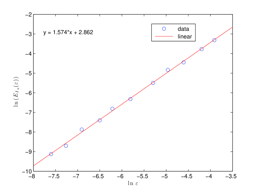
Figure 1: Results of numerical simulation for action variable $I$

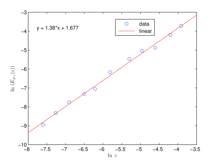
Figure 2: Results of numerical simulation for angle variable $\varphi$

References

- [1] Kevorkian, J. and Cole, J. D.: Multiple Scale and Singular Perturbation Methods. Applied Mathematical Sciences, Vol. 114. Springer-Verlag, 1996.
- [2] Chirikov, B. V.: The passage of a nonlinear oscillatory system through resonance. Sov. Phys., Dokl. 4, 1959, pp. 390-394.
- [3] Bosley, D. L.: An improved matching procedure for transient resonance layers in weakly nonlinear oscillatory systems. Siam J. Appl. Math, Vol. 56, No. 2, 1996, pp. 420-445.
- [4] Alekseev, P. A.: On change of action at passage through a resonance in a quasilinear Hamiltonian system. M.Sc. thesis, Moscow University, 2007.