Extraction of Meson Resonances from Three-pions Photo-production Reactions

Abstract

We have investigated the model dependence of meson resonance properties extracted from the Dalitz-plot analysis of the three-pions photoproduction reactions on the nucleon. Within a unitary model developed in our earlier work, we generate Dalitz-plot distributions as data to perform an isobar model fit that is similar to most of the previous analyses of three-pion production reactions. It is found that the resonance positions from the two models agree well when both fit the data accurately, except for the resonance poles near branch points. The residues of the resonant amplitudes extracted from the two models and by the usual Breit-Wigner procedure agree well only for the isolated resonances with narrow widths. For overlapping resonances, most of the extracted residues could be drastically different. Our results suggest that even with high precision data, the resonance extraction should be based on models within which the amplitude parametrization is constrained by three-particle unitarity condition.

I Introduction

Meson properties are important information for understanding the confinement mechanism of QCD. Thus the investigation of meson spectroscopy has long been an important subject in hadron physics. In recent years, more emphasis has been placed on the study of mesons with quantum numbers beyond the classification of conventional constituent quark model. Such mesons, called exotic mesons, are expected to have explicit gluonic and/or four-quark components in their structure klempt . Therefore the search for exotic mesons has been an important goal in the experiments on $\pi N\to M^{*}N\to\pi\pi\pi N$ at BNL e852 and CERN compass , and $\gamma N\to M^{*}N\to\pi\pi\pi N$ at JLab clas , where the intermediate excited mesons $M^{*}$ could be exotic. However, the existence of exotic mesons, such as $\pi_{1}(1600)$ ($J^{PC}=1^{-+}$) has not been conclusive so far. The forthcoming experiments to be performed at JLab after the 12 GeV upgrade gluex are aimed at providing high precision data for making progress in this direction. In addition to searching for exotic mesons, the new data can also be useful for investigating some mesons that could have exotic structure 3p0 , and can be revealed in their characteristic decay patterns, as discussed in Ref. 3p0 with the ${}^{3}P_{0}$ model.

We are here interested in the excited mesons that decay into three light mesons ($\pi\pi\pi$, $\pi\pi K$, etc.). Since these excited mesons are unstable and couple with multi-mesons continuum to form resonances, the meson spectroscopy can be determined only by analyzing the resonances extracted from the meson production reaction data. Conventionally, these data were analyzed by using the so-called isobar model (IM) in which two of the three mesons form a light flavor excited meson $R$ ($f_{0}$, $\rho$, $K^{*}$, etc.) and the third meson is treated as a spectator of the propagation and the decay of $R$ into two light mesons. This approach obviously violates the three-body unitarity and neglects the coupled-channels effects since the outgoing $R$ can have multiple scattering with the third meson, as illustrated in Fig. 1.

Recently we developed a unitary coupled-channels model 3pi . In this work, we use our model to analyze the $\gamma p\rightarrow M^{*}n\rightarrow\pi^{+}\pi^{+}\pi^{-}n$ reaction, and study the importance of three-body unitarity and coupled-channels effects in extracting the excited meson properties. We consider the reaction where the intermediate $M^{*}$ can be several and can overlap. We will show that while the IM can fit the same Dalitz plot data generated from our unitary model (UM), the extracted resonance parameters are rather different. Our finding indicates the limitation of the IM in establishing the meson spectroscopy.

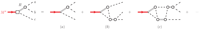
Figure 1: (color online) $M^{*}$-decay amplitude.

This paper is organized as follows. In Sec. II, we present formulae based on our model for identifying the meson resonances in the amplitudes of the $\gamma p\to M^{*}n\to\pi^{+}\pi^{+}\pi^{-}$ reaction, and give the expression for calculating the corresponding Dalitz plots of the cross sections. Our procedure and numerical results are presented in Sec. III, followed by a summary in Sec. IV.

II Formulation

In this paper, we denote pions by $a$, $b$, $c$ and the light excited mesons (such as $f_{0},\rho$ ) by $R$. As illustrated in the left-hand-side of Fig. 2, we assume that the $\gamma N\to abcN^{\prime}$ reaction proceeds via the photo-production of resonant $M^{*}$ states which decay into $cR$ states. Under the three-particle unitarity condition, the propagating $cR$ states experience the multiple-scattering due to the $Z$-diagram mechanism, as illustrated in Fig. 1. The final three pion states are then generated via the $R\rightarrow\pi\pi$ decay mechanism. In the vector meson dominance (VDM) model, one of the production mechanisms can be calculated from a $\pi\rho\rightarrow M^{*}$ and the well known $\pi NN$ vertex, as illustrated in the right-hand-side of Fig. 2. For simplicity, we will calculate the cross section of $\gamma N\to abcN^{\prime}$ reaction using this VDM mechanism, and the $\pi\rho\rightarrow M^{*}$ vertex that reproduce partial width predicted by the ${}^{3}P_{0}$ model of Ref. 3p0 . Accordingly all $M^{*}\rightarrow\pi R$ couplings included in our calculations are also fixed in the same manner. Obviously, this is a simplification, but is sufficient for our present purposes in investigating the importance of three-particle unitarity in extracting $M^{*}$ from the three-pion distribution data. For analyzing the data from CLAS, we need to develop models of other mechanisms. This non-trivial task is beyond the scope of this investigation.

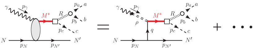
Figure 2: (color online) A graphical representation of the $\gamma N\to abcN^{\prime}$ reaction. The momentum for each particle is shown to explain the notation used in this work. The white square indicates the dressed vertex more explicitly shown in Figs. 3 and 4.

II.1 Cross section

With the momentum variables specified in Fig. 2(b), the cross section of $\gamma N\rightarrow\pi\pi\pi N$ can be written as

$$d\sigma = {1\over v_{\text{rel}}}{1\over 2E_{\gamma}}{1\over 2E_{N}}(2m_{N})^{2}{{\cal B}\over 4}\sum_{s_{N},s_{N^{\prime}},\lambda_{\gamma}}|{\cal M}_{\gamma N\to\pi\pi\pi N^{\prime}}|^{2}$$ (1)

$$\times (2\pi)^{4}\delta^{(4)}(p_{i}-p_{f}){d^{3}p_{N^{\prime}}\over(2\pi)^{3}2E_{N^{\prime}}}{d^{3}p_{a}\over(2\pi)^{3}2E_{a}}{d^{3}p_{b}\over(2\pi)^{3}2E_{b}}{d^{3}p_{c}\over(2\pi)^{3}2E_{c}}\ ,$$

where $v_{\text{rel}}$ is the relative velocity of the initial particles. We used and will use a notation $E_{x}=\sqrt{m_{x}^{2}+\vec{p}^{2}_{x}}$ to denote the free energy for a particle $x$ with the mass $m_{x}$ and the momentum $\vec{p}_{x}$. We denote the Bose factor for the final three pions by ${\cal B}$, and ${\cal B}=1/2$ for $\pi^{+}\pi^{+}\pi^{-}$ final states. We have taken the average of the initial nucleon and photon polarizations (${1\over 4}\sum_{s_{N},\lambda_{\gamma}}$) and the summation over the final nucleon spin ($\sum_{s_{N^{\prime}}}$).

We perform the calculations in the center of mass (CM) frame of the total system. The orientation of the three final pions are specified by the Euler angles $\Omega_{\rm Euler}=(\alpha,\beta,\gamma)$ in the three-meson CM frame (see Eq. (10) and Fig. 1 of Ref. kuhn for the definition of the Euler angles). With some manipulation of the four-body phase-space factor chung ; kuhn , Eq. (1) leads to

$${d\sigma\over dt\ dW\ d\Omega_{\rm Euler}\ dm^{2}_{ab}\ dm^{2}_{bc}} = {{\cal B}m_{N}^{2}\over 4\sqrt{(p_{\gamma}\cdot p_{N})^{2}}}{1\over(4\pi)^{7}}{1\over E_{\text{tot}}\ p^{\text{cm}}_{N}W}\sum_{s_{N},s_{N^{\prime}},\lambda_{\gamma}}|{\cal M}_{\gamma N\to\pi\pi\pi N^{\prime}}|^{2}\ ,$$ (2)

where $d\Omega_{\rm Euler}=d\alpha\ d\cos\beta\ d\gamma$, $E_{\text{tot}}$ is the total energy, $p^{\text{cm}}_{N}$ is the initial nucleon momentum, $t=(p_{N}-p_{N^{\prime}})^{2}$, $W=\sqrt{(p_{a}+p_{b}+p_{c})^{2}}$, and $m^{2}_{ij}=(p_{i}+p_{j})^{2}$. For a given set of $(t,W,\Omega_{\rm Euler})$, we then can calculate the Dalitz-plot distributions of the three out-going pions as functions of two-particle invariant masses $m_{ab}$ and $m_{bc}$ by using Eq. (2).

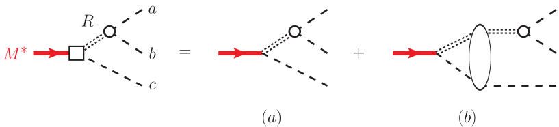
Figure 3: (color online) A graphical representation of the dressed $M^{*}\rightarrow cR$ vertex

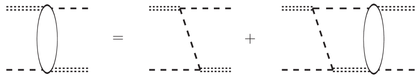
Figure 4: A graphical representation of $cR$ scattering equation.

II.2 Matrix element

With the normalization $\langle{\vec{k}}|{\vec{k}^{\,\,{}^{\prime}}}\rangle=\delta(\vec{k}-\vec{k}^{\,\,{}^{\prime}})$ for the plane-wave state, the invariant amplitude ${\cal M}_{\gamma N\to\pi\pi\pi N^{\prime}}$ in Eq. (2) is related to the scattering amplitude $T_{abcN^{\prime},\gamma N}$ by

$${\cal M}_{\gamma N\to abcN^{\prime}} = -{1\over(2\pi)^{3}}\sqrt{(2\pi)^{3}2E_{\gamma}}\sqrt{(2\pi)^{3}2E_{N}}$$ (3)

$$\times \sqrt{(2\pi)^{3}2E_{a}(p_{a})}\sqrt{(2\pi)^{3}2E_{b}(p_{b})}\sqrt{(2\pi)^{3}2E_{c}(p_{c})}\sqrt{(2\pi)^{3}2E_{N^{\prime}}(p_{N^{\prime}})}\ T_{abcN^{\prime},\gamma N}\ .$$

With the VDM process illustrated in the right-hand-side of Fig. 2, the scattering amplitude in Eq. (3) can be written within our model as

$$T_{abcN^{\prime},\gamma N} = \sum_{\alpha}\sum_{i_{\alpha}j_{\alpha}}\sum_{S^{z}_{M^{*}}}\sum^{\text{cyclic}}_{(a^{\prime}b^{\prime}c^{\prime})}F_{(a^{\prime}b^{\prime})c^{\prime},M^{\ast}_{i_{\alpha}}}(W)\ [G_{M^{*}}(W)]_{i_{\alpha}j_{\alpha}}\ T_{M^{*}_{j_{\alpha}}N^{\prime},\gamma N}(W)\ ,$$ (4)

where $T_{M^{*}N^{\prime},\gamma N}$ is the $M^{*}$ photo-production amplitude, $F_{(ab)c,M^{\ast}}(W)$ is the $M^{*}\rightarrow abc$ decay amplitude, and $G_{M^{*}}(W)$ is the propagator of the $M^{*}$ resonant state. The index $\alpha$ labels a set of quantum numbers (spin, isospin, parity) of $M^{*}$, and $i_{\alpha},j_{\alpha}$ runs over all $M^{*}$s belonging to the set of quantum numbers $\alpha$. The summation over the $M^{*}$ spin orientation is denoted by $\sum_{S^{z}_{M^{*}}}$. The symbol $\sum^{\text{cyclic}}_{(a^{\prime}b^{\prime}c^{\prime})}$ means taking summation over the cyclic permutation, $(a^{\prime}b^{\prime}c^{\prime})=(abc),(cab),(bca)$. As illustrated in Fig. 3, the $M^{*}$ decay amplitude in Eq. (4) consists of two terms

$$F_{(ab)c,M^{*}}(E)=F^{\text{DIR}}_{(ab)c,M^{*}}(E)+F^{\text{FSI}}_{(ab)c,M^{*}}(E)\,.$$ (5)

The direct decay amplitude [Fig. 3(a)] is defined by

$$F^{\text{DIR}}_{(ab)c,M^{*}}(E) = \sum_{R}\sum_{c^{\prime}R^{\prime}}\langle{ab}|f_{ab,R}G_{cR,c^{\prime}R^{\prime}}(E)\Gamma_{c^{\prime}R^{\prime},M^{*}}|{M^{*}}\rangle,$$ (6)

where $f_{ab,R}$ is the $R\rightarrow ab$ vertex interaction, and $\Gamma_{c^{\prime}R^{\prime},M^{*}}|{M^{*}}\rangle$ describes the $M^{*}\rightarrow c^{\prime}R^{\prime}$ decay. The summation in Eq. (6) runs over the particle species and its momentum, spin, and isospin components. The second term of Eq. (5) [Fig. 3(b)] includes the final state interaction (FSI), as required by the three-particle unitarity condition. It has the following expression:

$$F^{\text{FSI}}_{(ab)c,M^{*}}(E) = \sum_{R}\sum_{c^{\prime}R^{\prime}}\sum_{c^{\prime\prime\prime}R^{\prime\prime\prime},c^{\prime\prime}R^{\prime\prime}}\langle{ab}|f_{ab,R}G_{cR,c^{\prime}R^{\prime}}(E)T^{\prime}_{c^{\prime}R^{\prime},c^{\prime\prime\prime}R^{\prime\prime\prime}}(E)G_{c^{\prime\prime\prime}R^{\prime\prime\prime},c^{\prime\prime}R^{\prime\prime}}(E)\Gamma_{c^{\prime\prime}R^{\prime\prime},M^{*}}|{M^{*}}\rangle,$$

where $T^{\prime}_{c^{\prime}R^{\prime},cR}(E)$ is the $cR\rightarrow c^{\prime}R^{\prime}$ scattering amplitudes. As illustrated in Fig. 4, $T^{\prime}_{c^{\prime}R^{\prime},cR}(E)$ is defined by the following coupled-channels scattering equation,

$$T^{\prime}_{c^{\prime}R^{\prime},cR}(E)=Z_{c^{\prime}R^{\prime},cR}(E)+\sum_{c^{\prime\prime\prime}R^{\prime\prime\prime},c^{\prime\prime}R^{\prime\prime}}Z_{c^{\prime}R^{\prime},c^{\prime\prime\prime}R^{\prime\prime\prime}}(E)G_{c^{\prime\prime\prime}R^{\prime\prime\prime},c^{\prime\prime}R^{\prime\prime}}(E)T^{\prime}_{c^{\prime\prime}R^{\prime\prime},cR}(E)\,,$$ (8)

where $Z_{c^{\prime}R^{\prime},cR}$ is the one-particle-exchange $Z$-diagram interaction that is also determined by the $R\to ab$ vertex interaction $f_{ab,R}$

$$Z_{c^{\prime}R^{\prime},cR}(E)=\sum_{c^{\prime\prime}}f_{R^{\prime},cc^{\prime\prime}}\frac{1}{E-E_{c}-E_{c^{\prime}}-E_{c^{\prime\prime}}+i\epsilon}f_{c^{\prime}c^{\prime\prime},R}\ ,$$ (9)

where $c^{\prime\prime}$ is the exchanged meson.

The Green function in Eqs. (6)-(8) is defined by

$$\left[G^{-1}(E)\right]_{c^{\prime}R^{\prime},cR}=\delta_{c^{\prime},c}\left[(E-E_{c}-E_{R})\delta_{R^{\prime},R}-\Sigma_{R^{\prime},R}(E-E_{c})\right]\ ,$$ (10)

where the self-energy of light excited-meson $R$ is determined by the $R\rightarrow ab$ vertex interaction

$$\Sigma_{R^{\prime},R}(w)=\sum_{ab=\pi\pi,K\bar{K}}\langle{R^{\prime}}|f_{R^{\prime},ab}\frac{{\cal B}_{ab}}{w-E_{a}-E_{b}+i\epsilon}f_{ab,R}|{R}\rangle.$$ (11)

Here ${\cal B}_{ab}$ is a factor associated with the Bose symmetry of mesons: ${\cal B}_{ab}=1/2$ if $a$ and $b$ are the identical particles or otherwise ${\cal B}_{ab}=1$.

The $M^{*}$ propagator in Eq. (4) is defined by

$$\left[G^{-1}_{M^{*}}(E)\right]_{ij}=(E-M^{0}_{M^{*}_{i}})\delta_{ij}-\left[\Sigma_{M^{*}}(E)\right]_{ij}\,,$$ (12)

where $M^{0}_{M^{*}_{i}}$ is a bare mass, and the self energy is given by

$$[\Sigma_{M^{*}}(E)]_{ij} = \sum_{cR,c^{\prime}R^{\prime}}\langle{M^{*}_{i}}|\Gamma_{M^{*}_{i},cR}G_{cR,c^{\prime}R^{\prime}}(E)|{\bar{\Gamma}_{c^{\prime}R^{\prime},M^{*}_{j}}}\rangle.$$ (13)

The self energy $[\Sigma_{M^{*}}(E)]_{ij}$ is non-vanishing only when $M^{*}_{i}$ and $M^{*}_{j}$ have the same spin, isospin and parity. In Eq. (13), $|{\bar{\Gamma}_{cR,M^{*}}}\rangle$ is the dressed $M^{*}\to cR$ vertex function defined by

$$|{\bar{\Gamma}_{cR,M^{*}}}\rangle=\sum_{c^{\prime}R^{\prime}}\left[\delta_{cR,c^{\prime}R^{\prime}}+\sum_{c^{\prime\prime}R^{\prime\prime}}T^{\prime}_{cR,c^{\prime\prime}R^{\prime\prime}}G_{c^{\prime\prime}R^{\prime\prime},c^{\prime}R^{\prime}}(E)\right]\Gamma_{c^{\prime}R^{\prime},M^{*}}|{M^{*}}\rangle.$$ (14)

Note that the $M^{*}\rightarrow abc$ amplitude $F_{(ab)c,M^{*}}$ defined by Eqs. (5)-(LABEL:eq:decay-int) is identical to the matrix element $\sum_{Rc^{\prime}R^{\prime}}\langle{ab}|f_{ab,R}G_{cR,c^{\prime}R^{\prime}}|{\bar{\Gamma}_{c^{\prime}R^{\prime},M^{*}}}\rangle$.

To proceed, we need to define $R\leftrightarrow ab$ and $M^{*}\rightarrow cR$ vertex functions. The $R\rightarrow ab$ vertex functions $f_{ab,R}$ have been determined within our model 3pi by fitting the $\pi\pi$ scattering amplitudes up to 2 GeV with $R=f_{0},\rho,f_{2}$. We include $\pi\pi$ and $K\bar{K}$ channels in our model of $\pi\pi$ scattering. While the $\pi\pi\pi$ three-body states appear in $Z$-diagram interactions in Eq. (9), $\pi K\bar{K}$ states appear only in the Green function defined by Eq. (10).

We thus will only consider $cR=\pi f_{0},\pi\rho,\pi f_{2}$ channels. For the bare $M^{*}\leftrightarrow cR$ interaction $\Gamma_{cR,M^{*}}(\vec{p}_{c})$, we use a partial wave expansion,

$$\Gamma_{cR,M^{*}}(\vec{p}_{c})=\sum_{l}\langle{t_{c}t^{z}_{c}t_{R}t^{z}_{R}}|{T_{M^{\ast}}T^{z}_{M^{\ast}}}\rangle\langle{ll^{z},s_{R}s^{z}_{R}}|{S_{M^{\ast}}S^{z}_{M^{\ast}}}\rangle Y^{*}_{l,l^{z}}(-\hat{p}_{c})\Gamma_{(cR)_{l},M^{\ast}}(p_{c})\ ,$$ (15)

where the first (second) parenthesis is isospin (angular momentum) Clebsch-Gordan coefficient; $s_{x}$ ($t_{x}$) is the spin (isospin) of a particle $x$ and $s^{z}_{x}$ ($t^{z}_{x}$) is its $z$-component, and $l$ is the orbital angular momentum of the relative $cR$ motion. The vertex function $\Gamma_{(cR)_{l},M^{\ast}}(p)$ is given with the following parametrization for each partial-wave:

$$\Gamma_{(cR)_{l},M^{*}}(p)=\frac{1}{(2\pi)^{3/2}}C_{(cR)_{l},M^{*}}\sqrt{m_{R}\over 4E_{R}(p)E_{\pi}(p)}\left(\frac{\Lambda^{2}_{(cR)_{l},M^{*}}}{p^{2}+\Lambda^{2}_{(cR)_{l},M^{\ast}}}\right)^{2+(l/2)}\left(\frac{p}{m_{\pi}}\right)^{l}\ .$$ (16)

The parameters $C_{(cR)_{l},M^{*}}$ and $\Lambda_{(cR)_{l},M^{\ast}}$ are chosen to reproduce the partial decay widths of $M^{*}\rightarrow\pi R$ predicted by the ${}^{3}P_{0}$ model of Ref. 3p0 , and will be explained in the next section.

To calculate the $\gamma N\rightarrow\pi\pi\pi N^{\prime}$ amplitude defined by Eq. (4), we also need to calculate the VDM photo-production amplitude $T_{M^{*}N^{\prime},\gamma N}$ illustrated in the right-hand-side of Fig. 2. We use the following interaction Lagrangian to describe the emission of the pion from the nucleon:

$${\cal L}_{\pi NN}=-{f_{\pi NN}\over m_{\pi}}\bar{\psi}_{N}\gamma_{\mu}\gamma_{5}\vec{\tau}\cdot\psi_{N}\partial^{\mu}\vec{\pi}\ ,$$ (17)

where $f^{2}_{\pi NN}(q^{2}=0)/4\pi=0.08$ and $f_{\pi NN}(q^{2})/f_{\pi NN}(0)=1/(1-q^{2}/\Lambda^{2}_{\pi NN})^{2}$. We use $\Lambda_{\pi NN}=700$ MeV which is close to most of the values from the $\pi N$ scattering model sl96 . The photon-$\rho$ contact interaction within the VDM model is defined by the following Lagrangian:

$${\cal L}_{\rho\gamma}={em^{2}_{\rho}\over g_{\rho}}\rho^{3}_{\mu}A^{\mu}\ ,$$ (18)

with $g^{2}_{\rho}/(4\pi)=2.2$.

With the Lagrangians Eqs. (17) and (18), the $\gamma N\rightarrow M^{*}N^{\prime}$ production amplitude in $\gamma N$ CM frame is of the following form

$$T_{M^{*}N^{\prime},\gamma N}(\vec{p}_{M^{*}}\vec{p}_{N^{\prime}};\vec{p}_{\gamma},\vec{p}_{N}) = \sqrt{1\over 2E_{\gamma}E_{N}(\vec{p}_{N})E_{N}(\vec{p}_{N^{\prime}})}\sum_{i}\sqrt{4E_{\rho_{i}}(q)E_{\pi}(q)}\Gamma_{M^{*},\pi\rho_{i}}(\vec{q})\left(e\over g_{\rho}\right)$$ (21)

$$\times{1\over q^{2}-m^{2}_{\pi}}{if_{\pi NN}(q^{2})\over m_{\pi}}\langle\tau_{x}\rangle\ \bar{u}_{\vec{p}_{N^{\prime}}}\ooalign{\hfil/\hfil\crcr$q$}\gamma_{5}u_{\vec{p}_{N}}\ ,$$

where $q=p_{N}-p_{N^{\prime}}$, $u_{\vec{p}}$ is the nucleon spinor. The summation is taken over the first and second bare $\rho$ states. The isospin matrix element between the nucleon states is denoted by $\langle\tau_{x}\rangle=1\ (\sqrt{2})$ for $N=N^{\prime}=p$ ($N=p,N^{\prime}=n$). The $M^{*}\rightarrow\rho_{i}\pi$ vertex function $\Gamma_{M^{*},\pi\rho_{i}}(\vec{q})$ has been defined by Eqs. (15) and (16).

II.3 Isobar-model

We can obtain a model similar to the commonly used IM from the above formula by neglecting the $\pi R$ final state interactions, $F^{\text{FSI}}_{(ab)c,M^{*}}$ in Eq. (5), which are due to the $Z$-diagram mechanism, as illustrated in Fig. 3(b) and Fig. 4. Furthermore, the $M^{*}$ propagator $G_{M^{*}}(W)$ in Eq. (4) are replaced by a Breit-Wigner (BW) form. Explicitly we consider the following expression of the IM,

$$T^{\text{IM}}_{abcN^{\prime},\gamma N} = \sum_{\alpha}\sum_{j_{\alpha}}\sum_{S^{z}_{M^{*}}}\sum^{\text{cyclic}}_{(a^{\prime}b^{\prime}c^{\prime})}F^{\text{DIR}}_{(a^{\prime}b^{\prime})c^{\prime},M^{\ast}_{j_{\alpha}}}(W)\ [G^{\rm BW}_{M^{*}}(W)]_{j_{\alpha}j_{\alpha}}\ T_{M^{*}_{j_{\alpha}}N^{\prime},\gamma N}(W)\ ,$$ (22)

with

$$[G^{\rm BW}_{M^{*}}(W)]_{jj}=-{M^{j}_{\text{BW}}\over(M^{j}_{\text{BW}})^{2}-W^{2}-iM^{j}_{\text{BW}}\Gamma^{j}_{\text{BW}}\left[\left({q\over q^{j}_{\text{BW}}}\right)^{2(L^{j}+1)}\left({(q^{j}_{\text{BW}})^{2}+(\Lambda^{j}_{\text{BW}})^{2}\over q^{2}+(\Lambda^{j}_{\text{BW}})^{2}}\right)^{2}\right]}\ ,$$ (23)

where $q$ is the on-shell momentum satisfying the equation:

$$W=\sqrt{m_{\pi}^{2}+q^{2}}+\sqrt{m_{R_{\text{BW}}}^{2}+q^{2}}\ ,$$ (24)

and $m_{R_{\text{BW}}}=770$ MeV; $q=q^{j}_{\text{BW}}$ when $W=M^{j}_{\text{BW}}$. The integer $L^{j}$ is the lowest allowed orbital angular momentum between the pion and a vector boson for a given $M^{*}_{j}$ at rest. It is noted that the BW $M^{*}$ propagator in Eq. (23) is diagonal with respect to the index $j$, while the $M^{*}$ propagator for the UM given in Eq. (12) can have off-diagonal component, connecting different $M^{*}$s belonging to the same quantum number. Furthermore, whereas the BW $M^{*}$ propagator in Eq. (23) is purely phenomenological, the $M^{*}$ propagator for the UM needs to be given by Eq. (12) as a consequence of three-body unitarity. The IM defined by Eqs. (22) and (23) will be used to extract the resonance parameters from fitting the “data” generated from our UM defined in Sec. II.2.

III Results

Our objective in this paper is to investigate the importance of the three-particle unitarity in determining the excited meson $M^{*}$ properties from fitting the Dalitz-plot distribution data of $3\pi$ states for the $\gamma p\to M^{*}n\to\pi^{+}\pi^{+}\pi^{-}n$ reaction. We do not make an attempt to analyze the CLAS data clas for this reaction here. Thus it is sufficient to consider the VDM production mechanism illustrated in Fig. 2(b). Then we can set up a model by fixing the parameters associated with $M^{*}$ states using partial widths predicted by the ${}^{3}P_{0}$ model of Ref. 3p0 . This will be explained in Sec. III.1.

Once the $M^{*}$ parameters are fixed, we can perform the calculations using the formula presented in previous sections since all parameters needed to calculate the $\pi R\rightarrow\pi R^{\prime}$ amplitudes [Eq. (8)] and $\pi R$ propagator [Eq. (10)] have been determined in our previous work 3pi . The Dalitz plots for the $\pi^{+}\pi^{+}\pi^{-}$ are calculated using Eq. (2), and are presented in Sec. III.2 In Sec. III.3, we describe how the generated Dalitz plots are used as the data to determine the parameters of the IM described in Sec. II.3.

In Sec. III.4, we examine the differences between the resonance parameters extracted with our UM and those from the fitted IM. Their differences will indicate the importance of the three-particle unitarity in determining the excited meson $M^{*}$ properties from fitting the Dalitz-plot distribution data of the $3\pi$ states for the $\gamma p\to\pi^{+}\pi^{+}\pi^{-}n$ reaction.

III.1 Determination of the $M^{*}$ parameters

In our UM, we consider the $\pi R$ partial waves that are found to be necessary to fit the CLAS data for $1.0<W<1.36$ GeV clas . We thus have one or two bare $M^{*}$ states for four partial waves: $J^{PC}=1^{++}$ [$a_{1}(1230)$, $a_{1}(1700)$], $2^{++}$ [$a_{2}(1320)$, $a_{2}(1700)$], $2^{-+}$ [$\pi_{2}(1670)$, $\pi_{2}(1800)$], $1^{-+}$ [$\pi_{1}(1600)$]. We assume that our bare $M^{*}$ states can be identified with excited meson states of the $q\bar{q}$ excitation type listed in Ref. 3p0 , and that their bare $M^{*}\to\pi R$ couplings are fixed so that the partial decay widths predicted by the ${}^{3}P_{0}$ model 3p0 are reproduced; we use the formula given in Appendix I of Ref. msl to calculate the partial widths. We also assume that the daughter $\pi R$ states have the lowest allowed orbital angular momenta. The bare masses $M^{0}_{M^{*}}$ are also identified with the excited meson masses listed in Ref. 3p0 . The only exception is the $\pi_{1}(1600)$ that is speculated to be a hybrid state. In this investigation we use the mass and partial widths for $\pi_{1}(1600)$ given in Ref. IKP . For simplicity, we set all $M^{*}\to\pi R$ cutoffs to $\Lambda_{(\pi R)_{l},M^{*}}=1$ GeV. With the above specifications, the parameters for our UM are fixed.

III.2 Calculations of Dalitz plots

We use Eq. (2) to generate the Dalitz-plot distributions of $\pi^{+}\pi^{+}\pi^{-}$ for the $\gamma p\rightarrow\pi^{+}\pi^{+}\pi^{-}n$ reaction at the photon energy $E_{\gamma}=5$ GeV and the momentum-transfer $t=-0.4$ GeV². This is the kinematics considered in the CLAS analysis clas .

We next need to specify the Euler angles [$\Omega_{\rm Euler}$ in Eq. (2)] that define the orientation of the three-pion plane in their center of mass system. Experimentally, it would be preferred to choose an orientation where the three pions have less chance to interact with the final nucleon. Thus we choose the Euler angle $\beta$ such that the three-pion plane is perpendicular to the direction of the final nucleon. Because the cross section does not depend on $\alpha$, we set $\alpha=0$. The remaining Euler angle $\gamma$ gives the rotation of the three pions around their CM on the plane specified by $\alpha$ and $\beta$. We calculate Dalitz plots by varying $\gamma$ in the range $0\leq\gamma\leq 2\pi$.

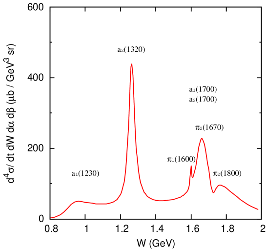
Figure 5: (color online) $W$-dependence of integrated Dalitz-plot distribution of the three pions for the $\gamma p\to M^{*}n\to\pi^{+}\pi^{+}\pi^{-}n$ reaction, obtained from Eq. (2) by integrating over the kinematical variables $m^{2}_{ab},m^{2}_{bc}$ and $\gamma$. The other variables are $t=-0.4$ GeV², $\alpha=0$, and $\beta$ is fixed as explained in the text.

To see the contributions of the considered resonances to the generated data, we show in Fig. 5 the cross sections calculated from Eq. (2) by integrating over $m^{2}_{ab},m^{2}_{bc}$ and $\gamma$. We see a broad bump at $W\sim 0.95$ GeV due to $a_{1}(1230)$, a highest peak at $W\sim 1.25$ GeV due to $a_{2}(1320)$. The second highest peak at $W\sim 1.65$ GeV is due to $a_{1}(1700)$ and $a_{2}(1700)$. The gap at $W\sim 1.7$ GeV is due to an interference between $\pi_{2}(1670)$ and $\pi_{2}(1800)$. The exotic $\pi_{1}(1600)$ is clearly visible as a small spike at $W\sim 1.6$ GeV. Clearly it is a highly non-trivial task to fit the generated Dalitz-plot distribution data, in particular, in the region 1.6 GeV $\leq W\leq$ 1.8 GeV where the contributions from several resonances overlap strongly.

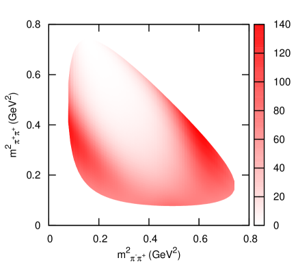
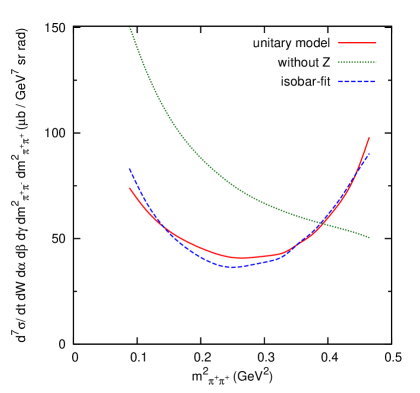
Figure 6: (color online) (left) Dalitz-plot distribution of $3\pi$ [Eq. (2); unit: $\mu{\rm b}/{\rm GeV}^{7}{\rm sr\>rad}$] from our UM for the $\gamma p\to\pi^{+}\pi^{+}\pi^{-}n$ reaction at $W$ = 1 GeV near $a_{1}(1230)$ peak, $\cos\beta=-0.37$, and $\gamma=90^{\circ}$. (right) One slice cut of the Dalitz plot on the left at $m^{2}_{\pi^{-}\pi^{+}}=0.51$ GeV².

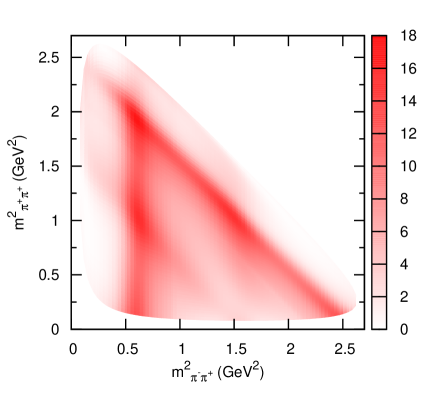
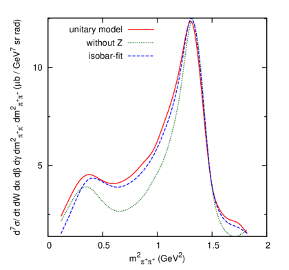
Figure 7: (color online) Dalitz-plot distribution of $3\pi$ at $W$ = 1.76 GeV near $\pi_{2}(1800)$ peaks, $\cos\beta=-0.77$, and $\gamma=173^{\circ}$. On the right, one slice cut of the Dalitz plot on the left is at $m^{2}_{\pi^{-}\pi^{+}}=1.23$ GeV². The other features are the same as those in Fig. 6.

Table 1: Bare masses $M^{0}_{M^{\ast}}$ (MeV) as well as couplings $C_{(\pi R^{LI}_{i})_{l},M^{*}}$ (dimensionless) and cutoffs $\Lambda_{\pi R,M^{\ast}}$ (MeV) of Eq. (16), for the $M^{\ast}=\pi_{2}(1670)$, $\pi_{2}(1800)$, and $\pi_{1}(1600)$ from the UM and those from the IM are compared. $R^{LI}_{i}$ denotes the $i$-th bare $R$ state with the spin $L$ and the isospin $I$. $l$ denotes the orbital angular momentum between $R^{LI}_{i}$ and $\pi$. See Table I of Ref. 3pi for the properties of $R^{LI}_{i}$. For the IM, the BW mass ($M_{\text{BW}}$), width ($\Gamma_{\text{BW}}$) and the cutoff ($\Lambda_{\text{BW}}$) are also listed.

	$\pi_{2}(1670)$		$\pi_{2}(1800)$		$\pi_{1}(1600)$
	UM	IM	UM	IM	UM	IM
$M^{0}_{M^{*}}$ ($M_{\text{BW}}$)	1670.	1815.	1800.	1727.	1600.	1599.
($\Gamma_{\text{BW}}$)	-	565.	-	69.	-	8.
($\Lambda_{\text{BW}}$)	-	1005.	-	1144.	-	651.
$C_{(\pi R^{00}_{1})_{2},M^{*}}$	-	0.18 + 0.05$i$	0.13	$-$ 0.08 + 0.02$i$	-	-
$\Lambda_{(\pi R^{00}_{1})_{2},M^{*}}$	-	1999.	1000.	1039.	-	-
$C_{(\pi R^{00}_{2})_{2},M^{*}}$	-	0.02 + 0.04$i$	-	$-$ 0.07 + 0.15$i$	-	-
$\Lambda_{(\pi R^{00}_{2})_{2},M^{*}}$	-	1991.	-	649.	-	-
$C_{(\pi R^{11}_{1})_{1},M^{*}}$	3.94	4.98 + 0.60$i$	4.84	$-$ 1.08 + 0.04$i$	1.01	1.17 $-$ 0.60$i$
$\Lambda_{(\pi R^{11}_{1}),M^{*}}$	1000.	1289.	1000.	1719.	1000	1116.
$C_{(\pi R^{11}_{2})_{1},M^{*}}$	-	$-$ 2.29 $-$ 6.66$i$	-	2.64 + 0.30$i$	-	0.07 + 0.16$i$
$C_{(\pi R^{11}_{2})_{3},M^{*}}$	-	$-$ 0.02 $-$ 0.02$i$	-	$-$ 0.01 + 0.00$i$	-	-
$\Lambda_{(\pi R^{11}_{2}),M^{*}}$	-	884.	-	1007.	-	525.
$C_{(\pi R^{20}_{1})_{0},M^{*}}$	8.39	15.09 + 1.29$i$	9.29	$-$ 3.66 $-$ 0.55$i$	-	-
$C_{(\pi R^{20}_{1})_{2},M^{*}}$	-	0.11 + 0.02$i$	-	0.00 + 0.00$i$	-	-
$\Lambda_{(\pi R^{20}_{1}),M^{*}}$	1000.	817.	1000.	1077.	-	-

III.3 Fit

With the kinematics described above, the Dalitz-plot distribution of the three pions are generated with Eq. (2) by varying the variables $W$, $\gamma$ (one of the Euler angles), $m^{2}_{ab}$ and $m^{2}_{bc}$. We calculate the cross sections at kinematical points that are uniformly distributed in the space spanned by these kinematical variables. The calculated cross sections at these points are regarded as the ‘data’ in determining the parameters of the IM defined in Sec. II.3.

As examples, we show in the left sides of Figs. 6 and 7 the generated Dalitz-plot distributions in the $m^{2}_{\pi^{-}\pi^{+}}$-$m^{2}_{\pi^{+}\pi^{+}}$ plane at $W=1$ GeV and $W=1.76$ GeV, respectively. The Dalitz-plot distributions largely depend on $\gamma$ both in shape and magnitude. Thus in these figures, we choose $\gamma$ where the Dalitz plot has the highest peak at the value of $W$.

In the right-hand sides of Figs. 6 and 7, the solid curves (unitary model) are the distribution at a fixed $m^{2}_{\pi^{+}\pi^{-}}$ of the $x$-axis of the Dalitz plot on the left. The dotted curves (without $Z$) are obtained by turning off the $Z$-diagram mechanism in our unitary calculations. Clearly, the effect of the $Z$-diagram mechanism, which is the necessary consequence of three-particle unitarity condition, is important, especially in Fig. 6 where $a_{1}(1230)$ dominates.

For fitting the data with $\chi^{2}$-minimization, we need to assign an error to each data point. We use the same error for all data points belonging to the same $W$. For a given $W$, we use 5% of the highest value in the Dalitz plot distributions as the error.

We adjust the BW parameters $M_{\text{BW}}$, $\Gamma_{\text{BW}}$ and $\Lambda_{\text{BW}}$ in Eq. (23), and all $M^{*}\to\pi R$ couplings constants $C_{(\pi R)_{L},M^{*}}$ and cutoffs $\Lambda_{(\pi R)_{L},M^{*}}$ to fit the Dalitz plots generated with our UM. First we tried fitting with real $M^{*}\to\pi R$ couplings, but no satisfactory fit is obtained. Thus we allow $M^{*}\to\pi R$ couplings to be complex, as usually done in the IM analysis. To get high precision fits, we find that the IM needs to include more partial waves in the $M^{*}\rightarrow\pi R$ transition. This can be seen in Table 1 in comparing the parameters of the starting UM and IM. The comparisons of the parameters for the other $M^{*}$ states are similar and therefore need not to be given here. (Note that the parameters of the UM are from selecting only few partial waves which have information from the ${}^{3}P_{0}$ model. So the Table 1 should not be used in comparing the merits of each model. Namely, if we start from the data generated from the IM with few partial waves, then the UM fits will also need more partial waves. )

We find that even with much more partial waves in the fit, as seen in Table 1, the IM still cannot fit data well. The high precision fits are obtained only when we add at each $W$ a flat and non-interfering background to the Dalitz-plot distributions calculated from the IM. The background contribution could in principle depend on kinematics and interfere with the resonance contributions. However, we follow the common practice of previous IM analyses, e.g., Refs. e852 ; compass ; clas , to introduce the background contribution. In Fig. 8, we show the background contribution to the integrated Dalitz-plot distribution [$m^{2}_{\pi^{+}\pi^{-}}$, $m^{2}_{\pi^{+}\pi^{+}}$ and $\gamma$ are integrated over from Eq. (2)] which can be compared to Fig. 5. The background contribution is highly $W$-dependent. The largest contribution relative to the full Dalitz-plot distribution (the background plus the IM) is at $W=1140$ MeV by 37%. Below the $a_{2}(1320)$ [$a_{2}(1700)$] peak, the contribution is 22% [29%]. In some regions, on the other hand, the background contribution is almost zero as can be seen in the figure.

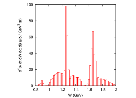
Figure 8: (color online) The contribution from the constant background cross sections to the integrated Dalitz plot obtained from Eq. (2) by integrating over $m^{2}_{\pi^{+}\pi^{-}}$, $m^{2}_{\pi^{+}\pi^{+}}$ and $\gamma$.

A good quality of fit has been obtained with the IM. The IM gives Dalitz-plot distributions that are not distinguishable from the left-hand-side of Figs. 6 and 7 of the UM. The good fits can be seen from comparing the solid (unitary model) and dashed (isobar fit) curves in the right-hand-side of the same figures.

III.4 $M^{*}$ Parameters

Table 2: Pole positions $M^{\text{UM}}_{R}$ from the UM and $M^{\text{IM}}_{R}$ from the IM are compared. ${M^{\text{IM(BW)}}_{R}}$ are the BW masses and widths $(M_{\text{BW}},-\Gamma_{\text{BW}}/2)$ from the IM. All are in unit of MeV.

$M^{*}$	$M^{0}_{M^{*}}$	$M_{R}^{\text{UM}}$	$M^{\text{IM}}_{R}$	$M^{\text{IM(BW)}}_{R}$
$a_{1}$	1230	(913, $-$69)	(940,$-$64)	(1111,$-$600)
	–	(1443, $-$342)	(1201,$-$212)	(1391,$-$389)
	1700	(1658,$-$53)	(1672,$-$59)	(1676,$-$59)
$a_{2}$	1320	(1263, $-$21)	(1262,$-$22)	(1267,$-$24)
	1700	(1652,$-$38)	(1657,$-$48)	(1668,$-$52)
$\pi_{2}$	1670	(1786,$-$228)	(1701,$-$220)	(1815,$-$283)
	1800	(1722,$-$26)	(1724,$-$34)	(1726,$-$34)
$\pi_{1}$	1600	(1599, $-$4)	(1599,$-$4)	(1599,$-$4)

We apply the analytic continuation method developed in Ref. ssl-I to extract the resonance pole positions from searching for the solutions of ${\rm det}[G^{-1}_{M^{*}}(E)]=0$ of Eq. (12) for our UM and $[G^{BW}_{M^{*}}(E)]^{-1}=0$ of Eq. (23) for the IM. The extracted poles $M_{R}$ for the UM and $M^{IM}_{R}$ for IM are compared in Table 2. For the UM, we also list their bare masses $M^{0}_{M^{*}}$. For $a_{1}$, we see that two bare states evolve into three resonance poles. The situation is similar to $P_{11}$ nucleon resonances reported in Ref. sjklms10 . In the last column, we also list the BW positions $(M_{BW},-\Gamma_{BW}/2)$.

The results shown in Table 2 are similar to what we have observed in other analyses: if the data are fitted equally well, the extracted resonance positions are rather insensitive to the parametrization of the amplitudes as far as the singularities of the scattering amplitudes like branch points are far from the resonance pole. Here we find a significant difference between UM and IM in two poles associated with second $a_{1}$ (second row in Table 2). The pole position of $a_{1}$ at $1443-i342$ MeV of the UM is close to the branch points at $1387-101i$ MeV for the $\pi$-$f_{2}(1270)$ channel and $1487-167i$ MeV for the $\pi$-$f_{0}(1370)$ channel. Thus the resonance shape of the amplitude at real $W$ are distorted by those singularity at the complex energies. On the other hand, BW model has only a single complex energy surface, and has no branch cut. We have observed sjklms10 the similar situation in the study of Roper nucleon resonance $N^{*}(1440)$.

For $a_{2}$, we see from Fig. 5 that two resonances for this partial waves are well separated. Furthermore, $a_{2}(1320)$ is a very pronounced and isolated resonance, like the $\Delta(1232)$ resonance. Thus it is not surprising to see that the resonance positions for $a_{2}(1320)$ from two models are almost identical and the BW value is also very close to the pole position.

For $\pi_{2}$, we assign the wide resonance as $\pi_{2}(1670)$ and the narrow one as $\pi_{2}(1800)$ in Table 2. In UM, the mass of the wide resonance ($1786-228i$ MeV) is higher than that of the narrow one ($1722-26i$ MeV), while the order of two resonances is reversed in IM. Though IM reproduces well the data of Dalitz plot, the resonance positions for overlapping resonances are sensitive to the reaction dynamics.

We next compare the residues of the partial-wave amplitudes of $\gamma\pi\rightarrow R\pi$ transition evaluated at the resonance positions. To proceed, we first note that the total amplitude of ${\gamma N\to\pi\pi\pi N^{\prime}}$ defined by Eqs. (4)-(LABEL:eq:decay-int) can be cast into the following form:

$$T_{abcN^{\prime},\gamma N} = \sum^{\text{cyclic}}_{(a^{\prime}b^{\prime}c^{\prime})}\sum_{R^{\prime}}<a^{\prime}b^{\prime}c^{\prime}N^{\prime}|f_{a^{\prime}b^{\prime},R^{\prime}}\sum_{c^{\prime\prime}R^{\prime\prime}}G_{c^{\prime}R^{\prime},c^{\prime\prime}R^{\prime\prime}}T^{0}_{c^{\prime\prime}R^{\prime\prime}N^{\prime},\gamma N}(W)\ ,|\gamma N>$$ (25)

with

$$T^{0}_{c^{\prime}R^{\prime}N^{\prime},\gamma N}(W)=\sum_{\alpha}\sum_{j_{\alpha}k_{\alpha}}\sum_{S^{z}_{M^{*}}}\bar{\Gamma}_{c^{\prime}R^{\prime},M^{*}_{j_{\alpha}}}[G_{M^{*}}(W)]_{j_{\alpha}k_{\alpha}}T_{M^{*}_{k_{\alpha}}N^{\prime},\gamma N}(W)\ .$$ (26)

By using Eq. (21) for $T_{M^{*}N^{\prime},\gamma N}(W)$ and performing the partial-wave expansion, the following partial wave amplitude $T^{\alpha}_{(\gamma\pi)_{L_{i}}\to(R^{LI}_{i}\pi)_{L_{f}}}(W)$ can be separated from $T^{0}_{c^{\prime}R^{\prime}N^{\prime},\gamma N}(W)$:

$$T^{\alpha}_{(\gamma\pi)_{L_{i}}\to(R^{LI}_{i}\pi)_{L_{f}}}(W) = \sum_{j_{\alpha}k_{\alpha}}\bar{\Gamma}_{(R^{LI}_{i}\pi)_{L_{f}},M_{j_{\alpha}}^{*}}(W,p_{R^{LI}_{i}})$$ (27)

$$\times \left[G_{M^{*}}(W)\right]_{j_{\alpha}k_{\alpha}}\left({e\over g_{\rho}}\sum_{\rho^{\prime}}\sqrt{E_{\rho^{\prime}}(p_{\rho^{\prime}})\over E_{\gamma}(p_{\rho^{\prime}})}{\Gamma}_{M_{k_{\alpha}}^{*},(\rho^{\prime}\pi)_{L_{i}}}(p_{\rho^{\prime}})\right)\ ,$$

where $L_{i}$ ($L_{f}$) is the orbital angular momentum of $\gamma\pi$ ($R^{LI}_{i}\pi$). The symbol $p_{R^{LI}_{i}}$ ($p_{\rho^{\prime}}$) denotes the on-shell momentum of ${R^{LI}_{i}}$ ($\rho^{\prime}$) that satisfies $W=M_{R}=E_{R^{LI}_{i}}(p_{R^{LI}_{i}})+E_{\pi}(p_{R^{LI}_{i}})$ where the bare mass of ${R^{LI}_{i}}$ in our model is used to calculate the energy $E_{R^{LI}_{i}}(p_{R^{LI}_{i}})$.

The residue at each pole position $M_{R}$ is then defined by a contour integration along a closed path ($C_{M_{R}}$) around the pole position $M_{R}$. We further multiply it by phase-space factors to define

$$B^{\alpha,M_{R}}\left((\gamma\pi)_{L_{i}}\to(R^{LI}_{i}\pi)_{L_{f}}\right) = -\sqrt{\rho_{\gamma\pi}(M_{R})\ \rho_{R^{LI}_{i}\pi}(M_{R})}\oint_{C_{M_{R}}}\!\!\!d\bar{W}\ T^{\alpha}_{(\gamma\pi)_{L_{i}}\to(R^{LI}_{i}\pi)_{L_{f}}}(\bar{W})\ ,$$ (28)

where the phase space factors are

$$\rho_{R\pi}(W) = \pi{p_{R}E_{R}(p_{R})E_{\pi}(p_{R})\over W}\ ,$$

$$\rho_{\gamma\pi}(W) = \pi\frac{p^{2}_{\gamma}E_{\pi}(p_{\gamma})}{W}.$$ (29)

For the IM, we can cast Eq. (22) into the same form of Eqs. (25)-(27). It is straightforward to see that the resulting $\gamma\pi\rightarrow\pi R$ amplitude is

$$T^{\alpha(\text{IM})}_{(\gamma\pi)_{L_{i}}\to(R^{LI}_{i}\pi)_{L_{f}}}(W) = \sum_{j_{\alpha}}\Gamma_{(R^{LI}_{i}\pi)_{L_{f}},M^{*}_{j_{\alpha}}}(p_{R^{LI}_{i}})$$ (30)

$$\times [G^{BW}_{M^{*}}(W)]_{j_{\alpha}j_{\alpha}}\left({e\over g_{\rho}}\sum_{\rho^{\prime}}\sqrt{E_{\rho^{\prime}}(p_{\rho^{\prime}})\over E_{\gamma}(p_{\rho^{\prime}})}\Gamma_{M^{*}_{j_{\alpha}},(\rho^{\prime}\pi)_{L_{i}}}(p_{\rho^{\prime}})\right)\ ,$$

where $G^{BW}_{M^{*}}(W)$ is given in Eq. (23). Its residue can be measured by using Eq. (28) with the replacement $T^{\alpha}_{(\gamma\pi)_{L_{i}}\to(R^{LI}_{i}\pi)_{L_{f}}}(W)\rightarrow T^{\alpha(\text{IM})}_{(\gamma\pi)_{L_{i}}\to(R^{LI}_{i}\pi)_{L_{f}}}(W)$.

Following the usual procedure, the residue of the BW parametrization at $W=M_{\text{BW}}$ is then obtained from Eq. (30) by replacing $G^{\text{BW}}_{M^{*}}(W)$ with $1/2$. Multiplying the same phase factors, we then define for the BW:

$$B^{\alpha,M^{j_{\alpha}}_{\text{BW}}}_{\rm IM(BW)}\left((\gamma\pi)_{L_{i}}\to(R^{LI}_{i}\pi)_{L_{f}}\right) = -{1\over 2}\sqrt{\rho_{\gamma\pi}(M^{j_{\alpha}}_{\text{BW}})\ \rho_{R^{LI}_{i}\pi}(M^{j_{\alpha}}_{\text{BW}})}\ \Gamma_{(R^{LI}_{i}\pi)_{L_{f}},M^{*}_{j_{\alpha}}}(p_{R^{LI}_{i}})$$ (31)

$$\times \left({e\over g_{\rho}}\sum_{\rho^{\prime}}\sqrt{E_{\rho^{\prime}}(p_{\rho^{\prime}})\over E_{\gamma}(p_{\rho^{\prime}})}\Gamma_{M^{*}_{j_{\alpha}},(\rho^{\prime}\pi)_{L_{i}}}(p_{\rho^{\prime}})\right)\ ,$$

where the on-shell momenta are for the BW mass ($M_{\text{BW}}$) taken as the total energy.

We have determined the residues for $M^{*}$s of UM and IM using Eq. (28), and also the conventional BW residues for IM using Eq. (31). In Table 3 we present only results which are useful in revealing the essential differences between these three residues. Because the overall phase is arbitrary, we choose the overall phase for IM such that the phases of $B(\gamma\pi\to R^{11}_{1}\pi)$ for the most prominent $a_{2}(1320)$ are the same for all three cases in this table. Guided by the results of the $W$-dependence of cross sections shown in Fig. 5 and the pole positions shown in Table 2, we focus on three different situations: (a) the resonances are broad such as the second $a_{1}(1230)$; (b) resonances in the same partial wave are narrow and isolated such as $a_{2}(1320)$ and $a_{2}(1700)$; (c) resonances in the same partial wave overlap such as $\pi_{2}(1670)$ and $\pi_{2}(1800)$.

We see that for the broad resonance 2nd-$a_{1}(1230)$, the extracted residues are drastically different between UM and IM. This is of course partly due to the difficulties in getting the same pole position for the reason discussed in this subsection. For the $a_{2}(1320)$ that gives the very pronounced peak in Fig. 5, both the resonance positions and residues agree almost perfectly between UM and IM. This is not surprising since it is similar to the situation of the well known $\Delta(1232)$ resonance in the $\pi N$ scattering. For the $a_{2}(1700)$, there is some difference in resonance positions and residues. Since the residues from UM and IM are from loop integration around the pole position as given in Eq. (28), their differences originate from the differences in their amplitudes near the pole position. This is illustrated in Fig. 9 for this resonance. We see that the amplitudes from UM and IM are rather different near their pole positions and hence lead to the differences in residues which are calculated from loop integration of the amplitude around the pole position. This indicates that the resonance properties extracted from data are not independent of analysis method, and thus it is essential to have a parametrization of the amplitude with theoretical constraint. Finally, for $\pi_{2}(1670)$ and $\pi_{2}(1800)$, it is not surprising to see that the phases of their residues from UM and IM are very different since two resonances are overlapping.

Table 3: The pole positions $M_{R}$ and the weighted-residues $B(\gamma\pi\rightarrow\pi R^{LI}_{i})$ defined in Eq. (28) from UM and IM fit are compared. $R^{LI}_{i}$ denotes the $i$-th bare $R$ state with the spin $L$ and the isospin $I$. For $M_{R}$, they are listed as $({\rm Re}(M_{R}),{\rm Im}(M_{R}))$ [MeV]. The column under IM(BW) are from IM but using the usual BW procedure with their masses listed as $M_{R}=(M_{BW},-\Gamma_{BW}/2$). For the weighted-residues, we list as ($|B|$ [MeV], $\phi$ [deg]) of the expression $B(\gamma\pi\rightarrow\pi R)=|B|e^{i\phi}$. The overall phase for IM is chosen such that the phases of $B(\gamma\pi\to R^{11}_{1}\pi)$ for the most prominent $a_{2}(1320)$ are the same as UM.

$M^{*}$			$(L_{i},L_{f})$	UM	IM (pole)	IM (BW)
2nd-$a_{1}$(1230)	$M_{R}$			$(1443,-342)$	$(1201,-212)$	$(1391,-389)$
		$B(\gamma\pi\to\pi R^{11}_{1})$	(0,0)	$64.1,\ -67.$	$28.4,\ -171.$	$33.6,\ -150.$
		$B(\gamma\pi\to\pi R^{11}_{1})$	(0,2)	$8.1,\ 34.$	$0.0,\ 180.$	$0.0,\ 180.$
$a_{2}(1320)$	$M_{R}$			$(1263,-21)$	$(1262,-22)$	$(1267,-24)$
		$B(\gamma\pi\to\pi R^{11}_{1})$	(2,2)	$6.2,\ 171.$	$6.2,\ 171.$	$6.7,\ 171.$
$a_{2}(1700)$	$M_{R}$			$(1652,-38)$	$(1657,-48)$	$(1668,-52)$
		$B(\gamma\pi\to\pi R^{11}_{1})$	(2,2)	$9.4,\ 147.$	$6.5,\ 139.$	$7.1,\ 140.$
$\pi_{2}$(1670)	$M_{R}$			$(1785,-229)$	$(1701,-220)$	$(1815,-283)$
		$B(\gamma\pi\to\pi R^{00}_{1})$	(1,2)	$2.0,\ -123.$	$4.5,\ 129.$	$5.4,\ 176.$
		$B(\gamma\pi\to\pi R^{11}_{1})$	(1,1)	$31.8,\ -134.$	$37.6,\ 167.$	$38.6,\ 168.$
		$B(\gamma\pi\to\pi R^{11}_{1})$	(1,3)	$1.9,\ -101.$	$0.6,\ 153.$	$0.7,\ 176.$
$\pi_{2}$(1800)	$M_{R}$			$(1722,-26)$	$(1724,-34)$	$(1726,-34)$
		$B(\gamma\pi\to\pi R^{00}_{1})$	(1,2)	$0.6,\ 73.$	$0.6,\ -26.$	$0.6,\ -35.$
		$B(\gamma\pi\to\pi R^{11}_{1})$	(1,1)	$4.5,\ 4.$	$4.3,\ -7.$	$4.3,\ -21.$
		$B(\gamma\pi\to\pi R^{11}_{1})$	(1,3)	$0.2,\ 14.$	$0.0,\ 180.$	$0.0,\ 180.$

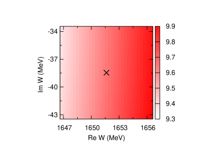
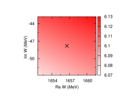
Figure 9: (color online) The real part of $(W-M_{R})T^{\alpha}_{(\gamma\pi)_{2}\to(R^{11}_{1}\pi)_{2}}(W)$ [10^-6 MeV^-1/2] for $a_{2}(1700)$ from the UM (left), and from the isobar plus BW model (right). The pole position for $a_{2}(1700)$ is indicated by the cross. The resonant amplitude, $T^{\alpha}_{(\gamma\pi)_{2}\to(R^{11}_{1}\pi)_{2}}(W)$, is defined in Eq. (27).

IV Summary

We applied the unitary coupled-channels model developed in Ref. 3pi to investigate the issues concerning the extraction of meson resonances from the three-pions photoproduction reaction on the nucleon. Our aim here is to examine the importance of the three-body unitarity, which is not accounted for rigorously in the commonly used IM analyses for the resonance extraction. This has been done by comparing the resonance parameters extracted with our UM and an IM both of which reproduce the same Dalitz plots over relevant kinematical region. We also compare the resonance parameters with the usual BW parameters of the same IM.

We found that the good IM fits to the Dalitz plots generated from the UM can be achieved only when the $M^{*}\to\pi R$ coupling are allowed to become complex and a flat background is added at each $W$. The resonance positions from the two models agree well, except for the resonance poles whose tails are partly blocked by branch cuts on the Riemann surface from reaching at the physical real $W$ axis and for the overlapping resonances. The residues of the resonant amplitudes extracted from the two models and those from the usual BW procedure agree well only for the isolated resonances with narrow widths. Most of the extracted residues for overlapping resonances could be drastically different. Our results suggest that even with high precision data, the resonance extraction should be based on models within which the amplitude parametrization is constrained by three-particle unitarity condition.