Quantum computation with surface-state electrons by rapid population passages

Abstract

Quantum computation requires coherently controlling the evolutions of qubits. Usually, these manipulations are implemented by precisely designing the durations (such as the $\pi$-pulses) of the Rabi oscillations and tunable interbit coupling. Relaxing this requirement, here we show that the desired population transfers between the logic states can be deterministically realized (and thus quantum computation could be implemented) both adiabatically and non-adiabatically, by performing the duration-insensitive quantum manipulations. Our proposal is specifically demonstrated with the surface-state of electrons floating on the liquid helium, but could also be applied to the other artificially controllable systems for quantum computing.

PACS numbers: 33.80.Be, 03.67.Lx, 32.80.Qk,

I Introduction

With the advent of the integrated circuits technology, the components of the classical computer become smaller and smaller and inevitably quantum effects such as quantum interference have to be met. Due to these quantum effects, the usual (classical) computing technology might be invalid and computation based on the quantum laws opens a new chapter to overcome the limits of classical computing Lloyds . Indeed, it has been shown that quantum computation could solve effectively certain problems (e.g., factoring large numbers Shor and searching databases Grover ), which could not be solved by classical algorithms. Different from the bits in classical computer, the qubits in a quantum computer are made by the controlled two-level quantum systems and could be prepared at the superpositions of their basis states Peter . Therefore, quantum computer provides an automatically-parallel computing and thus is much more powerful than the classical computer.

Basically, the central task for quantum computing is to coherently control the transitions between the quantum logic states for implementing various gate operations. Generally, there are two well-known approaches to realize the population transfers between two quantum states; one makes use of the Rabi oscillations and the other is based on population passages Fleischhauer ; Shore . In the first way a constant-intensity resonant driving is applied to the two-state system, and the population of the target state can undergo a periodic variation with the Rabi frequency. This implies that, by properly choosing the pulse duration $T$ (such that the pulse area $\Omega T$ is an odd multiple of $\pi$), the population of the initial state can be completely transferred into the target state. Obviously, the main disadvantage of this method is that the pulse area should be precisely designed. Alternatively, in the second approach the population of the initial state is transferred into the target state by utilizing various population passage techniques Bergmann . Importantly, both the adiabatical and non-adiabatical passages are insensitive to the areas of the applied pulses, and thus there is no need to design the exact durations of the applied pulses. By this way, the desired quantum manipulations for quantum computing could be realized more easily, at least in principle.

Usually, the population passages are demonstrated by various adiabatic manipulations, owing to its relative simplicity. For example, one of the adiabatic passage technique called Stark-chirped rapid adiabatic passage (SCRAP) has been attracting a lot of attention in modern atomic, molecular and optical physics Rickes ; Rangelov ; Yatsenko . Different from the other adiabatical passages such as the stimulated Raman adiabatical passage (STIRAP), the Stark shifts in the SCRAP caused by the external pulses are beneficial to create the desired level-crossings needed for population passages Yatsenko . Also, unlike the technique in STIRAP with the assistants of various intermediate states, the population transfers between the two selected quantum states can be directly realized by just controlling the relative intensity and delay time between the two applied pulses. Therefore, the operations of SCRAPs are relatively simple and have been utilizing in various quantum state engineerings based on population passages. Certainly, the adiabatic requirement in the SCRAP is a fundamental hurdle for its various potential applications. Under such a limit, the applied pulse operations should be sufficiently slow such that the evolution of the manipulated quantum state is adiabatic. However, the practically-existing finite decoherence time of the manipulated quantum system requires that the applied operations should be sufficiently fast such that the operations could be completed before the manipulated quantum superposed state decoheres. Therefore, relaxing the adiabatic condition is useful to experimentally implement the fast population transfers for desired quantum computing.

In this paper, by making use of the evolution-time insensitivity, we propose the adiabatic and non-adiabatic population passages to implement the quantum computation with electrons floating on the liquid helium. In fact, since the pioneer work of Platzman and Dykman Platzman , electrons floating on the liquid helium have been served as one of the most hopeful candidates for implementing quantum computation. In particular, due to the significantly long decoherence time (e.g., estimated as $0.1$ms for the electronic qubit and $100$s for spin qubit Lyon ) and the scalability, quantum manipulations of surface-state electrons on liquid helium have attracted much attention in recent years Dykman ; Mostame ; Collin . Note that, until now, almost all the proposals for quantum manipulations of surface-state electrons on liquid helium are based on the usual Rabi oscillation scheme, wherein the applied pulses should be exactly designed to implement the desired quantum gate operations. Given that the precise designs of all the applied pluses (e.g., control the always-on inter-electron Coulomb interactions for implementing the tunable two-qubit operation) are not practically easy, here we propose an alternative approach to implement the fundamental quantum logic operations by population passages, wherein the durations of the applied pulses are not required to be precisely designed. In our proposal two pulses, one to chirp the qubit state and one to drive the transition between the qubit states, are enough to deterministically transfer the populations from one logic state to the other. As a consequence, quantum logic gates with the surface-state electrons on liquid helium can be implemented in a evolution-time insensitive way by a pair of passage pulses. We believe that the proposal could be realized experimentally, once the single-quantum manipulations of surface-state electrons are experimental demonstrated.

This paper is organized as follows. In Sec. II, we briefly review the previous scheme of quantum computation with electrons floating on liquid helium by using the evolution-time sensitive pulses (such as Rabi oscillations). Our approach to implement the quantum logic gates with these surface-state electrons by adiabatic and nonadiabatic passages are introduced in Secs. III and IV, respectively. Finally, we end with some discussions in Sec. V.

II Quantum states of trapped electrons and their coherent controls by exactly designed pulses

II.1 Hydrogen-like levels for electrons on liquid helium

A typical experimental geometry of one electron being trapped above the liquid helium is shown schematically in Fig. 1. Here, the electron is sufficiently isolated from the outside world, and just influenced by the irregularities of the liquid helium surface.

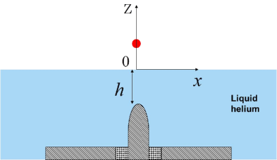
Figure 1: (Color online) A sketch of an electron floating on the surface of liquid helium and controlled by a micro-electrode Dykman .

As the electron emerges in the vacuum over the liquid helium surface, it will be attracted towards the surface by the image-attractive force. With a few angstroms of the surface, the electron encounters a strong repulsive barrier along the $z$-direction (arising from the Pauli exclusion principle), which prevents the electron from penetrating into the liquid helium. The potential well, formed by the sum of the image potential and the repulsive barrier, supports a series of bound electronic states which are very similar to those in the hydrogen atom. Mathematically, such a 1D hydrogen-atom-like potential takes the form Zhang

$$V(z)=\left\{\begin{aligned} -\frac{\Lambda e^{2}}{z},~{}~{}~{}~{}~{}~{}&z>0\\ V_{0},~{}~{}~{}~{}~{}~{}&z\leq 0\end{aligned}\right.$$ (1)

where $z$ is the coordinate of the electron perpendicular to the interface and $e$ the charge of the electron. The coefficient $\Lambda$ is $\Lambda\equiv(\epsilon-1)/[4(\epsilon+1)]\cong 0.0069$ with a helium dielectric constant of $\epsilon\cong 1.057$  Gordon . The height of the repulsive barrier $V_{0}$ has been measured to be approximately $1~{}\rm eV$ Woolf , which is a sufficiently-strong obstacle such that the electron cannot drop into the liquid helium. Therefore, the Hamiltonian of a single electron floating on the surface of liquid helium can be simply written as

$$\hat{H}=\frac{p^{2}}{2m}-\frac{\Lambda e^{2}}{z}.$$ (2)

By the usual finite difference method, we numerically solve the the relevant spectrum problem related to the Hamiltonian (2) and find that the ground state and the lower two excited state energies are $E_{0}=-0.65~{}\rm meV$, $E_{1}=-0.16~{}\rm meV$, $E_{2}=-0.072~{}\rm meV$ respectively. The qubit is encoded by the two lower states with the energy-splitting $\omega_{10}=(E_{1}-E_{0})/\hbar\sim 2\pi\times 117~{}\rm GHz$. The lower four states and their corresponding wavefunctions are shown in Fig. 2. Certainly, the energy-splittings of these bound states can be controlled by the Stark field applied normally to the surface Grimes .

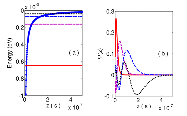
Figure 2: (Color online) The lower four bound states and their corresponding wave functions of a surface-state electron on liquid helium: (a) Lower four bound-state energy levels in the potential (solid blue line), and (b) The corresponding eigenfunctions. The red, dashed purple, dotted-dashed blue and dotted black lines denote the ground, the first excited, the second excited and the third excited states, respectively.

II.2 Rabi oscillations

The most popular approach to implement the population transfer between the selected qubit’s states is by using the Rabi oscillations, i.e., the population of one qubit’s state undergoes a sinusoidal variation. Here, the quantum transition between the qubit’s states is induced by applying a resonant driving field Bergmann . The Hamiltonian of the driven qubit reads

$$\hat{H}_{R}(t)=\frac{\hbar\omega_{0}}{2}\hat{\sigma}_{z}+R(t)\hbar\hat{\sigma}_{x},$$ (3)

with $\omega_{0}=\omega_{10}$ being the transition frequency of the qubit and $R(t)$ the controllable coupling between the qubit states; $\hat{\sigma}_{z}$ and $\hat{\sigma}_{x}$ are the Pauli operators, with $\hat{\sigma}_{x}=|0\rangle\langle 1|+|1\rangle\langle 0|$ and $\hat{\sigma}_{z}=|1\rangle\langle 1|-|0\rangle\langle 0|$. For the resonant driving field $E_{ac}=\varepsilon(t)\cos(\nu t)$, the induced coupling between the qubit’s states takes the form $R(t)=\Omega(t)\cos(\nu t)$, with $\nu=\omega_{0}$ and $\Omega(t)=e\varepsilon(t)z_{10}/\hbar$ being the Rabi frequency. Also, $\varepsilon(t)$ and $z_{10}=\langle 1|z|0\rangle$ are the amplitude of the applied pulse and the matrix element of the electric dipole moment respectively.

In the interaction picture defined by the unitary transformation $\hat{U}_{0}=\exp[-i\omega_{0}\hat{\sigma}_{z}t/2]$, Eq. (3) can be transformed to the form

$$\hat{H}_{\rm int}=\hat{U}_{0}^{\dagger}R(t)\hat{\sigma}_{x}\hat{U}_{0}=\frac{\Omega(t)}{2}\hbar\hat{\sigma}_{x}.$$ (4)

Formally, the time-evolution operator corresponding to this Hamiltonian reads

$$U(t) =\exp\left(-\frac{i}{\hbar}\int_{0}^{t}\hat{H}_{\rm int}(t^{\prime})dt^{\prime}\right)$$

$$=\cos(\frac{D(t)}{2})\rm I-i\sin(\frac{D(t)}{2})\hat{\sigma}_{x},$$ (5)

with $D(t)=\int_{0}^{t}\Omega(t^{\prime})dt^{\prime}$ is the area of the pulse and $\rm I$ an unit matrix. Obviously, if the qubit is initially prepared in the $|0\rangle$ state, then after a time $t$ the qubit will evolve into the $|1\rangle$ state with a probability $P(t)=[1-\cos D(t)]/2$. Therefore, in order to realize the complete inversion of the population, the applied pulse must be precisely designed as a $\pi$-pulse. Also, a precise “$\pi/2$-pulse” is required to prepare the superposition state $(|0\rangle-i|1\rangle)/\sqrt{2}$.

II.3 Precisely controlling durations for two-qubit gate

A significant progress in quantum computing is to achieve the single-qubit gate and the two-qubit gate. For the present system the implementation of the desired two-qubit gate is not easy, as the interbit coupling is always-on Dykmanf . Indeed, due to the always-on Coulomb interaction, the Hamiltonian of two nearest-neighbor electrons moving along the $z$ direction can be well approximated as

$$V_{c}(z_{1},z_{2})\approx\frac{e^{2}}{2d^{3}\cdot 4\pi\epsilon_{0}}(z_{1}^{2}+z_{2}^{2}-2z_{1}z_{2}).$$ (6)

The Coulomb interaction between the electrons not only affects the state-dependent shift of the energy of the neighbor electron but also allows the resonant energy transfer from one electron to the other Platzman . In the computational basis, the Hamiltonian of the system can be rewritten as

$$\hat{H}_{h}=\sum_{j=1,2}\frac{\hbar\omega_{j}^{0}}{2}\hat{\sigma}_{j}^{z}+V_{c}(z_{1},z_{2}),$$ (7)

with $\hat{\sigma}_{j}^{z}=\rvert 1_{j}\rangle\langle 1_{j}\lvert-\rvert 0_{j}\rangle\langle 0_{j}\lvert$, and

$$\hat{V}_{c}(z_{1},z_{2}) = \zeta_{1}^{z}\hat{\sigma}_{1}^{z}+\zeta_{2}^{z}\hat{\sigma}_{2}^{z}+\zeta_{1}^{x}\hat{\sigma}_{1}^{x}+\zeta_{2}^{x}\hat{\sigma}_{2}^{x}+\zeta_{12}^{zz}\hat{\sigma}_{1}^{z}\hat{\sigma}_{2}^{z}+\zeta_{12}^{xx}\hat{\sigma}_{1}^{x}\hat{\sigma}_{2}^{x}+\zeta_{12}^{zx}\hat{\sigma}_{1}^{z}\hat{\sigma}_{2}^{x}+\zeta_{12}^{xz}\hat{\sigma}_{1}^{x}\hat{\sigma}_{2}^{z}.$$ (8)

In the above, $\omega_{j}^{0}$ is the transition frequency of the lower two levels referring to the $j$th electron, $\hat{\sigma}_{j}^{x}=\hat{\sigma}_{j}^{+}+\hat{\sigma}_{j}^{-}$ with $\hat{\sigma}_{j}^{+}=\rvert 1_{j}\rangle\langle 0_{j}\lvert$, $\hat{\sigma}_{j}^{-}=\rvert 0_{j}\rangle\langle 1_{j}\lvert$; and

$$\left\{\begin{aligned} &\zeta_{1}^{z}=\frac{e^{2}}{16\pi\varepsilon_{0}d^{3}}(z_{1}^{00}+z_{1}^{11}-z_{2}^{00}-z_{2}^{11})(z_{1}^{11}-z_{1}^{00}),\\ &\zeta_{2}^{z}=\frac{e^{2}}{16\pi\varepsilon_{0}d^{3}}(z_{2}^{00}+z_{2}^{11}-z_{1}^{00}-z_{1}^{11})(z_{2}^{11}-z_{2}^{00}),\\ &\zeta_{1}^{x}=\frac{e^{2}}{8\pi\varepsilon_{0}d^{3}}(z_{1}^{00}+z_{1}^{11}-z_{2}^{00}-z_{2}^{11})z_{1}^{01},\\ &\zeta_{2}^{x}=\frac{e^{2}}{8\pi\varepsilon_{0}d^{3}}(z_{2}^{00}+z_{2}^{11}-z_{1}^{00}-z_{1}^{11})z_{2}^{01},\end{aligned}\right.$$

and

$$\left\{\begin{aligned} &\zeta_{12}^{zz}=\frac{-e^{2}}{16\pi\varepsilon_{0}d^{3}}(z_{1}^{11}-z_{1}^{00})(z_{2}^{11}-z_{2}^{00}),\\ &\zeta_{12}^{xx}=\frac{-e^{2}}{4\pi\varepsilon_{0}d^{3}}z_{1}^{01}z_{2}^{01},\\ &\zeta_{12}^{zx}=\frac{-e^{2}}{8\pi\varepsilon_{0}d^{3}}(z_{1}^{11}-z_{1}^{00})z_{2}^{01},\\ &\zeta_{12}^{xz}=\frac{-e^{2}}{8\pi\varepsilon_{0}d^{3}}(z_{2}^{11}-z_{2}^{00})z_{1}^{01}.\end{aligned}\right.$$

Here, $z_{j}^{11}$, $z_{j}^{00}$ and $z_{j}^{01}$ are the matrix elements $\langle 1_{j}\lvert z_{j}\rvert 1_{j}\rangle$, $\langle 0_{j}\lvert z_{j}\rvert 0_{j}\rangle$, and $\langle 1_{j}\lvert z_{j}\rvert 0_{j}\rangle$, respectively. In the interaction picture defined by the unitary $\hat{U}_{1}(t)=\exp{[(-i/\hbar)t\sum_{j=1,2}\lambda_{j}\hat{\sigma}_{j}^{z}]}$ with $\lambda_{j}=\hbar\omega_{j}/2+\zeta_{j}^{z}$, the Hamiltonian of the system becomes

$$\hat{H}_{I}= \zeta_{12}^{zz}\hat{\sigma}_{1}^{z}\hat{\sigma}_{2}^{z}+\sum_{j=1,2}\zeta_{j}^{x}\left(e^{2it\lambda_{j}/\hbar}\hat{\sigma}_{j}^{+}+e^{-2it\lambda_{j}/\hbar}\hat{\sigma}_{j}^{-}\right)$$

$$+ \zeta_{12}^{xx}\left[e^{2it(\lambda_{1}+\lambda_{2})/\hbar}\hat{\sigma}_{1}^{+}\hat{\sigma}_{2}^{+}+e^{2it(\lambda_{1}-\lambda_{2})/\hbar}\hat{\sigma}_{1}^{+}\hat{\sigma}_{2}^{-}\right.\left.+e^{-2it(\lambda_{1}-\lambda_{2})/\hbar}\hat{\sigma}_{1}^{-}\hat{\sigma}_{2}^{+}+e^{-2it(\lambda_{1}+\lambda_{2})/\hbar}\hat{\sigma}_{1}^{-}\hat{\sigma}_{2}^{-}\right]$$

$$+ \zeta_{12}^{zx}\left(e^{2it\lambda_{1}/\hbar}\hat{\sigma}_{1}^{z}\hat{\sigma}_{2}^{+}+e^{-2it\lambda_{2}/\hbar}\hat{\sigma}_{1}^{z}\hat{\sigma}_{2}^{-}\right)+\zeta_{12}^{xz}\left(e^{2it\lambda_{1}/\hbar}\hat{\sigma}_{1}^{+}\hat{\sigma}_{2}^{z}+e^{-2it\lambda_{1}/\hbar}\hat{\sigma}_{1}^{-}\hat{\sigma}_{2}^{z}\right).$$ (9)

Consequently, under the usual rotating-wave approximation, we have

$$\overline{H}_{I}=\zeta_{12}^{zz}\hat{\sigma}_{1}^{z}\hat{\sigma}_{2}^{z}+\zeta_{12}^{xx}(\hat{\sigma}_{1}^{+}\hat{\sigma}_{2}^{-}+\hat{\sigma}_{1}^{-}\hat{\sigma}_{2}^{+}).$$ (10)

In the above derivation, we have assumed that $\lambda_{1}=\lambda_{2}$ for simplicity. Obviously, the Hamiltonian (10) yields the following two-qubit evolution

$$\hat{U} =e^{-i\hat{H}_{I}t/\hbar}=\left(\begin{array}[]{cccc}e^{-i\phi}&0&0&0\\ 0&e^{i\phi}\cos{\xi}&-i\sin{\xi}&0\\ 0&-i\sin{\xi}&e^{i\phi}\cos{\xi}&0\\ 0&0&0&e^{-i\phi}\end{array}\right),$$ (15)

$\text{with}\,\xi=t\zeta_{12}^{xx}/\hbar,\,\,\phi=t\zeta_{12}^{zz}/\hbar$. This is a typical two-qubit i-SWAP gate. With such an universal gate, assisted by arbitrary rotations of single qubits, any quantum computing network could be constructed Lloyds . If the two-qubit system is prepared beforehand in a pure state $|01\rangle$ (or $|10\rangle$), then under the i-swap gate operation, the state will evolve to $\hat{U}|01\rangle=\exp{(i\phi)}\cos{\xi}|01\rangle-i\sin{\xi}|10\rangle$ (or $\hat{U}|10\rangle=\exp{(i\phi)}\cos{\xi}|10\rangle-i\sin{\xi}|01\rangle$). Again, the population inversion: $|01\rangle\longrightarrow|10\rangle$ (or   $|10\rangle\longrightarrow|01\rangle$) could be exactly implemented by setting the evolution time exactly at $t=\hbar\pi/(2\zeta_{12}^{xx})$.

In principle, quantum computation with surface-state electrons on liquid helium can be implemented with the above universal gates. However, for implementing these gates the evolution times of the system should be exactly set. Any deviation of the desired duration will decrease the fidelity of the expectable gate. In the followings sections, we will show that the above quantum gates could be implemented by using various evolution-time insensitive quantum operations whose durations are not required to be exactly set.

III Quantum computation with trapped electrons on helium by population passages I: adiabatic manipulations

III.1 The adiabatic population passage model: SCRAP

Usually, the general logic gates in quantum computation are realized by precisely designed resonant pulses. As it has been mentioned above, in order to perform a one-qubit gate with an electron floating on liquid helium, an exactly designed $\pi$-pulse should be applied. However, due to the various fluctuations and operational imperfections occuring in practice, it is not easy to precisely design the applied pulses with exact durations. Therefore, implementing quantum logic gates insensitive to evolution time is highly desirable in our context. In 2008, Wei et. al. Wei proposed such an approach by using the Stark-chirped rapid adiabatic passage (SCPAP) technique. In this approach the dynamical Stark shift, induced by the applied pulse, is utilized to produce the required detuning chirp(s) of the qubit(s), and the usual Rabi pulse is used to drive the quantum transition between the qubit’s states. Once the orders of the applied pulses are properly set, the population of one qubit’s states can be deterministically passaged to the other. As a consequence, the desired quantum gate is implemented.

The basic idea of the SCPAP is briefly reviewed as follows. Generally, the time-dependent Hamiltonian of the driven two-level system under the applied Stark-chirped and Rabi pulses, $\Omega(t)$ and $R(t)$, reads

$$\hat{H}_{1}(t)=\frac{\hbar\omega_{0}}{2}\hat{\sigma}_{z}+\hbar R(t)\hat{\sigma}_{x}+\hbar\Delta(t)\frac{\hat{\sigma}_{z}}{2}.$$ (16)

In the interaction picture, this Hamiltonian reduces to

$$\hat{H}_{1}^{\prime}(t) =\frac{\hbar}{2}\left(\begin{array}[]{cc}0&\Omega(t)\\ \Omega(t)&2\Delta(t)\end{array}\right)=\frac{\hbar\varepsilon(t)}{2}\left(\begin{array}[]{cc}0&\sin{2\theta(t)}\\ \sin{2\theta(t)}&2\cos{2\theta(t)}\end{array}\right),$$ (21)

with $\varepsilon(t)$$=$$\sqrt{\Delta^{2}(t)+\Omega^{2}(t)}$ and $\theta(t)$$=$$\arctan[\Omega(t)/\Delta(t)]/2$. By solving the instantaneous eigenvalue equation of the Hamiltonian (13), one obtains the eigenvalues: $\lambda_{\pm}=\hbar[\Delta(t)\pm\sqrt{\Delta^{2}(t)+\Omega^{2}(t)}]/2$, and the relevant eigenvectors:

$$|\lambda_{+}(t)\rangle=\sin\theta(t)|0\rangle+\cos\theta(t)|1\rangle,$$ (22)

$$|\lambda_{-}(t)\rangle=\cos\theta(t)|0\rangle-\sin\theta(t)|1\rangle.$$ (23)

If the rate of the change of the Hamiltonian is slow enough, the so-called adiabatic condition,

$$\eta=\frac{\left|\Omega(t)d\Delta(t)/dt-\Delta(t)d\Omega(t)/dt\right|}{2[\Delta^{2}(t)+\Omega^{2}(t)]^{3/2}}\ll 1$$ (24)

is satisfied, the system will stay at its instantaneous eigenstate. And, there is no transition between the two instantaneous eigenstates $|\lambda_{-}(t)\rangle$ and $|\lambda_{+}(t)\rangle$. This implies that the system exists two independent adiabatic passages defined by its two instantaneous eigenstates.

If the system is initially prepared at one of the adiabatic states, it stays at this state during the adiabatic evolution but the populations of a diabatic basis $|0\rangle$ and $|1\rangle$ could be changed. Therefore, if the order of the applied pulses is right, the population of one state can be completely passaged to that of another state. Certainly, the relative phase of the computational basis depends on the evolution time. But, such a relative phase shift gate, which is sufficiently produced by the Stark pulse, can be written as $\hat{U}_{p}(\varrho)=\exp{(i\varrho|1\rangle\langle 1|)}$ with $\eta=-\int_{t_{0}}^{t_{f}}\Delta(t^{\prime})dt^{\prime}$. This phase shift gate implies the evolution: $|0\rangle\rightarrow|0\rangle$ and $|1\rangle\rightarrow e^{i\varrho}|1\rangle$. Therefore, the applied stark pulse just changes the phase accumulation of the qubit state $|1\rangle$, but does not destroy the population distribution between the states $|0\rangle$ and $|1\rangle$.

Obviously, the above adiabatic passage could be used to implement the desired single-qubit quantum gates Wei ; Nie for quantum computing. Of course, if the population transfer between the qubit states is not partial (but not completely inversion), then the population can be controllably distributed at the qubit’s states. As a consequence, the relevant superposition of the states $|0\rangle$ and $|1\rangle$ can be obtained.

III.2 Adiabatical population passages for single-qubit gates

In the Sec. II, we have shown that $z$-directional motion of an electron, trapped on the surface of liquid helium, could be effectively treated as hydrogenic-like atom. Therefore, the two lower states, $|0\rangle$ and $|1\rangle$, could be utilized to encode a qubit for storing quantum information. In order to perform the single-qubit with such a surface-state electron by using the SCRAP introduced previously, we apply a resonant pump electric-field and a dc micro-pulse to the electrode for coupling the qubit’s states and inducing the desired Stark shifts, respectively. With these external drivings introduced, the Hamiltonian of a floating electron on the liquid helium can be written as

$$\hat{H}_{1}(t)=\hat{H}_{0}+\hat{H}^{\prime}(t),$$ (25)

with

$$\hat{H}_{0}=\frac{\hat{p}^{2}}{2m}-\frac{\Lambda e^{2}}{z}=\sum_{i=0,1,2}E_{i}|i\rangle\langle i|,$$ (26)

and

$$\hat{H}^{\prime}(t) =eE_{dc}(t)z+e\xi(t)z\cos{w_{0}t}$$

$$=\left[eE_{dc}(t)+e\xi(t)\cos{w_{0}t}\right]\sum_{i,j=0,1,2}z_{ij}|i\rangle\langle j|,$$ (27)

where $z_{ij}=\langle i|z|j\rangle$ and $z_{ij}=z_{ji}$. The potential induced by the pump pulse is $V_{\rm pump}(t)=\xi(t)\cos{\omega_{0}t}$, where $\omega_{0}$ is the splitting frequency of the two lower state and $\xi(t)$ denotes intensity of the pump pulse. And $E_{dc}(t)$ leading to Stark shift of the energy levels is induced by the applying a $dc$-electric field to the electrode beneath the helium surface. Of course, the field induced by the electrode will both affect parallel and vertical motion of the electron to the surface. However, the parallel motion is just a harmonic oscillator and the oscillation frequency ($20~{}\rm GHz$) is sufficiently weak, and thus can be effectively neglected ( compared with the transition frequency of the qubit: $\omega_{0}=2\pi\times 117~{}\rm GHz$). Actually, the two pulses applied to implement the qubit operation can both generate the Stark shifts and also couple the two states of the qubit. However, in the interaction picture and under the usual rotating-wave approximation, the Stark shift induced by the pump pulse can be effectively ignored (compared with that induced by the dc pulse), and also that coupling induced by the dc pulse is negligible (compared with that induced by the applied pump pulse).

Under the unitary transformation $\hat{U}_{0}(t)=\exp{(-i\hat{H}_{0}t/\hbar)}$, defined in the interaction picture, the Hamiltonian (25) can be rewritten as

$$\hat{H}_{i}(t)=\left(\begin{array}[]{ccc}0&\kappa z_{01}&0\\ \kappa z_{10}&eE_{dc}(t)(z_{11}-z_{00})&0\\ 0&0,&eE_{dc}(t)(z_{22}-z_{00})\end{array}\right),$$ (31)

where $\kappa=e\xi(t)/2$, $z_{00}=0.0115~{}\rm\mu m$, $z_{11}=0.0461~{}\rm\mu m$, $z_{22}=0.1038~{}\rm\mu m$, $z_{01}=z_{10}=-0.0043~{}\rm\mu m$, and $z_{12}=z_{21}=0.0142~{}\rm\mu m$.

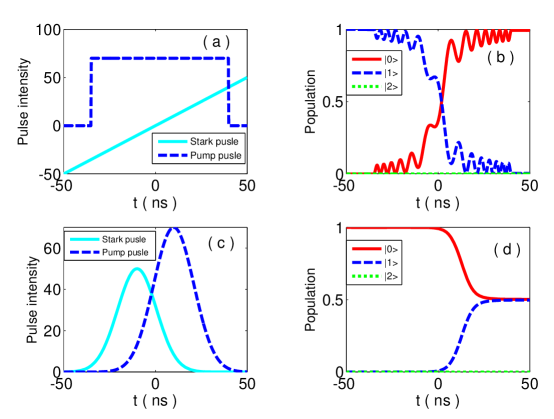
Figure 3: (Color online) SCRAP-based population evolution of the lower three states of the surface-state electron. The applied pulse sequences are shown in (a), (c); and the corresponding population transitions are shown in (b), (d), respectively. In (a) the two pulses are designed with the linear forms $E_{dc}(t)=1\times 10^{9}t~{}\rm V/m$ and $\xi(t)=70~{}\rm V/m~{}(-35~{}\rm ns\leq t\leq 40~{}\rm ns,~{}\text{else where}~{}\xi(t)=0~{}\rm V/m)$. With this pulse sequence and $\beta=0.13$, the electron initially prepared in the state $|1\rangle$ completely passages to the state $|0\rangle$, see, Fig. 3(b). It is clearly seen that the population leaking to the upper state $|2\rangle$ is sufficient small that can be safely neglected. In (c) two Gaussian, $E_{dc}(t)=50\exp{[-(t+10)^{2}/(15)^{2}]}~{}\rm V/m$ and $\xi(t)=70\exp{[-(t-10)^{2}/(15.5)^{2}]}~{}\rm V/m$ with $\beta=0.09$, are designed to generate the superposition state $(|0\rangle+|1\rangle)/\sqrt{2}$ from the initial state $|0\rangle$. The relevant population changes are shown in Fig. 3(d). It is also shown that during such a SCRAP, the population of the state $|2\rangle$ is always sufficiently small and consequently any leakage of the qubit(s) can be neglected.

Fig. 3 shows the time evolutions of the populations in the lower three states of surface-state electron during the designed SCRARs. One can see that the usual $\hat{\sigma}_{x}$-rotation operation and the Hadamard-like single-qubit gate could be implemented adiabatically. Specifically, when the pulses with the form dipicted in Fig. 3(a) are applied to the electrode, the electron initially prepared in the state $|1\rangle$ can be completely passaged to the state $|0\rangle$ along the adiabatic path $|\lambda_{-}(t)\rangle$. Conversely, if the electron initially prepared in the ground state $|0\rangle$, then it is completely transferred to the first excited state $|1\rangle$ along the adiabatic paths $|\lambda_{+}(t)\rangle$. On the other hand, in order to utilize the SCRAP technique to implement the Hadamard-like gate, we use two Gaussian pulses (rather than the above linear pulses). The pulse sequence is indicated in Fig. 3(c), wherein the Stark pulse is applied firstly and later the pump pulse is applied, but the Stark pulse switches off prior to the pump pulse. With such a pulse sequence, the initial evolution condition $\theta(t_{0})=\pi$ and the final one $\theta(t_{f})=\pi/4$ are both satisfied, thus the initial state $|0\rangle$ will evolve to the superposition state $(|0\rangle+|1\rangle)/\sqrt{2}$ along the adiabatic path $|\lambda_{+}(t)\rangle$, or to the state $(|0\rangle-|1\rangle)/\sqrt{2}$ from the initial state $|1\rangle$ via the population passage along the path $|\lambda_{-}(t)\rangle$. Note again that, all these operations require the orders of the applied pulses be properly designed, but not the pulse durations. Intuitively, the electron may populate to the higher state $|2\rangle$ as the external pulse applied. However, as it is shown in Fig. 3(b), the probability of the unwanted transition between the states $|1\rangle$ and $|2\rangle$ is sufficiently small and thus could be ignored.

It is emphasized that, the designed SCRAPs are really insensitive to the durations of the pulses, as long as they are longer than, e.g., $\sim 100\,n$s. Also, our numerical solution confirms that the desired adiabatic population transfers are still sufficiently fast, e.g., within the time interval: $0.1~{}\rm\mu s$, which is significantly shorter than the decoherence time $(\sim 0.1~{}\rm ms$ Platzman ) of the system.

III.3 Adiabatical population passages for two-qubit gates

By precisely controlling the duration of the microwave pulse applied via the patterned electrode (beneath the surface liquid helium), it was shown Platzman ; Dykmanf ; LEA that a crucial two-qubit gate, i.e., the i-SWAP one, can be realized. In this subsection, we show that this rigorous requirement of precisely designing the duration of the applied pulse can be relaxed, and the same two-qubit gate can be effectively realized via evolution-time insensitive population passages.

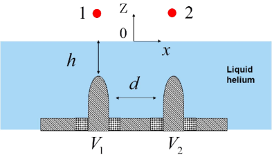
Figure 4: (Color online) The geometry of a two-qubit system with two electrons above the liquid helium and the micro-electrode. The electrodes are designed to confine the electrons and induce the Stark shifts to the electronic states. $V_{1}$ and $V_{2}$ are the control potentials of the two electrons, and $d\approx h=0.5~{}\rm\mu m$.

We consider the two electrons (portrayed in Fig. 4) trapped in the spatially-separated potentials $V_{1}$ and $V_{2}$, respectively. Suppose that the electrons have been cooled to sufficiently-low temperature and their surface-states are safely populated at the ground state (if there is not any driving pulse). Also, the electric fields applied to the electrons along the z-axis are different (i.e., $\bar{E}_{1}\neq\bar{E}_{2}$) to make the electrons be non-resonant. To realize the desired SCRAP, we now fix the electric field applied to the first qubit and change that applied to the second one. The Hamiltonian describing the driven two-electron on the liquid helium can be written as

$$\hat{H}_{\rm total} =\sum_{i=1,2}\hat{H}_{0}^{(i)}(z_{i})+\hat{H}_{\rm int}(z_{1},z_{2})+\hat{H}_{\rm stark}^{(2)}(t),$$

with

$$\hat{H}_{0}^{(i)} =\frac{p_{i}^{2}}{2m}-\frac{\Lambda e^{2}}{z_{i}}+ez_{i}\bar{E}_{i}+\frac{e\bar{E}_{j}z_{i}}{\sqrt{8}},\,\,i\neq j=1,2,$$

$$\hat{H}_{\rm int} =\frac{e^{2}}{4\pi\epsilon_{0}}\times\frac{z_{1}^{2}+z_{2}^{2}-2z_{1}z_{2}}{2d^{3}},$$

and

$$\hat{H}_{\rm stark}^{(2)}(t)=\left(eE_{dc}^{(2)}(t)z_{2}+\frac{eE_{dc}^{(2)}(t)z_{1}}{\sqrt{8}}\right).$$

Above, $\hat{H}_{0}^{(i)}$ is the non-perturbed Hamiltonian of each electron, $\hat{H}_{\rm int}$ represents the Coulomb interaction between the electrons (along the z-axis direction), and $\hat{H}^{(2)}_{\rm stark}(t)$ is the chirp term of the second electron implemented by applying a $dc$ electric field $E_{dc}^{(2)}$ with changeable amplitude. Since the energy-splitting between the ground state and the first excited state is larger than the one between the first excited state and the second excited state, the unwanted non-resonant transition between the states $|1\rangle$ and $|2\rangle$ can be safely neglected during the operations applied to the qubits. As a consequence, in the computational basis the above total Hamiltonian $\hat{H}_{\rm total}$ can be rewritten as

$$\hat{H}_{\rm Int}(t)=\left(\begin{array}[]{cccc}\Delta_{1}&0&0&0\\ 0&\Delta_{2}&-2\alpha z_{1}^{01}z_{2}^{10}e^{-i\omega t}&0\\ 0&-2\alpha z_{1}^{10}z_{2}^{01}e^{i\omega t}&\Delta_{3}&0\\ 0&0&0&\Delta_{4}\end{array}\right),$$ (36)

where $\alpha=e^{2}/(2d^{3}\times 4\pi\epsilon_{0}),\,\omega=\omega_{10}^{(1)}-\omega_{10}^{(2)}$,   $\omega_{10}^{(i)}=(E_{1}^{(i)}-E_{0}^{(i)})/\hbar$, and

$$\Delta_{1}= \alpha[(z_{1}^{00})^{2}+z_{1}^{01}z_{1}^{10}+(z_{2}^{00})^{2}+z_{2}^{01}z_{2}^{10}-2z_{1}^{00}z_{2}^{00}]+eE_{dc}^{(2)}z_{2}^{00}+\frac{eE_{dc}^{(2)}}{\sqrt{8}}z_{1}^{00},$$

$$\Delta_{2}= \alpha[(z_{1}^{00})^{2}+z_{1}^{01}z_{1}^{10}+(z_{2}^{11})^{2}+z_{2}^{10}z_{2}^{01}-2z_{1}^{00}z_{2}^{11}]+eE_{dc}^{(2)}z_{2}^{11}+\frac{eE_{dc}^{(2)}}{\sqrt{8}}z_{1}^{00},$$

and

$$\Delta_{3}= \alpha[(z_{1}^{11})^{2}+z_{1}^{10}z_{1}^{01}+(z_{2}^{00})^{2}+z_{2}^{01}z_{2}^{10}-2z_{1}^{11}z_{2}^{00}]+eE_{dc}^{(2)}z_{2}^{00}+\frac{eE_{dc}^{(2)}}{\sqrt{8}}z_{1}^{11},$$

$$\Delta_{4}= \alpha[(z_{1}^{11})^{2}+z_{1}^{10}z_{1}^{01}+(z_{2}^{11})^{2}+z_{2}^{10}z_{2}^{01}-2z_{1}^{11}z_{2}^{11}]+eE_{dc}^{(2)}z_{2}^{11}+\frac{eE_{dc}^{(2)}}{\sqrt{8}}z_{1}^{11},$$

with $z_{ij}=\langle i|z|j\rangle$ and $z_{ij}=z_{ji}$.

It is obviously seen from the Hamiltonian (36) that the two-qubit state $|00\rangle$ (or $|11\rangle$) forms an invariant subspace, i.e., if the two-qubit is initially prepared in the state $|00\rangle$ (or $|11\rangle$), then it always populates in such a state. On the otherhand, the states $|01\rangle$ and $|10\rangle$ together form an invariant subspace, i.e., only the transition between these states is allowable, and in this invariant subspace the Hamiltonian of the system reduces to

$$\hat{H}_{\rm sub}(t)=\left(\begin{array}[]{cc}0&-2\alpha z_{1}^{01}z_{2}^{10}e^{-i\omega t}\\ -2\alpha z_{1}^{10}z_{2}^{01}e^{i\omega t}&\Delta_{3}-\Delta_{2}\end{array}\right),$$ (39)

Fig. 5(a) exhibits how the population of one two-qubit state (e.g., $|01\rangle$) passages to another one (e.g., $|10\rangle$) along the relevant adiabatic path. Here, the parameters used in the numerical simulations are: $z_{1}^{00}=0.0115~{}\rm\mu m$, $z_{1}^{11}=0.0457~{}\rm\mu m$, $z_{1}^{01}=z_{1}^{10}=-0.0043~{}\rm\mu m$, $z_{2}^{00}=0.0115~{}\rm\mu m$, $z_{2}^{11}=0.0458~{}\rm\mu m$, $z_{2}^{01}=z_{2}^{10}=-0.0043~{}\rm\mu m$, and $E_{dc}^{(2)}(t)=\gamma t$ with $\gamma=1\times 10^{9}\,V/(m\times s)$. Fig. 5(b) clearly shows that the requirement of accurately designing the interaction time between the qubits is removed. If the electrons are initially prepared in the state $|01\rangle$, then the population is adiabatically changed to the state $|10\rangle$ along the red-line path in Fig. 5(a). Once the duration of the driving pulse is set as $\tau_{a}>400$ns here, the population is transferred completely.

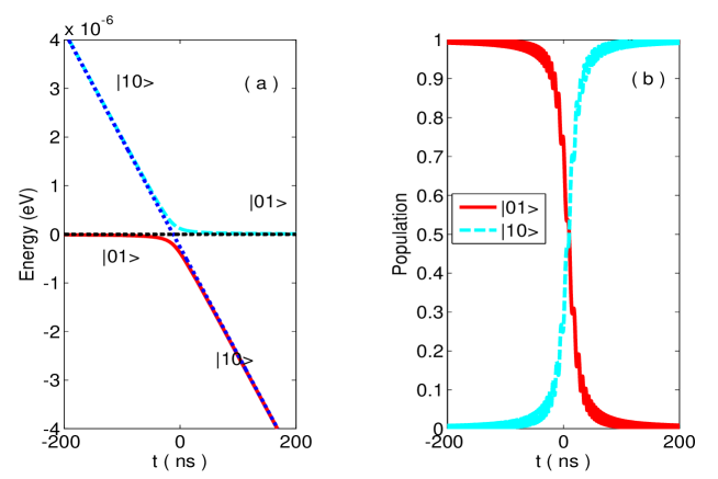
Figure 5: (Color online) Population passages between the two two-qubit states under the SCRAP. (a) Adiabatic passages, and (b) the population transferred from the state $|01\rangle$ to the state $|10\rangle$. The adiabatic parameter is $\beta=0.1$.

IV Quantum computation with trapped electrons on helium by population passages II: non-adiabatic manipulations

IV.1 Evolution operator for a driven two-level system

In the above SCRAP, the implementations of the usual quantum gates are based on various adiabatic process along the independent paths. Generally, these passages require that the evolutions of the driven system should be significantly slow such that the adiabatic conditions could be satisfied. However, the required adiabatic condition is essentially limited by the defined decoherence time. Therefore, relaxing the adiabatic condition required in the above SCRAP technique is practically important for the realistic quantum gates.

In order to implement the quantum computation beyond the adiabatic limit, in this section we introduce a series of non-adiabatic passages of the qubits’ populations. To this end, we begin with a generic time-driven two-level system Xian

$$\hat{H}(t)=[A(t)-\frac{1}{2}\hbar\dot{\omega}(t)]\hat{\sigma}_{z}+B(t)\hat{\sigma}_{x},$$ (40)

where $A(t)$, $B(t)$ and $\omega(t)$ are the controllable real parameters. The dynamics of such a generic time-dependent system is described by the Schr$\rm\ddot{o}$dinger equation

$$i\hbar\frac{\partial}{\partial t}|\Psi(t)\rangle=\hat{H}(t)|\Psi(t)\rangle.$$ (41)

Suppose that the system is initially prepared in its ground state, i.e., $|\Psi(t_{0})\rangle=|0\rangle$, then the state after the evolution time $t$ reads $|\Psi(t)\rangle=\hat{U}(t)|\Psi(t_{0})\rangle$ with $\hat{U}(t)$ being the evolution operator. It obeys the follow equation

$$i\hbar\frac{\partial}{\partial t}\hat{U}(t)=\hat{H}(t)\hat{U}(t),$$ (42)

with the formal solution Ya ,

$$\hat{U}(t)= \left(\begin{array}[]{cc}\cos[\alpha(t)]&i\sin[\alpha(t)]\\ i\sin[\alpha(t)]&\cos[\alpha(t)]\end{array}\right)\times\left(\begin{array}[]{cc}e^{i\gamma(t)}&0\\ 0&e^{-i\gamma(t)}\end{array}\right)\times\left(\begin{array}[]{cc}\cos[\beta(t)]&\sin[\beta(t)]\\ -\sin[\beta(t)]&\cos[\beta(t)]\end{array}\right).$$ (49)

Here, the initial condition $\hat{U}(0)=1$ implies that, $\alpha(0)=\beta(0)=\gamma(0)=0$, and the relevant time-dependent parameters: $\alpha(t),\,\beta(t),$ and $\gamma(t)$, are determined by the following differential equations:

$$\left\{\begin{aligned} \dot{\alpha}&=-[A(t)-\frac{1}{2}\dot{\omega}(t)]\cos[2\alpha(t)]\tan[2\beta(t)]-B(t),\\ \dot{\beta}&=[A(t)-\frac{1}{2}\dot{\omega}(t)]\sin[2\alpha(t)],\\ \dot{\gamma}&=-[A(t)-\frac{1}{2}\dot{\omega}(t)]\frac{\cos[2\alpha(t)]}{\cos[2\beta(t)]}.\end{aligned}\right.$$ (50)

Once Eq. (50) is solved, wave-function of the system at any time can be obtained.

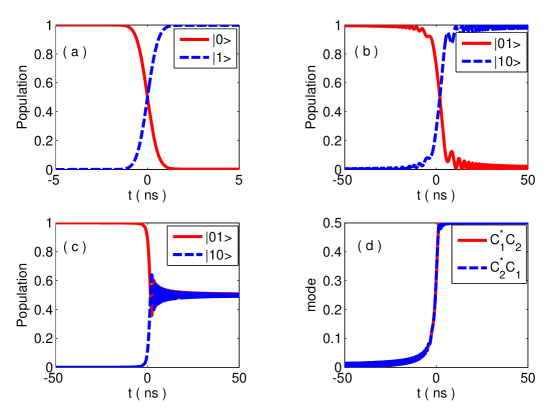
Figure 6: (Color online) Non-adiabatic implementation of the usual quantum gates and the preparation of Bell state. The $\hat{\sigma}_{x}$-rotating gate shown in (a) is achievable by using the Gaussian pulses $E_{dc}^{\prime}(t)=10\exp{[-t^{2}/(1\times-10)^{2}]}~{}\rm V/m$ and $E_{ac}^{\prime}(t)=270\exp{[-t^{2}/(1\times-9)^{2}]}~{}\rm V/m$. The $i$-swap gate is achieved by introducing a linear $dc$ micro-field to the second electron: $E_{dc}^{\prime(2)}(t)=6\times 10^{9}t~{}\rm V/m$, shown in (b). In (c) the equivalent-probability superposition of the states $|01\rangle$ and $|10\rangle$ is given, after a fast population passage process by applying the pulse $E_{dc}^{\prime(2)}(t)=28\times 10^{9}t~{}\rm V/m$. In (d) the non-zero real parts of the non-diagonal elements of the density matrix of the generated superposed state are shown. This confirms that the system is really prepared in a coherent superposition state (rather than the mixed one).

IV.2 Non-adiabatical passage for the single-qubit gate

The Hamiltonian describing the present fast-driven single qubit can be expressed as

$$\hat{H}_{1}(t)=\frac{eE_{dc}^{\prime}(t)(z_{11}-z_{00})}{2}\hat{\sigma}_{z}+\frac{e\xi^{\prime}(t)z_{01}}{2}\hat{\sigma}_{x},$$ (51)

where $E_{dc}^{\prime}(t)$ is the dc micro-pulse (which induces the desired stark shift) and $\xi^{\prime}(t)$ is the amplitude of the resonant pump electric-field (which is used to couple the qubit’s states). By Runge-Kutta method we can numerically solve the relevant Eq. (50) and then exactly determine the time-evolution operator $\hat{U}(t)$. Consequently, if the qubit begins with the ground state $|0\rangle$ (the excited state $|1\rangle$), then after the time $t$, the probability of the population being transferred completely to the excited state $|1\rangle$ (the ground state $|0\rangle$) is

$$P_{1}(t) =1-|\langle 0|\hat{U}(t)|0\rangle|^{2}$$

$$=1-\left|\cos[\alpha(t)]\cos[\beta(t)]-i\sin[\alpha(t)]\sin[\beta(t)]\right|^{2},$$ (52)

or

$$P_{0}(t) =1-|\langle 1|\hat{U}(t)|1\rangle|^{2}$$

$$=1-\left|i\sin[\alpha(t)]\cos[\beta(t)]-\cos[\alpha(t)]\sin[\beta(t)]\right|^{2}.$$ (53)

Fig. 6(a) shows that the $\hat{\sigma}_{x}$-rotation gate is implemented by introducing two Gaussian pulses. Note that the Gaussian pulses introduced here go against the adiabatic condition (24) (i.e., the adiabatic parameter is $\beta=0.7$), and thus the population passages for implementing the $\hat{\sigma}_{x}$-rotation gate are non-adiabatic. Indeed, in the adiabatic basis: $|\lambda_{-}(t)\rangle$ and $|\lambda_{+}(t)\rangle$, the Hamiltonian of the present driven qubit can be rewritten as

$$\hat{H}_{nad}=\left(\begin{array}[]{cc}\lambda_{-}(t)&-id\theta(t)/dt\\ id\theta(t)/dt&\lambda_{+}(t)\end{array}\right).$$ (56)

Obviously, the non-diagonal elements are not zero, and thus the populations of the two adiabatic states ($|\lambda_{-}(t)\rangle$ and $|\lambda_{+}(t)\rangle$) are oscillating before the desired passages finish.

IV.3 Non-adiabatical passage for the two-qubit gate

To implement the two-qubit i-swap gate, we need to achieve the $\pi/2$-rotation between the states $|01\rangle$ and $|10\rangle$. The dynamics for realizing such a driving is

$$\hat{H}_{\rm sub}^{\prime}(t)=\left(\begin{array}[]{cc}\Delta^{\prime}_{2}&-2\alpha z_{1}^{01}z_{2}^{10}e^{-i\omega t}\\ -2\alpha z_{1}^{10}z_{2}^{01}e^{i\omega t}&\Delta^{\prime}_{3}\end{array}\right),$$ (59)

which is similar to that in Eq. (40) for the previously adiabatic passage. Here,

$$\Delta_{2}^{\prime}= \alpha[(z_{1}^{00})^{2}+z_{1}^{01}z_{1}^{10}+(z_{2}^{11})^{2}+z_{2}^{10}z_{2}^{01}-2z_{1}^{00}z_{2}^{11}]+eE_{dc}^{\prime(2)}z_{2}^{11}+\frac{eE_{dc}^{\prime(2)}}{\sqrt{8}}z_{1}^{00},$$

$$\Delta_{3}^{\prime}= \alpha[(z_{1}^{11})^{2}+z_{1}^{10}z_{1}^{01}+(z_{2}^{00})^{2}+z_{2}^{01}z_{2}^{10}-2z_{1}^{11}z_{2}^{00}]+eE_{dc}^{\prime(2)}z_{2}^{00}+\frac{eE_{dc}^{\prime(2)}}{\sqrt{8}}z_{1}^{11}.$$

The above Hamiltonian can be further simplified as

$$\hat{H}_{2}= \left(\frac{\Delta_{2}^{\prime}-\Delta_{3}^{\prime}}{2}-\frac{1}{2}\hbar\omega\right)(|01\rangle\langle 01|-|10\rangle\langle 10|)-2\alpha(z_{1}^{01}z_{2}^{10}|01\rangle\langle 10|+|10\rangle\langle 01|).$$ (60)

Again, we can numerically solve the evolution operator corresponding this Hamiltonian and then investigate the population transfers between the states $|01\rangle$ and $|10\rangle$. Fig. 6(b) shows clearly that, if the proper amplitude-adjustable $dc$ micro-field is applied to the second electron, the desired $i$-swap gate can be implemented non-adiabatically. The relevant adiabatic parameter is $\beta=0.5$, and the time interval for realizing such a gate is shortened to $\tau_{\rm na}>100$ ns (which is significantly shorter than $\tau_{a}>400$ns for the precious adiabatic passage.)

Furthermore, by designing the proper non-adiabatic passage the two-qubit Bell state (the maximal entangled one of the two-qubit system) can be fast generated deterministically. In fact, our numerical results shown in Fig. 6(c) indicates that, an equivalent-probability superposition of the states $|01\rangle$ and $|10\rangle)$ is deterministically generated after the non-adiabatic passages of the populations (with the adiabatic parameter $\beta=2.15$). Also, we can prove that such a superposition is coherent. Indeed, in the subspace spanned by the states $|01\rangle$ and $|01\rangle$, the evolution of the system can be generally expressed as

$$\psi_{\rm sub}(t)=C_{1}(t)|01\rangle+C_{2}(t)|10\rangle,$$ (61)

where $C_{1}(t)$ and $C_{2}(t)$ are the probabilistic amplitudes. Thus, the reduced density matrix in this subspace reads

$$\rho_{\rm sub}(t)=\left(\begin{array}[]{cc}|C_{1}(t)|^{2}&C_{1}^{*}C_{2}(t)\\ C_{2}^{*}(t)C_{1}(t)&|C_{2}(t)|^{2}\end{array}\right).$$ (64)

Suppose that the system is initially prepared in the state $|01\rangle$, then the corresponding probability amplitudes (at any time $t$) are $C_{1}(t)=\{\cos[\alpha(t)]\cos[\beta(t)]-i\sin[\alpha(t)]\sin[\beta(t)]\}\exp{(i\gamma)}$ and $C_{2}(t)=\{i\sin[\alpha(t)]\cos[\beta(t)]-\cos[\alpha(t)]\sin[\beta(t)]\}\exp{(i\gamma)}$. Fig. 6(d) shows that the real parts of the parameters $C_{1}^{*}(t)C_{2}(t)$ and $C_{2}^{*}(t)C_{1}(t)$ are really not zero. This indicates that the superposition of the states $|01\rangle$ and $|10\rangle$ (deterministically generated by the above non-adiabatic population passages) is coherent.

V Conclusions and Discussions

In summary, we have investigated how to implement the single- and two-qubit gates by using the population passage technique. We have shown that the deterministic populations transfers between the selected quantum states can be achieved by applying either adiabatic or non-adiabatic pulses to the qubit(s). It is emphasized that, differing from the approach to implement the quantum gates by using precisely-designed pulses with exact durations, the quantum gates implemented by the present population transfers are insensitive to the durations of the applied pulses, whatever the relevant evolutions are adiabatic or not. For the adiabatic passages the driven qubit(s) evolves along the induced adiabatic paths. While, under the non-adiabatic drivings the desired quantum gates could still be deterministically implemented within the significantly-short time. This is important to robustly overcome the decoherence existed in the realistic systems. With the proposed non-adiabatic passage technique, we have also shown that the Bell state could be deterministically generated.

Our generic proposal is demonstrated specifically with the surface-state electrons on the liquid helium Platzman . This system possesses several important advantageous features, e.g., it could be conveniently manipulated by the electrodes beneath the helium surface, the system could be easily fabricated and integrated, and the qubit(s) can be simply addressed and read out, etc.. Particularly, the surface-state electrons on the liquid helium possess the sufficiently-long coherence times. For example, it can reach to $0.1~{}\rm ms$ at $10~{}\rm mK$. While, the durations of the proposed adiabatic passages to implemented the desired single-qubit and two-qubit operations are just $100\rm ns$ and $400\rm ns$, respectively. Furthermore, if the non-adiabatic passages are applied, durations of $10\rm ns$ and $100\rm ns$ are enough to realize the single-qubit and two-qubit gates, respectively. Therefore, the feasibility of our proposal can be tested relatively-easily with the surface-state electrons, although it is still limited Platzman by the experimental challenge of single-electron readouts.

References

- (1) S. Lloyd, Science 261, 5128 (1993).
- (2) P. W. Shor, Proceedings of the 35th Annual Symposium on Foundations of Computer Science (IEEE Computer Press,Los Alamitos, 1994), p. 124.
- (3) L. K. Grover, Phys. Rev. Lett. 79, 325 (1997).
- (4) Peter W. Shor, Phys. Rev. A 52, R2493 (1995).
- (5) M. Fleischhauer, R. Unanyan, B. W. Shore and K. Bergmann, Phys. Rev. A 52, R2493 (1995).
- (6) B. W. Shore, K. Bergmann, A. Kuhn, S. Schiemann and J.Oreg, Phys. Rev. A 45, 5297 (1992).
- (7) K. Bergmann, H. Theuer and B. W. Shore, Rev. Mod. Phys. 70, 1003 (1998).
- (8) T. Rickes, L. P. Yatsenko, S. Steuerwald, T. Hlfmann, B. W. Shore, N. V. Vitanov, and K. Bergmann, J. Chem. Phys. 113, 534 (2000).
- (9) A. A. Rangelov, N. V. Vitanov, L. P. Yatsenko, B. W. Shore, T. Halfmann and K. Bergmann, Phys. Rev. A 72, 053403 (2005).
- (10) L. P. Yatsenko, N. V. Vitanov, B. W. Shore, T. Rickes, K. Bergmann, Opt. Commun. 204, 413 (2002).
- (11) P. M. Platzman and M. I. Dykman, Science 284, 1967 (1999).
- (12) S. A. Lyon, Phys. Rev. A 74, 052338 (2006).
- (13) M. I. Dykman, P. M. Platzman, and P. Seddighrad, Phys. Rev. B 67, 155402 (2003).
- (14) S. Mostme and R. SCHtzhold, Phys. Rev. Lett. 101, 220501 (2008).
- (15) E. Collin, W. Bailey, P. G. Frayne, K. Harrabi, M. J. Lea and G. Papageorgin, Phys. Rev. Lett. 89, 245301 (2002).
- (16) Miao Zhang, H. Y. Jia and L. F. Wei, Phys. Rev. A 80, 055801 (2009).
- (17) Gordon F. Sabille, John M. Goodkind, and P. M. Platzman, Phys. Rev. Lett. 70, 1517 (1993).
- (18) M. A. Woolf, G. W. Rayfield, Phys. Rev. Lett. 15, 235 (1965).
- (19) C. C. Grimes, T. R. Brown, Michael L. Burns and C. L. Zipfel, Phys. Rev. B 13, 140 (1976).
- (20) M.I. Dykman and P.M. Platzman, Fortschr. Phys. 48, 1095 (2000).
- (21) L. F. Wei, J. R. Johansson, L. X. Cen, S. Ashhab, and Franco Nori, Phys. Rev. Lett. 100, 113601 (2008).
- (22) W. Nie, J. S. Huang, X. Shi, and L. F. Wei, Phys. Rev. B 82, 032319 (2010).
- (23) M.J. Lea, P.G. Frayne, Yu. Mukharsky, Fortschr. Phys. 48, 1109 (2000).
- (24) Xian-Geng Zhao, Phys. Lett. A 181, 425 (1993).
- (25) Ya-Feng Cao, Lian-Fu Wei and Bang-Pin Hou, Phys. Lett. A 374, 2281 (2010).