4th February, 2013

Summary

We develop algorithms for performing semiparametric regression analysis in real time, with data processed as it is collected and made immediately available via modern telecommunications technologies. Our definition of semiparametric regression is quite broad and includes, as special cases, generalized linear mixed models, generalized additive models, geostatistical models, wavelet nonparametric regression models and their various combinations. Fast updating of regression fits is achieved by couching semiparametric regression into a Bayesian hierarchical model or, equivalently, graphical model framework and employing online mean field variational ideas. An internet site attached to this article, realtime-semiparametric-regression.net, illustrates the methodology for continually arriving stock market, real estate and airline data. Flexible real-time analyses, based on increasingly ubiquitous streaming data sources stand to benefit.

Keywords: Approximate Bayesian inference; Generalized additive models; Mean field variational Bayes; Mixed models; Online variational Bayes; Penalized splines; Wavelets.

1 Introduction

Ongoing technological advancements mean that data are being collected and made available for inference with rapidly increasing volume and speed. There are numerous examples of this explosion of data, but two that have established connections with semiparametric regression, our focus in this article, are Internet auction analysis (e.g. Jank & Shmueli, 2007) and real-time spatial epidemiology (e.g. Kaimi & Diggle, 2011).

Semiparametric regression refers to a large class of regression models that provide for non-linear predictor effects using spline and wavelet basis functions, as well as dependencies arising in grouped data such as within-subject correlation. An arsenal of both frequentist and Bayesian fitting and inference procedures now exist. Recent overviews are contained in Ruppert, Wand & Carroll (2009) and Wand & Ormerod (2011).

Virtually all semiparametric regression methodology proposed to date assume that the data are processed in batch; that is, all at the same time. Summaries such as function estimates, confidence intervals and posterior density functions are then outputted. Downsides to batch processing include the requirement that statistical analysis wait until an entire data set has been assembled and, sometimes, the necessity of storing the entire data set in memory. In the online case, the procedure updates as each new data point (or subset of data points) is obtained. Online updates use only the new data and summary statistics from previous iterations rather than the full set of available data. A particular advantage of online processing is that summaries, such as those just mentioned, are updated throughout the data collection process and therefore are available immediately upon demand. Online processing also has the advantage of not requiring storage of potentially very large data-sets.

While a number of batch procedures exist for performing semiparametric regression, we focus on a particular methodology here due to the ease of adapting it to the online framework as well as its wide range of applicability. Consider single predictor nonparametric regression, a special case of semiparametric regression with a long history and large literature. Fully automatic nonparametric regression batch procedures include: (a) local linear kernel smoother with cross-validation bandwidth selection, (b) local linear kernel smoother with direct plug-in bandwidth selection, (c) frequentist low-rank smoothing spline with restricted maximum likelihood smoothing parameter selection, (d) Bayesian low-rank smoothing spline with Markov chain Monte Carlo approximate inference and (e) Bayesian low-rank smoothing spline with mean field variational Bayesian (MFVB) approximate inference. Details of (a) are in Härdle (1990), details of (b) are in Wand & Jones (1995), whilst (c) and (d) are described in Ruppert, Wand & Carroll (2003). Section 2.7 of Wand & Ormerod (2011) explains (e). Approaches (a)–(d) are more established, but none have a viable online modification. However, (e) is relatively easy to modify for this purpose.

Another advantage of the Bayesian low-rank smoothing spline approach to nonparametric regression is its extendibility. As explained in Wand (2009), couching semiparametric regression in a graphical models framework permits arbitrarily sophisticated models to be handled elegantly, efficiently, and cohesively. This approach can handle generalized additive models, geostatistical models, wavelet nonparametric regression models and their various combinations, as well complications such as outliers and missingness. Inference in these models is often accomplished by applying Markov chain Monte Carlo procedures using the directed acyclic graph of variable dependencies. While versatile and accurate, such inference procedures can be unacceptably slow. MFVB approaches, as demonstrated in Faes, Ormerod & Wand (2011) and Wand & Ormerod (2011), are a much faster alternative. Some accuracy and versatility must be sacrificed in return for the increased speed of MFVB. Nonetheless, for the models treated in this article MFVB accuracy ranges from good to excellent.

Iterative algorithms that make a single pass through the data – with one iteration per data point or per some small, fixed number of data points – have recently been developed for variational Bayesian inference. In the machine learning literature, Hoffman, Blei & Bach (2010) introduced such an MFVB algorithm for latent Dirichlet allocation and applied their algorithm to topic modeling. This procedure was extended to the hierarchical Dirichlet process by Wang, Paisley & Blei (2011). Tchumtchoua, Dunson & Morris (2012) further developed online MFVB approximate inference for high-dimensional correlated data. The methodology in these articles is referred to as online mean field variational Bayes or often with the shorter name online variational Bayes. While they are indeed single-pass and require storing at most a small, fixed number of data points in memory, they do, however, require knowledge of the number of data points from the start of the algorithm. Our focus in this work, by contrast, is not on transforming MFVB algorithms that require multiple data passes into single-pass algorithms. Rather, we are, in some sense, pursuing a more classical definition of an “online algorithm” in that each iteration of our procedure uses past data only in the form of sufficient statistics and future data not at all.

Online MFVB has not been entertained previously for nonparametric and semiparametric regression, but there is an old and large literature involving other online approaches. For nonparametric regression and the related density estimation problem Wolverton & Wagner (1969), Yamato (1971), Devroye & Wagner (1980) and Krzyak & Pawlak (1984) are examples of early articles on online analysis using kernel estimators. However, they are chiefly concerned with theoretical properties of the estimators and are devoid of practical automatic smoothing parameter selection strategies.

Outside of semiparametric regression there are also large literatures on online analysis. A few recent examples are: Ng, McLachlan & Lee (2006) on prediction of hospital resource utilization, Fricker & Chang (2008) on biosurveillance and Kaimi & Diggle (2011) on monitoring of variation in risk of infections. A very recent article by Michalak et al. (2012) describes the development of systems for real-time streaming analysis.

Semiparametric regression is a highly visual branch of Statistics, with graphics being a crucial means of conveying and diagnosing regression fits. The norm for such graphical display are ink drawings on pieces of paper or figures in PDF file. Real-time semiparametric regression represents a paradigm shift in graphical display, where regression summaries are best thought of as dynamic graphics on web-pages or iDevice apps. We have organized an Internet site that illustrates real-time semiparametric regression graphical display.

Section 2 introduces the notion of real-time semiparametric regression with online MFVB via increasingly more sophisticated Gaussian response models. Both classical and sparse shrinkage are treated. The more challenging binary response case is dealt with in Section 3. In Section 4 we justify our approach to real-time semiparametric regression in relation to various other online learning methods such as stochastic gradient descent. Some discussion about inferential accuracy is given in Section 5. Dynamic web-pages that illustrate the new methodology on live data are the focus of Section 6.

2 Gaussian Response Models

The conversion of a batch MFVB semiparametric regression procedure to one that does online processing is particularly straightforward in the Gaussian response case. We start by explaining such conversion for the multiple linear regression model, since it has minimal notational overhead.

2.1 Multiple Linear Regression

Let $\boldsymbol{X}$ be a $n\times p$ design matrix and consider the Bayesian regression model

$$\boldsymbol{y}|\,\boldsymbol{\beta},\sigma^{2}\sim N(\boldsymbol{X}\boldsymbol{\beta},\sigma^{2}\,\boldsymbol{I}),\quad\boldsymbol{\beta}\sim N(\boldsymbol{0},\sigma_{\beta}^{2}\,\boldsymbol{I}),\quad\sigma\sim\mbox{Half-Cauchy}(A).$$ (1)

where the $\mbox{Half-Cauchy}(A)$ prior is such that the prior density function of $\sigma$ satisfies $p(\sigma)\propto\{1+(\sigma/A)^{2}\}^{-1},\ \sigma>0$. An equivalent, but more tractable model, is that where $\sigma\sim\mbox{Half-Cauchy}(A)$ is replaced by the auxiliary variable representation

$$\sigma^{2}|\,a\sim\mbox{Inverse-Gamma}({\textstyle{\frac{1}{2}}},1/a),\quad a\sim\mbox{Inverse-Gamma}({\textstyle{\frac{1}{2}}},1/A^{2})$$ (2)

where the random variable $v\sim\mbox{Inverse-Gamma}(A,B)$ if and only if its density function is

$$p(v)=B^{A}\Gamma(A)^{-1}\,v^{-A-1}\,\exp(-v/B),\quad v>0.$$

A pertinent result for this distribution is $E(1/v)=A/B$. Figure 1 displays the directed acyclic graph corresponding to the model conveyed by (1) and (2).

Figure 1: Directed acyclic graph for the model conveyed by (1) and (2). The shading corresponds to the observed data.

MFVB is a general prescription for approximation of posterior density functions in a graphical model. General references on MFVB include Bishop (2006) and Wainwright & Jordan (2008). Mean field approximation of the joint posterior density function $p(\boldsymbol{\beta},a,\sigma^{2}|\boldsymbol{y})$ is founded upon this function being restricted to have a product form such as

$$q(\boldsymbol{\beta},a)\,q(\sigma^{2})$$ (3)

for density functions $q(\boldsymbol{\beta},a)$ and $q(\sigma^{2})$. We then choose these so-called $q$-density functions to minimize the Kullback-Leibler distance between $p(\boldsymbol{\beta},a,\sigma^{2}|\boldsymbol{y})$ and $q(\boldsymbol{\beta},a)\,q(\sigma^{2})$:

$$\int q(\boldsymbol{\beta},a)\,q(\sigma^{2})\,\log\left\{\frac{q(\boldsymbol{\beta},a)\,q(\sigma^{2})}{p(\boldsymbol{\beta},a,\sigma^{2}|\boldsymbol{y})}\right\}\,d\boldsymbol{\beta}\,da\,d\sigma^{2}.$$

Standard manipulations show that an equivalent optimization problem is that of maximizing

$$\underline{p}(\boldsymbol{y};q)\equiv\exp\int q(\boldsymbol{\beta},a)\,q(\sigma^{2})\log\left\{\frac{p(\boldsymbol{\beta},a,\sigma^{2},\boldsymbol{y})}{q(\boldsymbol{\beta},a)\,q(\sigma^{2})}\right\}\,d\boldsymbol{\beta}\,da\,d\sigma^{2}$$

and that $\underline{p}(\boldsymbol{y};q)$ is a lower bound on the marginal likelihood $p(\boldsymbol{y})$ for all $q$-densities. The solutions can be shown to satisfy

$${\begin{array}[]{rcl}q^{*}(\boldsymbol{\beta},a)&\propto&\exp[E_{q(\sigma^{2})}\{\log\{p(\boldsymbol{\beta},a|\boldsymbol{y},\sigma^{2})\}],\\[4.30554pt] \mbox{and}\ \ q^{*}(\sigma^{2})&\propto&\exp[E_{q(\boldsymbol{\beta},a)}\{\log\{p(\sigma^{2}|\boldsymbol{y},\boldsymbol{\beta},a)\}]\end{array}}$$ (4)

(see, e.g., Section 2.2 of Ormerod & Wand, 2010). Application of standard distribution theory to (4) shows that

$$\begin{array}[]{l}q^{*}(\boldsymbol{\beta},a)\ \mbox{is the product of the}\ N(\boldsymbol{\mu}_{q(\boldsymbol{\beta})},\boldsymbol{\Sigma}_{q(\boldsymbol{\beta})})\ \mbox{density function}\\[3.22916pt] \mbox{and the Inverse-Gamma}(1,B_{q(a)})\ \mbox{density function;}\\[3.22916pt] q^{*}(\sigma^{2})\ \mbox{is the}\ \mbox{Inverse-Gamma}({\textstyle{\frac{1}{2}}}(n+1),B_{q(\sigma^{2})})\ \mbox{density function}\end{array}$$ (5)

for parameters $\boldsymbol{\mu}_{q(\boldsymbol{\beta})}$ and $\boldsymbol{\Sigma}_{q(\boldsymbol{\beta})}$, the mean vector and covariance matrix of $q^{*}(\boldsymbol{\beta})$, $B_{q(a)}$, the rate parameter of $q^{*}(a)$ and $B_{q(\sigma^{2})}$, the rate parameter of $q^{*}(\sigma^{2})$. The MFVB solution is also such that $q^{*}(\boldsymbol{\beta},a)=q^{*}(\boldsymbol{\beta})\,q^{*}(a)$ even though (3) does not assume this.

The symbols $\boldsymbol{\mu}_{q(\boldsymbol{\beta})}$ and $\boldsymbol{\Sigma}_{q(\boldsymbol{\beta})}$ in (5) are instances of the following general notation that we use throughout this article. If $v$ is a random variable having density function $q(v)$ then

$$\mu_{q(v)}\equiv E_{q}(v)\quad\mbox{and}\quad\sigma^{2}_{q(v)}\equiv\mbox{Var}_{q}(v).$$

If $\boldsymbol{v}$ is a random vector having density function $q(\boldsymbol{v})$ then

$$\boldsymbol{\mu}_{q(\boldsymbol{v})}\equiv E_{q}(\boldsymbol{v})\quad\mbox{and}\quad\boldsymbol{\Sigma}_{q(\boldsymbol{v})}\equiv\mbox{Cov}_{q}(\boldsymbol{v}).$$

The optimal parameters in the $q^{*}$-density functions are interrelated. For example,

$$\boldsymbol{\Sigma}_{q(\boldsymbol{\beta})}=\left\{\mu_{q(1/\sigma^{2})}\,\boldsymbol{X}^{T}\boldsymbol{X}+\sigma_{\beta}^{-2}\,\boldsymbol{I}\right\}^{-1}.$$

Hence, they must be obtained via an iterative coordinate ascent algorithm, in which equalities between the parameters are replaced by updates. This leads to Algorithm 1 for batch MFVB fitting of (1) and (2). Each update is guaranteed to increase the value of $\underline{p}(\boldsymbol{y};q)$ (e.g. Luenberger & Ye, 2008).

 

• Initialize: $\mu_{q(1/\sigma^{2})}>0$.

• Read in $\boldsymbol{y}\ (n\times 1)$ and $\boldsymbol{X}\ (n\times p)$.

• Cycle:

  • $\boldsymbol{\Sigma}_{q(\boldsymbol{\beta})}\leftarrow\left\{\mu_{q(1/\sigma^{2})}\,\boldsymbol{X}^{T}\boldsymbol{X}+\sigma_{\beta}^{-2}\,\boldsymbol{I}\right\}^{-1}$

  • $\boldsymbol{\mu}_{q(\boldsymbol{\beta})}\leftarrow\mu_{q(1/\sigma^{2})}\,\boldsymbol{\Sigma}_{q(\boldsymbol{\beta})}\,\boldsymbol{X}^{T}\boldsymbol{y}$    ;    $\mu_{q(1/a)}\leftarrow 1/\{\mu_{q(1/\sigma^{2})}+A^{-2}\}$

  • $\mu_{q(1/\sigma^{2})}\leftarrow\displaystyle{\frac{n+1}{2\,\mu_{q(1/a)}+\boldsymbol{y}^{T}\boldsymbol{y}-2\boldsymbol{\mu}_{q(\boldsymbol{\beta})}^{T}\boldsymbol{X}^{T}\boldsymbol{y}+\mbox{tr}[(\boldsymbol{X}^{T}\boldsymbol{X})\{\boldsymbol{\Sigma}_{q(\boldsymbol{\beta})}+\boldsymbol{\mu}_{q(\boldsymbol{\beta})}\boldsymbol{\mu}_{q(\boldsymbol{\beta})}^{T}\}]}}$

• until the increase in $\underline{p}(\boldsymbol{y};q)$ is negligible.

• Produce summaries based on $q^{*}(\boldsymbol{\beta})\sim N(\boldsymbol{\mu}_{q(\boldsymbol{\beta})},\boldsymbol{\Sigma}_{q(\boldsymbol{\beta})})$ and

• $q^{*}(\sigma^{2})\sim\mbox{Inverse-Gamma}({\textstyle{\frac{1}{2}}}(n+1),(n+1)/\{2\mu_{q(1/\sigma^{2})}\})$.

 

Algorithm 1 Batch mean field variational Bayes algorithm for approximate inference in the Gaussian response linear regression model (1) and (2).

The lower bound on the marginal log-likelihood, used to monitor convergence in Algorithm 1, has explicit expression

$$\log\,\underline{p}(\boldsymbol{y};q) = {\textstyle{\frac{1}{2}}}\,p-{\textstyle{\frac{1}{2}}}\,n\log(2\pi)-2\log(\pi)+\log\Gamma({\textstyle{\frac{1}{2}}}(n+1))$$

$$\quad-{\textstyle{\frac{1}{2}}}\,p\,\log(\sigma^{2}_{\boldsymbol{\beta}})-\log(A)-\textstyle{\frac{1}{2\sigma_{\boldsymbol{\beta}}^{2}}}\{\|\boldsymbol{\mu}_{q(\boldsymbol{\beta})}\|^{2}+\mbox{tr}(\boldsymbol{\Sigma}_{q(\boldsymbol{\beta})})\}$$

$$\quad+{\textstyle{\frac{1}{2}}}\log|\boldsymbol{\Sigma}_{q(\boldsymbol{\beta})}|-{\textstyle{\frac{1}{2}}}(n+1)\log[(n+1)/\{2\mu_{q(1/\sigma^{2})}\}]$$

$$\quad-\log(\mu_{q(1/\sigma^{2})}+A^{-2})+\mu_{q(1/\sigma^{2})}\mu_{q(1/a)}.$$

In Algorithm 1, dependence on the data is only through the quantities $\boldsymbol{y}^{T}\boldsymbol{y}$, $\boldsymbol{X}^{T}\boldsymbol{y}$ and $\boldsymbol{X}^{T}\boldsymbol{X}$ and each of these have simple updates when a new response $y_{\mbox{\tiny new}}$ and its corresponding $p\times 1$ vector of predictors $\boldsymbol{x}_{\mbox{\tiny new}}$ arrives. For example, the new $\boldsymbol{X}^{T}\boldsymbol{X}$ matrix is

$$\boldsymbol{X}_{\mbox{\tiny new}}^{T}\boldsymbol{X}_{\mbox{\tiny new}}=\boldsymbol{X}^{T}\boldsymbol{X}+\boldsymbol{x}_{\mbox{\tiny new}}\boldsymbol{x}_{\mbox{\tiny new}}^{T}.$$

Based on these observations Algorithm 2, the online modification of the Algorithm 1, ensues.

 

• Initialize: $\mu_{q(1/\sigma^{2})}>0$,  $\boldsymbol{y}^{T}\boldsymbol{y}\leftarrow 0$,  $\boldsymbol{X}^{T}\,\boldsymbol{y}\leftarrow\boldsymbol{0}_{p\times 1}$,  $\boldsymbol{X}^{T}\boldsymbol{X}\leftarrow\boldsymbol{0}_{p\times p}$,  $n\leftarrow 0$.

• Cycle:

  • read in $y_{\mbox{\tiny new}}\ (1\times 1)$ and $\boldsymbol{x}_{\mbox{\tiny new}}\ (p\times 1)$   ;  $n\leftarrow n+1$

  • $\boldsymbol{y}^{T}\boldsymbol{y}\leftarrow\boldsymbol{y}^{T}\boldsymbol{y}+y_{\mbox{\tiny new}}^{2}$  ;  $\boldsymbol{X}^{T}\boldsymbol{y}\leftarrow\boldsymbol{X}^{T}\boldsymbol{y}+\boldsymbol{x}_{\mbox{\tiny new}}\,y_{\mbox{\tiny new}}$  ;  $\boldsymbol{X}^{T}\boldsymbol{X}\leftarrow\boldsymbol{X}^{T}\boldsymbol{X}+\boldsymbol{x}_{\mbox{\tiny new}}\,\boldsymbol{x}_{\mbox{\tiny new}}^{T}$

  • $\boldsymbol{\Sigma}_{q(\boldsymbol{\beta})}\leftarrow\left\{\mu_{q(1/\sigma^{2})}\,\boldsymbol{X}^{T}\boldsymbol{X}+\sigma_{\beta}^{-2}\,\boldsymbol{I}\right\}^{-1}$

  • $\boldsymbol{\mu}_{q(\boldsymbol{\beta})}\leftarrow\mu_{q(1/\sigma^{2})}\,\boldsymbol{\Sigma}_{q(\boldsymbol{\beta})}\,\boldsymbol{X}^{T}\boldsymbol{y}$  ;  $\mu_{q(1/a)}\leftarrow 1/\{\mu_{q(1/\sigma^{2})}+A^{-2}\}$

  • $\mu_{q(1/\sigma^{2})}\leftarrow\displaystyle{\frac{n+1}{2\,\mu_{q(1/a)}+\boldsymbol{y}^{T}\boldsymbol{y}-2\boldsymbol{\mu}_{q(\boldsymbol{\beta})}^{T}\boldsymbol{X}^{T}\boldsymbol{y}+\mbox{tr}[(\boldsymbol{X}^{T}\boldsymbol{X})\{\boldsymbol{\Sigma}_{q(\boldsymbol{\beta})}+\boldsymbol{\mu}_{q(\boldsymbol{\beta})}\boldsymbol{\mu}_{q(\boldsymbol{\beta})}^{T}\}]}}$

  • produce summaries based on $q^{*}(\boldsymbol{\beta})\sim N(\boldsymbol{\mu}_{q(\boldsymbol{\beta})},\boldsymbol{\Sigma}_{q(\boldsymbol{\beta})})$ and

  • $q^{*}(\sigma^{2})\sim\mbox{Inverse-Gamma}({\textstyle{\frac{1}{2}}}(n+1),(n+1)/\{2\mu_{q(1/\sigma^{2})}\})$

• until data no longer available or analysis terminated.

 

Algorithm 2 Online mean field variational Bayes algorithm for approximate inference in the Gaussian response linear regression model (1) and (2).

Algorithm 2 differs from Algorithm 1 in that the data are processed on arrival and the approximate posterior densities of the model parameters are continually updated. In the case of streaming data there is the option of dynamic graphical displays of the approximate posterior density functions of the regression coefficients and error variance and corresponding approximate Bayes estimates and credible sets. Dynamic regression diagnostic plots could also be entertained.

Figure 2: Successive approximate posterior density functions of regression coefficients and the logarithm of error variance for the Vietnam medical expenses data described in the text. The predictors corresponding to each regression coefficient are listed in the left-hand columns. The posterior density functions are based on online MFVB as detailed in Algorithm 2. The axis limits are the same across each row and a vertical line is positioned at zero. For $n=250$ the batch MFVB approximate fits are shown as thick grey curves.

Figure 2 provides rudimentary illustration of online regression inference when data from the Vietnam World Bank Living Standards Survey (source: Cameron & Trivedi, 2005) are fed into Algorithm 2. These data are in the VietNamI data-frame of the R package Ecdat (Croissant, 2011). The response variable is the logarithm of total medical expenses. Description of the predictor variables is given in the VietNamI documentation of Crossaint (2011). Each variable was transformed to lie inside the unit interval before being processed. The scaling is determined using an initialization batch just as for the initial parameter tuning described in Section 2.1.1. The posterior density functions were then back-transformed to correspond to the original units. The hyperparameters were set at $\sigma^{2}_{\boldsymbol{\beta}}=10^{10}$ and $A=10^{5}$ to impose non-informativity.

Note, for example, the approximate posterior density functions for $\beta_{2}$, the regression coefficient attached to age of household head. For $n\leq 100$ the posterior density function is relatively flat and $\beta_{2}$ is not statistically significant. As $n$ increases, the posterior density functions become narrower and, by $n=250$, the lower limit of the 95% credible set is positive – indicating statistical significance of this predictor.

The right-most column of Figure 2 shows the batch MFVB posterior density functions for $n=250$. In this case, the batch and online MFVB results are seen to be virtually identical. However, as demonstrated later, such agreement is not guaranteed in general.

2.1.1 Batch-based Tuning and Convergence Diagnosis

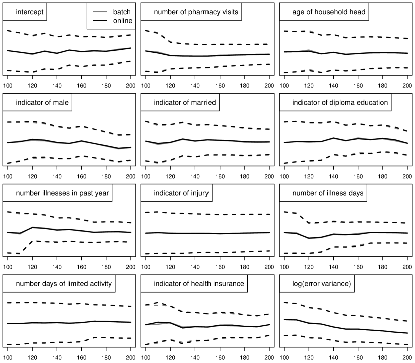
Figure 3: Convergence diagnostics for the example given in Figure 2. The solid lines track the posterior means, whilst the dashed lines show corresponding 95% credible sets. The horizontal axes show the sample sizes between a warm-up batch sample of size $n_{\mbox{\scriptsize warm}}=100$ and validation sample sizes up to $n_{\mbox{\scriptsize valid}}=100$ greater than $n_{\mbox{\scriptsize warm}}$.

Ideally, the online Algorithm 2 will mimic the results of the batch Algorithm 1 as the sample size $n$ increases. However, we know of no guarantees that this will happen and it is possible that the online parameters will diverge from their batch counterparts. For the more elaborate models studied later in this article, such divergence is very common. Therefore, convergence diagnosis at the start of the online iterations is essential. The principal idea is to start by running a small subset of initial data points in the batch algorithm to obtain starting values for both data sufficient statistics and, more importantly, estimated parameters of the model. A second, small validation subset of data is used to compare the batch and online algorithm results. If convergence of the online iterations to their batch counterparts is not verified by this comparison then larger initial batch runs are required to tune the online algorithm.

The idea of collecting streaming data into a small subset before processing it in order to improve performance of a single-pass algorithm is reminiscent of the “mini-batches” of Hoffman, Blei & Bach (2010). However, in our approach, the batching of data happens only with a small subset at the very beginning of the algorithm rather than throughout. Also, we develop an alternative tuning method for this subset batch size below; notably, our tuning method requires batching only some initial subset of the data rather than the full data set.

We will now provide details via the Figure 2 example. Figure 3 shows the posterior means and 95% credible sets for each $\beta_{j}$, $0\leq j\leq 11$, and $\log(\sigma^{2})$ and sample sizes $n=100,110,\ldots,200$ when the Vietnam medical expenses data are fitted via both batch and online MFVB. The batch MFVB summary statistics (shown as grey lines in Figure 3) correspond to simply inputting the first $n_{\mbox{\scriptsize warm}}=100$ observations into Algorithm 1 and then repeating this process for 10 additional equally-spaced sample sizes that are $n_{\mbox{\scriptsize valid}}=100$ greater than $n_{\mbox{\scriptsize warm}}$. The largest sample size is then $n_{\mbox{\scriptsize warm}}+n_{\mbox{\scriptsize valid}}=200$. The online results (shown as grey lines in Figure 3) were obtained via online MFVB updating steps of Algorithm 2 but with $\mu_{q(1/\sigma^{2})}$, $\boldsymbol{y}^{T}\boldsymbol{y}$, $\boldsymbol{X}^{T}\boldsymbol{y}$, $\boldsymbol{X}^{T}\boldsymbol{X}$ and $n$ initialized at the values obtained when the first $n_{\mbox{\scriptsize warm}}=100$ observations are inputted into Algorithm 1. This implies that all the results are identical at $n=n_{\mbox{\scriptsize warm}}=100$, but there are some small discrepancies for $n>100$. In this example the discrepancies are negligible, and hard to discern from Figure 3 – indicating convergence of the online MFVB algorithm. Figure 5 in Section 3 shows an example where convergence is not achieved with $n_{\mbox{\scriptsize warm}}=100$ and a larger warm-up is required.

Algorithm 2’ is a modification of Algorithm 2 that incorporates batch-based tuning and convergence diagnostics. Whilst such modification is not necessary for the example depicted in Figures 2 and 3, it is crucial for more sophisticated semiparametric models such as those described later in this article.

 

• Set $n_{\mbox{\scriptsize warm}}$ to be the warm-up sample size and $n_{\mbox{\scriptsize valid}}$ to be size of the validation period. Read in the first $n_{\mbox{\scriptsize warm}}+n_{\mbox{\scriptsize valid}}$ response and predictor values.

• Create $\boldsymbol{y}_{\mbox{\scriptsize warm}}$ and $\boldsymbol{X}_{\mbox{\scriptsize warm}}$ consisting of the first $n_{\mbox{\scriptsize warm}}$ response and predictor values.

• Feed $\boldsymbol{y}_{\mbox{\scriptsize warm}}$ and $\boldsymbol{X}_{\mbox{\scriptsize warm}}$ into the batch MFVB Algorithm 1 to obtain a starting value for $\mu_{q(1/\sigma^{2})}$.

• Set $\boldsymbol{y}^{T}\boldsymbol{y}\leftarrow\boldsymbol{y}_{\mbox{\scriptsize warm}}^{T}\boldsymbol{y}_{\mbox{\scriptsize warm}}$,  $\boldsymbol{X}^{T}\,\boldsymbol{y}\leftarrow\boldsymbol{X}_{\mbox{\scriptsize warm}}^{T}\boldsymbol{y}_{\mbox{\scriptsize warm}}$,  $\boldsymbol{X}^{T}\boldsymbol{X}\leftarrow\boldsymbol{X}_{\mbox{\scriptsize warm}}^{T}\boldsymbol{X}_{\mbox{\scriptsize warm}}$
  and $n\leftarrow n_{\mbox{\scriptsize warm}}$.

• Run the online MFVB Algorithm 2 until $n=n_{\mbox{\scriptsize warm}}+n_{\mbox{\scriptsize valid}}$.

• Use convergence diagnostic graphics to assess whether the online parameters are converging to the batch parameters.

  • If not converging then return to Step 1 and increase $n_{\mbox{\scriptsize warm}}$.

  • If converging then continue running the online MFVB Algorithm 2 until data no longer available or analysis terminated.

 

Algorithm 2’: Modification of Algorithm 2 to include batch-based tuning and convergence diagnosis.

One could contemplate automating Step 6 of Algorithm 2’, to save the user from having to conduct diagnostic checks. However, we have not yet explored automatic convergence diagnosis and, instead, flag this as a problem worthy of future research.

2.1.2 Model Assumptions

The online MFVB Algorithm 2’ is founded upon the same assumptions as its batch counterpart Algorithm 1. Both algorithms fit the Bayesian linear regression model (1), but the latter has the option to do the fitting in real time for sequentially arriving data.

Throughout this article, we are not allowing for the model parameters to change as new data arrive. Colloquially, we assume “fixed targets” rather than “moving targets”. Extensions to semiparametric regression scenarios where the model parameters drift over time, and real-time algorithms that adapt to such drifts, are certainly worthy of future investigation – but beyond this article’s scope.

2.2 Linear Mixed Models

A very useful structure for semiparametric regression is the class of Bayesian linear mixed models of the form

$$\begin{array}[]{c}\boldsymbol{y}|\,\boldsymbol{\beta},\boldsymbol{u},\sigma_{\varepsilon}^{2}\sim N(\boldsymbol{X}\boldsymbol{\beta}+\boldsymbol{Z}\boldsymbol{u},\sigma_{\varepsilon}^{2}\,\boldsymbol{I})\\[12.91663pt] \boldsymbol{u}|\,\sigma_{u1}^{2},\ldots,\sigma_{ur}^{2}\sim N(\boldsymbol{0},\mbox{blockdiag}(\sigma_{u1}^{2}\,\boldsymbol{I}_{K_{1}},\ldots,\sigma_{ur}^{2}\,\boldsymbol{I}_{K_{r}}))\end{array}$$ (6)

where $\boldsymbol{y}$ is an $n\times 1$ vector of response variables, $\boldsymbol{\beta}$ is a $p\times 1$ vector of fixed effects, $\boldsymbol{u}$ is a vector of random effects, $\boldsymbol{X}$ and $\boldsymbol{Z}$ corresponding design matrices, $\sigma_{\varepsilon}^{2}$ is the error variance and $\sigma_{u1}^{2},\ldots,\sigma_{ur}^{2}$ are variance parameters corresponding to sub-blocks of $\boldsymbol{u}$ of size $K_{1},\ldots,K_{r}$. Here the priors are taken to be

$$\boldsymbol{\beta}\sim N(\boldsymbol{0},\sigma_{\beta}^{2}\boldsymbol{I}),\quad\sigma_{u\ell}\sim\mbox{Half-Cauchy}(A_{u\ell}),\ 1\leq\ell\leq r,\quad\sigma_{\varepsilon}\sim\mbox{Half-Cauchy}(A_{\varepsilon})$$ (7)

with the hyperparameters satisfying $\sigma_{\beta}^{2},A_{\varepsilon},A_{u\ell}>0$ for $1\leq\ell\leq r$. As in Section 2, tractability considerations motivate the introduction of auxiliary variables

$$a_{u\ell}\sim\mbox{Inverse-Gamma}({\textstyle{\frac{1}{2}}},1/A_{u\ell}^{2})\quad\mbox{and}\quad a_{\varepsilon}\sim\mbox{Inverse-Gamma}({\textstyle{\frac{1}{2}}},1/A_{\varepsilon}^{2})$$ (8)

and use of the analogue of (2) to induce Half-Cauchy priors on the standard deviation parameters.

As spelt out in Section 2 of Zhao, Staudenmayer, Coull & Wand (2006), model (6)–(7) encompasses a rich class of models including (with example number from Zhao et al. 2006 added):

• simple random effects models (Examples 1 and 2),

• cross random effects models (Example 3),

• nested random effects models (Example 4),

• generalized additive models (Example 6),

• semiparametric mixed models (Example 7),

• bivariate smoothing and geoadditive models extensions (Example 8).

Examples 2 and 6 of Zhao et al. (2006) actually involve $2\times 2$ and $3\times 3$ unstructured covariance matrix parameters which are not covered by (7). However, as discussed in Section 2.3, the unstructured covariance matrix extension is quite straightforward.

We seek a mean field approximation to the joint posterior density function:

$$p(\boldsymbol{\beta},\boldsymbol{u},a_{u1},\ldots,a_{ur},a_{\varepsilon},\sigma_{u1}^{2},\ldots,\sigma_{ur}^{2},\sigma_{\varepsilon}^{2}|\boldsymbol{y})\approx q(\boldsymbol{\beta},\boldsymbol{u},a_{u1},\ldots,a_{ur},a_{\varepsilon},\sigma_{u1}^{2},\ldots,\sigma_{ur}^{2},\sigma_{\varepsilon}^{2}).$$

The product form

$$q(\boldsymbol{\beta},\boldsymbol{u},a_{u1},\ldots,a_{ur},a_{\varepsilon},\sigma_{u1}^{2},\ldots,\sigma_{ur}^{2},\sigma_{\varepsilon}^{2})=q(\boldsymbol{\beta},\boldsymbol{u},a_{u1},\ldots,a_{ur},a_{\varepsilon})\,q(\sigma_{u1}^{2},\ldots,\sigma_{ur}^{2},\sigma_{\varepsilon}^{2}).$$ (9)

has the advantage of being minimally restrictive whilst also yielding closed form MFVB updates. The analogue of (4) leads to

$$\begin{array}[]{l}q^{*}(\boldsymbol{\beta},\boldsymbol{u},a_{u1},\ldots,a_{ur},a_{\varepsilon})\ \mbox{is the product of the}\ N(\boldsymbol{\mu}_{q(\boldsymbol{\beta},\boldsymbol{u})},\boldsymbol{\Sigma}_{q(\boldsymbol{\beta},\boldsymbol{u})})\ \mbox{density function,}\\[3.22916pt] \mbox{Inverse-Gamma}(1,B_{q(a_{u\ell})})\ \mbox{density functions, $1\leq\ell\leq r$,\ and the}\\[3.22916pt] \mbox{Inverse-Gamma}(1,B_{q(a_{\varepsilon})})\mbox{\ density function;}\\[4.30554pt] q(\sigma_{u1}^{2},\ldots,\sigma_{ur}^{2},\sigma_{\varepsilon}^{2})\ \mbox{is the product of}\mbox{\ Inverse-Gamma}({\textstyle{\frac{1}{2}}}(K_{\ell}+1),B_{q(\sigma^{2}_{u\ell})})\mbox{\ density functions}\\[3.22916pt] \mbox{for $1\leq\ell\leq r$ and the Inverse-Gamma}({\textstyle{\frac{1}{2}}}(n+1),B_{q(\sigma_{\varepsilon}^{2})})\ \mbox{density function.}\end{array}$$

The subscripted $B$s are rate parameters. Batch MFVB fitting of (6), but with slightly different prior distributions, is given by Algorithm 3 of Ormerod & Wand (2010), where the notation

$$\boldsymbol{C}=[\boldsymbol{X}\ \boldsymbol{Z}]$$

is used. Let $P$ be the number of columns in $\boldsymbol{C}$. Then each pass of the corresponding online MFVB algorithm involves arrival and processing of a new scalar response measurement, $y_{\mbox{\tiny new}}$, and a $P\times 1$ vector $\boldsymbol{c}_{\mbox{\tiny new}}$, corresponding to the new row of $\boldsymbol{C}$. This results in Algorithm 3 for real-time fitting of (6).

 

• Perform batch-based tuning runs analogous to those described in Algorithm 2’ and determine a warm-up sample size $n_{\mbox{\scriptsize warm}}$ for which convergence is validated.

• Set $\boldsymbol{y}_{\mbox{\scriptsize warm}}$ and $\boldsymbol{C}_{\mbox{\scriptsize warm}}$ to be the response vector and design matrix based on the first $n_{\mbox{\scriptsize warm}}$ observations. Then set  $\boldsymbol{y}^{T}\boldsymbol{y}\leftarrow\boldsymbol{y}_{\mbox{\scriptsize warm}}^{T}\boldsymbol{y}_{\mbox{\scriptsize warm}}$,  $\boldsymbol{C}^{T}\,\boldsymbol{y}\leftarrow\boldsymbol{C}_{\mbox{\scriptsize warm}}^{T}\boldsymbol{y}_{\mbox{\scriptsize warm}}$,  $\boldsymbol{C}^{T}\boldsymbol{C}\leftarrow\boldsymbol{C}_{\mbox{\scriptsize warm}}^{T}\boldsymbol{C}_{\mbox{\scriptsize warm}}$,  $n\leftarrow n_{\mbox{\scriptsize warm}}$. Also, set $\mu_{q(1/\sigma_{\varepsilon}^{2})}$ and $\mu_{q(1/\sigma_{u1}^{2})},\ldots,\mu_{q(1/\sigma_{ur}^{2})}$ to be the values for these quantities obtained in the batch-based tuning run with sample size $n_{\mbox{\scriptsize warm}}$.

• Cycle:

  • read in $y_{\mbox{\tiny new}}\ (1\times 1)$ and $\boldsymbol{c}_{\mbox{\tiny new}}\ (P\times 1)$   ;  $n\leftarrow n+1$

  • $\boldsymbol{y}^{T}\boldsymbol{y}\leftarrow\boldsymbol{y}^{T}\boldsymbol{y}+y_{\mbox{\tiny new}}^{2}$  ;  $\boldsymbol{C}^{T}\boldsymbol{y}\leftarrow\boldsymbol{C}^{T}\boldsymbol{y}+\boldsymbol{c}_{\mbox{\tiny new}}\,y_{\mbox{\tiny new}}$  ;  $\boldsymbol{C}^{T}\boldsymbol{C}\leftarrow\boldsymbol{C}^{T}\boldsymbol{C}+\boldsymbol{c}_{\mbox{\tiny new}}\,\boldsymbol{c}_{\mbox{\tiny new}}^{T}$

  • $\boldsymbol{\Sigma}_{q(\boldsymbol{\beta},\boldsymbol{u})}\leftarrow\left[\mu_{q(1/\sigma_{\varepsilon}^{2})}\,\boldsymbol{C}^{T}\boldsymbol{C}+\mbox{blockdiag}\{\sigma_{\beta}^{-2}\,\boldsymbol{I}_{p},\mu_{q(1/\sigma_{u1}^{2})}\boldsymbol{I}_{K_{1}},\ldots,\mu_{q(1/\sigma_{ur}^{2})}\boldsymbol{I}_{K_{r}}\}\right]^{-1}$

  • $\boldsymbol{\mu}_{q(\boldsymbol{\beta},\boldsymbol{u})}\leftarrow\mu_{q(1/\sigma_{\varepsilon}^{2})}\,\boldsymbol{\Sigma}_{q(\boldsymbol{\beta},\boldsymbol{u})}\,\boldsymbol{C}^{T}\boldsymbol{y}$   ;   $\mu_{q(1/a_{\varepsilon})}\leftarrow 1/\{\mu_{q(1/\sigma_{\varepsilon}^{2})}+A_{\varepsilon}^{-2}\}$

  • $\mu_{q(1/\sigma_{\varepsilon}^{2})}\leftarrow\displaystyle{\frac{n+1}{2\,\mu_{q(1/a_{\varepsilon})}+\boldsymbol{y}^{T}\boldsymbol{y}-2\boldsymbol{\mu}_{q(\boldsymbol{\beta},\boldsymbol{u})}^{T}\boldsymbol{C}^{T}\boldsymbol{y}+\mbox{tr}[(\boldsymbol{C}^{T}\boldsymbol{C})\{\boldsymbol{\Sigma}_{q(\boldsymbol{\beta},\boldsymbol{u})}+\boldsymbol{\mu}_{q(\boldsymbol{\beta},\boldsymbol{u})}\boldsymbol{\mu}_{q(\boldsymbol{\beta},\boldsymbol{u})}^{T}\}]}}$

  • For $\ell=1,\ldots,r$ :

    • $\mu_{q(1/a_{u\ell})}\leftarrow 1/\{\mu_{q(1/\sigma_{u\ell}^{2})}+A_{u\ell}^{-2}\}$

    • $\mu_{q(1/\sigma_{u\ell}^{2})}\leftarrow\displaystyle{\frac{K_{\ell}+1}{2\,\mu_{q(1/a_{u\ell})}+\|\boldsymbol{\mu}_{q(\boldsymbol{u}_{\ell})}\|^{2}+\mbox{tr}(\boldsymbol{\Sigma}_{q(\boldsymbol{u}_{\ell})})}}$

• until data no longer available or analysis terminated.

 

Algorithm 3 Online mean field variational Bayes algorithm for approximate inference in the Gaussian response linear mixed model (6).

The $\boldsymbol{c}_{\mbox{\tiny new}}$ vector will have different forms depending on the type of linear mixed model. To better understand the nature of these forms, consider the following two special cases of (6):

$$\begin{array}[]{c}y_{ij}|\beta_{0},U_{i},\beta_{1},\sigma_{\varepsilon}^{2}\stackrel{{\scriptstyle{\tiny\mbox{ind.}}}}{{\sim}}N(\beta_{0}+U_{i}+\beta_{1}\,x_{ij},\sigma_{\varepsilon}^{2}),\quad 1\leq i\leq m,\quad 1\leq j\leq n_{i},\\[4.30554pt] U_{i}|\,\sigma_{u}^{2}\stackrel{{\scriptstyle{\tiny\mbox{ind.}}}}{{\sim}}N(0,\sigma_{u}^{2}\,\boldsymbol{I}),\quad\beta_{0},\beta_{1}\stackrel{{\scriptstyle{\tiny\mbox{ind.}}}}{{\sim}}N(0,\sigma_{\boldsymbol{\beta}}^{2}),\\[4.30554pt] \sigma_{u}\sim\mbox{Half-Cauchy}(A_{u}),\quad\sigma_{\varepsilon}\sim\mbox{Half-Cauchy}(A_{\varepsilon})\end{array}$$ (10)

and

$$\begin{array}[]{c}y_{i}|\beta_{0},\beta_{s},\beta_{t},\boldsymbol{u}_{s},\boldsymbol{u}_{t},\sigma_{\varepsilon}^{2}\stackrel{{\scriptstyle{\tiny\mbox{ind.}}}}{{\sim}}N\left(\beta_{0}+\beta_{s}\,s_{i}+\beta_{t}\,t_{i}+{\displaystyle\sum_{k=1}^{K_{s}}}\,u_{s,k}\,z_{k}^{s}(s_{i})+{\displaystyle\sum_{k=1}^{K_{t}}}\,u_{t,k}\,z_{k}^{t}(t_{i}),\sigma_{\varepsilon}^{2}\right),\\[4.30554pt] \quad 1\leq i\leq n,\quad\boldsymbol{u}_{s}=[u_{s,1},\ldots,u_{s,K_{s}}]^{T},\quad\boldsymbol{u}_{t}=[u_{t,1},\ldots,u_{t,K_{t}}]^{T},\\[4.30554pt] \boldsymbol{u}_{s}|\,\sigma_{u,s}^{2}\sim N(0,\sigma_{u,s}^{2}\,\boldsymbol{I}),\quad\boldsymbol{u}_{t}|\,\sigma_{u,t}^{2}\sim N(0,\sigma_{u,t}^{2}\,\boldsymbol{I}),\\[4.30554pt] \beta_{0},\beta_{s},\beta_{t}\stackrel{{\scriptstyle{\tiny\mbox{ind.}}}}{{\sim}}N(0,\sigma_{\boldsymbol{\beta}}^{2}),\quad\sigma_{u,s}\sim\mbox{Half-Cauchy}(A_{u,s}),\quad\sigma_{u,t}\sim\mbox{Half-Cauchy}(A_{u,t}),\\[4.30554pt] \sigma_{\varepsilon}\sim\mbox{Half-Cauchy}(A_{\varepsilon}).\end{array}$$ (11)

Here and throughout $\stackrel{{\scriptstyle{\tiny\mbox{ind.}}}}{{\sim}}$ denotes “distributed independently”.

Model (10) is the random intercept extension of simple linear regression for longitudinal data with $(x_{ij},y_{ij})$ denoting the $j$th predictor/response pair for the $i$th group, with $m$ denoting the number of groups. There is no intrinsic reason to insist that the observations arrive in order with respect to the $i,j$ subscripting. Hence $\boldsymbol{c}_{\mbox{\tiny new}}$ will have the form

$$\boldsymbol{c}_{\mbox{\tiny new}}=\left[\begin{array}[]{c}1\\ x_{\mbox{{\tiny new}}}\\ \boldsymbol{e}_{\mbox{\tiny new}}\\ \end{array}\right]$$

where $x_{\mbox{{\tiny new}}}$ is the new predictor measurement that partners $y_{\mbox{\tiny new}}$ and $\boldsymbol{e}_{\mbox{\tiny new}}$ is a $m\times 1$ vector with an entry of 1 in position $i_{\mbox{\tiny new}}$, corresponding to the group that $(x_{\mbox{{\tiny new}}},y_{\mbox{\tiny new}})$ is from, and zeroes elsewhere.

Model (11) is a mixed model-based penalized spline version of the additive model

$$y_{i}=\beta_{0}+f_{s}(s_{i})+f_{t}(t_{i})+\varepsilon_{i},\quad 1\leq i\leq n,$$

where the $s_{i}$ and $t_{i}$ are continuous predictor measurements and $f_{s}$ and $f_{t}$ are smooth functions. The functions $z_{k}^{s}(\cdot)$, $1\leq k\leq K_{s}$, are spline basis functions. A simple example is the truncated line basis

$$z_{k}^{s}(s)=(s-\kappa^{s}_{k})_{+}$$ (12)

where $\kappa^{s}_{1},\ldots,\kappa^{s}_{K_{s}}$ are a set of knots within the domain of the $s_{i}$ values. More sophisticated, and numerically stable, options for $z_{k}(s)$ are described in, for example, Wood (2006), Welham et al. (2007) and Wand & Ormerod (2008). We use the last of these, known as O’Sullivan splines, in our examples. The $z_{k}^{t}(\cdot)$, $1\leq k\leq K_{t}$, are defined similarly. A key feature of the $z_{k}^{s}(\cdot)$ and $z_{k}^{t}(\cdot)$ is that the multiple-of-diagonal covariance matrices are appropriate under mixed model representations of penalized splines. This subtlety is explained in Section 4 of Wand & Ormerod (2008).

Online fitting of (11) involves reading in vectors of the form

$$\boldsymbol{c}_{\mbox{\tiny new}}=[1,s_{\mbox{\tiny new}},t_{\mbox{\tiny new}},z_{1}^{s}(s_{\mbox{\tiny new}}),\ldots,z_{K_{s}}^{s}(s_{\mbox{\tiny new}}),z_{1}^{t}(t_{\mbox{\tiny new}}),\ldots,z_{K_{t}}^{t}(t_{\mbox{\tiny new}})]^{T}$$

where $s_{\mbox{\tiny new}}$ and $t_{\mbox{\tiny new}}$ are the new predictor measurements that partner $y_{\mbox{\tiny new}}$. There is, however, the issue of having to set the spline basis functions in advance. For instance, if the truncated line basis (12) is used then the knots have to be set at or near the start of the algorithm. For many applications this is not a major problem. For example, if the $s_{\mbox{\tiny new}}$ values correspond to age, in years, of human adults then the range of possible $s_{i}$ values is easy to specify and a reasonable spline basis can be set in advance. In a similar vein, for longitudinal data, Algorithm 3 assumes that the number of groups is set in advance. If the groups correspond to the counties of a geographical entity then this should not pose a problem. If the data are from a medical study then Algorithm 3 assumes that the number of patients and their identity numbers are fixed in advance. If this is not a reasonable assumption then some adjustment is required.

Finally, we mention the possibility of speeding up the most expensive update:

$$\boldsymbol{\Sigma}_{q(\boldsymbol{\beta},\boldsymbol{u})}\leftarrow\left[\mu_{q(1/\sigma_{\varepsilon}^{2})}\,\boldsymbol{C}^{T}\boldsymbol{C}+\mbox{blockdiag}\{\sigma_{\beta}^{-2}\,\boldsymbol{I}_{p},\mu_{q(1/\sigma_{u1}^{2})}\boldsymbol{I}_{K_{1}},\ldots,\mu_{q(1/\sigma_{ur}^{2})}\boldsymbol{I}_{K_{r}}\}\right]^{-1}.$$ (13)

For Model (10) the matrix requiring inversion has dimension $(2+m)\times(2+m)$. If the number of groups is high then naïve implementation could lead to a bottleneck at (13). In the batch case it is well-known (e.g. Smith & Wand, 2008) that $\boldsymbol{C}^{T}\boldsymbol{C}$ contains diagonal forms that allow $O(m)$ computation of the right-hand side of (13). Such efficiencies are available in the online case, but require careful rearrangement of the entries of $\boldsymbol{C}^{T}\boldsymbol{C}$ during the updates.

2.3 Extension to Unstructured Covariance Matrices for Random Effects

A random intercepts and slopes extension of (10) is one with the first two hierarchical levels set to

$$\begin{array}[]{c}y_{ij}|\beta_{0},\beta_{1},U_{i},V_{i},\sigma_{\varepsilon}^{2}\stackrel{{\scriptstyle{\tiny\mbox{ind.}}}}{{\sim}}N(\beta_{0}+U_{i}+(\beta_{1}+V_{i})\,x_{ij},\sigma_{\varepsilon}^{2}),\quad 1\leq i\leq m,\quad 1\leq j\leq n_{i},\\[8.61108pt] \mbox{and}\quad\left[\begin{array}[]{c}U_{i}\\ V_{i}\\ \end{array}\right]\Big{|}\boldsymbol{\Sigma}\sim N(\boldsymbol{0},\boldsymbol{\Sigma}),\quad\mbox{where}\quad\boldsymbol{\Sigma}\equiv\left[\begin{array}[]{cc}\sigma_{u}^{2}&\rho_{uv}\,\sigma_{u}\,\sigma_{v}\\ \rho_{uv}\,\sigma_{u}\,\sigma_{v}&\sigma_{v}^{2}\end{array}\right]\end{array}$$

is an unstructured $2\times 2$ covariance matrix. The conjugate prior for $\boldsymbol{\Sigma}$ is the Inverse Wishart distribution. However, the specification

$$\begin{array}[]{c}\boldsymbol{\Sigma}|\,a_{uv1},a_{uv2}\sim\mbox{Inverse-Wishart}\left(\nu+1,2\nu\,\left[\begin{array}[]{cc}1/a_{uv1}&0\\ 0&1/a_{uv2}\end{array}\right]\right),\\[8.61108pt] a_{uv1},a_{uv2}\stackrel{{\scriptstyle{\tiny\mbox{ind.}}}}{{\sim}}\mbox{Inverse-Gamma}({\textstyle{\frac{1}{2}}},1/A_{uv}),\quad\nu,A_{uv}>0\end{array}$$

provides a covariance matrix extension of $\sigma_{u}\sim\mbox{Half-Cauchy}(A_{u})$. The choice $\nu=2$ is particularly attractive since it imposes a $\mbox{Uniform}(-1,1)$ distribution on $\rho_{uv}$ and Half-$t_{2}$ distributions on $\sigma_{u}$ and $\sigma_{v}$. This is laid out in Huang & Wand (2012), including the definition of the $\mbox{Inverse-Wishart}(a,\boldsymbol{B})$ distribution.

Extensions to more sophisticated models, possibly having larger unstructured covariance matrices, can be done in a similar fashion.

2.4 Extension to Sparse Shrinkage Penalties

Model (6) involves the following Gaussian penalization on sub-vectors of $\boldsymbol{u}$:

$$\boldsymbol{u}_{\ell}|\,\sigma_{u\ell}^{2}\sim N(\boldsymbol{0},\sigma_{u\ell}^{2}\,\boldsymbol{I}),\quad 1\leq\ell\leq r.$$ (14)

However, many models of current-day interest, such as wide data (“$p\gg n$”) and wavelet regression, require an assumption that the regression coefficients are sparse. Under such sparseness assumptions, the Gaussian priors (14) are not appropriate since they induce a relatively gentle amount of penalization that lacks the ability to annihilate regression coefficients during fitting and inference.

For simplicity of exposition we will confine discussion of the sparse shrinkage extension to the $r=1$ version of (6). Hence we retain

$$y\,|\,\boldsymbol{\beta},\boldsymbol{u},\sigma_{\varepsilon}^{2}\sim N(\boldsymbol{X}\boldsymbol{\beta}+\boldsymbol{Z}\,\boldsymbol{u},\sigma_{\varepsilon}^{2}\boldsymbol{I})$$

without any sub-division of $\boldsymbol{u}$. Let $K$ be the dimension of $\boldsymbol{u}$ and consider general mutually independent prior penalizations of the form:

$$u_{k}\stackrel{{\scriptstyle{\tiny\mbox{ind.}}}}{{\sim}}p(u;\sigma_{u},\boldsymbol{\theta})$$

where $p(\cdot;\sigma_{u},\boldsymbol{\theta})$ is a density function with scale parameter $\sigma_{u}$ and shape parameter $\boldsymbol{\theta}$. Options for $p(u;1,\boldsymbol{\theta})$ include:

$${\begin{array}[]{rcll}p(u;1,w)&=&w\{{\textstyle{\frac{1}{2}}}\exp(-|u|)\}+(1-w)\,\delta_{0}(u)&\ \mbox{(Laplace-Zero),}\\[8.61108pt] p(u;1)&=&(2\pi^{3})^{-1/2}\exp(u^{2}/2)E_{1}(u^{2}/2)&\ \mbox{(Horseshoe),}\\[8.61108pt] p(u;1,\lambda)&=&\frac{\lambda\,2^{\lambda}\Gamma(\lambda+{\textstyle{\frac{1}{2}}})}{\pi^{1/2}}\,\exp(u^{2}/4)\,D_{-2\lambda-1}(|u|)&\ \mbox{(Normal-Exponential-Gamma)}\\[8.61108pt] \mbox{and}\quad p(u;\lambda)&=&\displaystyle{\frac{1}{2(1+|u|/\lambda)^{\lambda+1}}}&\ \mbox{(Generalized Double Pareto).}\\ \end{array}}$$ (15)

Here $\delta_{0}$ denotes the Dirac delta function with mass at zero. Also, $E_{1}$ denotes the exponential integral function of order 1 and $D_{\nu}$ denotes the parabolic cylinder function of order $\nu$ according to the definitions of Gradshteyn & Ryzhik (1994). References for the development of these sparse shrinkage priors are Johnstone & Silverman (2005) (Laplace-Zero), Carvalho, Polson & Scott (2010) (Horseshoe), Griffin & Brown (2011) (Normal-Exponential-Gamma) and Armagan, Dunson & Lee (2012) (Generalized Double Pareto).

Batch MFVB algorithms for the priors (15) recently have been derived by Wand & Ormerod (2011) (Laplace-Zero prior) and Neville, Ormerod & Wand (2012) (Horseshoe, Normal-Exponential-Gamma and Generalized Double Pareto priors).

Algorithm 4 is the online adaptation of Algorithm 4 of Wand & Ormerod (2011) for the Laplace-Zero prior model:

$$\begin{array}[]{c}\boldsymbol{y}|\boldsymbol{\beta},\boldsymbol{\gamma},\boldsymbol{v},\sigma_{\varepsilon}^{2}\sim N(\boldsymbol{X}\boldsymbol{\beta}+\boldsymbol{Z}(\boldsymbol{\gamma}\odot\boldsymbol{v}),\sigma_{\varepsilon}^{2}\boldsymbol{I}),\quad\boldsymbol{v}|\,\sigma_{u}^{2},\boldsymbol{b}\sim N(\boldsymbol{0},\sigma_{u}^{2}\,\mbox{diag}(\boldsymbol{b})^{-1}),\\ \hbox{}\hfil\\ \sigma^{2}_{u}|\,a_{u}\sim\mbox{Inverse-Gamma}({\textstyle{\frac{1}{2}}},1/a_{u}),\quad\sigma_{\varepsilon}^{2}|\,a_{\varepsilon}\sim\mbox{Inverse-Gamma}({\textstyle{\frac{1}{2}}},1/a_{\varepsilon}),\\ \hbox{}\hfil\\ \boldsymbol{\beta}\sim N(\boldsymbol{0},\sigma_{\beta}^{2}\boldsymbol{I}),\ a_{u}\sim\mbox{Inverse-Gamma}({\textstyle{\frac{1}{2}}},1/A_{u}^{2}),\ a_{\varepsilon}\sim\mbox{Inverse-Gamma}({\textstyle{\frac{1}{2}}},1/A_{\varepsilon}^{2}),\\ \hbox{}\hfil\\ b_{k}\stackrel{{\scriptstyle{\tiny\mbox{ind.}}}}{{\sim}}\mbox{Inverse-Gamma}(1,{\textstyle{\frac{1}{2}}}),\quad\gamma_{k}|\,\rho\sim\mbox{Bernoulli}(\rho),\quad\rho\stackrel{{\scriptstyle{\tiny\mbox{ind.}}}}{{\sim}}\mbox{Beta}(A_{\rho},B_{\rho}).\end{array}$$ (16)

Note that $\boldsymbol{A}\odot\boldsymbol{B}$ denotes the element-wise product of matrices $\boldsymbol{A}$ and $\boldsymbol{B}$ having the same dimensions. Model (16) is a reproduction of (30) in Wand & Ormerod (2011) and the additional notation is explained there. Note, in particular, that the Laplace-Zero prior is handled via the introduction of auxiliary variables $\boldsymbol{b}$, $\boldsymbol{\gamma}$ and $\boldsymbol{v}$. Section 3.6 of Wand & Ormerod (2011) provides the necessary details. Similar online MFVB algorithms for the continuous sparse signal shrinkage priors listed in (15) follow from the batch MFVB algorithms of Neville, Ormerod & Wand (2012).

 

• Perform batch-based tuning runs analogous to those described in Algorithm 2’ and determine a warm-up sample size $n_{\mbox{\scriptsize warm}}$ for which convergence is validated. The batch MFVB algorithm is Algorithm 4 of Wand & Ormerod (2011).

• Set $\boldsymbol{y}_{\mbox{\scriptsize warm}}$ and $\boldsymbol{C}_{\mbox{\scriptsize warm}}=[\boldsymbol{1}\ \boldsymbol{Z}_{\mbox{\scriptsize warm}}]$ to be the response vector and design matrix based on the first $n_{\mbox{\scriptsize warm}}$ observations. Then set  $\boldsymbol{y}^{T}\boldsymbol{y}\leftarrow\boldsymbol{y}_{\mbox{\scriptsize warm}}^{T}\boldsymbol{y}_{\mbox{\scriptsize warm}}$,  $\boldsymbol{Z}^{T}\boldsymbol{1}\leftarrow\boldsymbol{Z}_{\mbox{\scriptsize warm}}^{T}\boldsymbol{1}$,  $\boldsymbol{Z}^{T}\boldsymbol{y}\leftarrow\boldsymbol{Z}_{\mbox{\scriptsize warm}}^{T}\boldsymbol{y}$,  $\boldsymbol{Z}^{T}\boldsymbol{Z}\leftarrow\boldsymbol{Z}_{\mbox{\scriptsize warm}}^{T}\boldsymbol{Z}_{\mbox{\scriptsize warm}}$,  $\boldsymbol{C}^{T}\,\boldsymbol{y}\leftarrow\boldsymbol{C}_{\mbox{\scriptsize warm}}^{T}\boldsymbol{y}_{\mbox{\scriptsize warm}}$,  $\boldsymbol{C}^{T}\boldsymbol{C}\leftarrow\boldsymbol{C}_{\mbox{\scriptsize warm}}^{T}\boldsymbol{C}_{\mbox{\scriptsize warm}}$,  $n\leftarrow n_{\mbox{\scriptsize warm}}$. Set $K$ to be the number of columns in $\boldsymbol{Z}_{\mbox{\scriptsize warm}}$. Also, set $\mu_{q(1/\sigma^{2}_{\varepsilon})},\ \mu_{q(1/\sigma^{2}_{u})},\ \mu_{q(1/a_{\varepsilon})},\ \mu_{q(1/a_{u})},\boldsymbol{\mu}_{q(\boldsymbol{b})},\boldsymbol{\mu}_{q(\boldsymbol{w}_{\boldsymbol{\gamma}})}\ \mbox{and}\ \boldsymbol{\Omega}_{q(\boldsymbol{w}_{\boldsymbol{\gamma}})}$ to be the values for these quantities obtained in the batch-based tuning run with sample size $n_{\mbox{\scriptsize warm}}$.

• Cycle:

  • read in $y_{\mbox{\tiny new}}\ (1\times 1)$ and $\boldsymbol{z}_{\mbox{\tiny new}}\ (K\times 1)$   ;  $n\leftarrow n+1$  ;  $\boldsymbol{c}_{\mbox{\tiny new}}\leftarrow\left[\begin{array}[]{c}1\\ \boldsymbol{z}_{\mbox{\tiny new}}\end{array}\right]$

  • $\boldsymbol{y}^{T}\boldsymbol{y}\leftarrow\boldsymbol{y}^{T}\boldsymbol{y}+y_{\mbox{\tiny new}}^{2}$  ;  $\boldsymbol{Z}^{T}\boldsymbol{1}\leftarrow\boldsymbol{Z}^{T}\boldsymbol{1}+\boldsymbol{z}_{\mbox{\tiny new}}$  ;  $\boldsymbol{Z}^{T}\boldsymbol{y}\leftarrow\boldsymbol{Z}^{T}\boldsymbol{y}+\boldsymbol{z}_{\mbox{\tiny new}}\,y_{\mbox{\tiny new}}$

  • $\boldsymbol{Z}^{T}\boldsymbol{Z}\leftarrow\boldsymbol{Z}^{T}\boldsymbol{Z}+\boldsymbol{z}_{\mbox{\tiny new}}\,\boldsymbol{z}_{\mbox{\tiny new}}^{T}$  ;  $\boldsymbol{C}^{T}\boldsymbol{y}\leftarrow\boldsymbol{C}^{T}\boldsymbol{y}+\boldsymbol{c}_{\mbox{\tiny new}}\,y_{\mbox{\tiny new}}$  ;  $\boldsymbol{C}^{T}\boldsymbol{C}\leftarrow\boldsymbol{C}^{T}\boldsymbol{C}+\boldsymbol{c}_{\mbox{\tiny new}}\,\boldsymbol{c}_{\mbox{\tiny new}}^{T}$

  • $\boldsymbol{\Sigma}_{q(\boldsymbol{\beta},\boldsymbol{v})}\leftarrow\Bigg{(}\mu_{q(1/\sigma_{\varepsilon}^{2})}(\boldsymbol{C}^{T}\boldsymbol{C})\odot\boldsymbol{\Omega}_{q(\boldsymbol{w}_{\boldsymbol{\gamma}})}+\left[\begin{array}[]{cc}\sigma_{\beta}^{-2}&\boldsymbol{0}\\ \boldsymbol{0}&\mu_{q(1/\sigma_{u}^{2})}\mbox{diag}(\boldsymbol{\mu}_{q(\boldsymbol{b})})\end{array}\right]\Bigg{)}^{-1}$

  • $\boldsymbol{\mu}_{q(\boldsymbol{\beta},\boldsymbol{v})}\leftarrow\mu_{q(1/\sigma_{\varepsilon}^{2})}\boldsymbol{\Sigma}_{q(\boldsymbol{\beta},\boldsymbol{v})}\mbox{diag}\{\boldsymbol{\mu}_{q(\boldsymbol{w}_{\boldsymbol{\gamma}})}\}\boldsymbol{C}^{T}\boldsymbol{y}$

  • $\mu_{q(\boldsymbol{b})}\leftarrow[\mu_{q(1/\sigma_{u}^{2})}\{\mbox{diagonal}(\Sigma_{q(\boldsymbol{v})})+\boldsymbol{\mu}^{2}_{q(\boldsymbol{v})}\}]^{-1/2}$

  • $$\boldsymbol{\eta}_{q(\boldsymbol{\gamma})} \leftarrow -{\textstyle{\frac{1}{2}}}\,\mu_{q(1/\sigma_{\varepsilon}^{2})}\Big{[}\mbox{diagonal}(\boldsymbol{Z}^{T}\boldsymbol{Z})\odot\{\boldsymbol{\sigma}^{2}_{q(\boldsymbol{v})}+\boldsymbol{\mu}^{2}_{q(\boldsymbol{v})}\}-2(\boldsymbol{Z}^{T}\boldsymbol{y})\odot\boldsymbol{\mu}_{q(\boldsymbol{v})}$$

    $$\quad+2(\boldsymbol{Z}^{T}\boldsymbol{1})\odot\{[\boldsymbol{\Sigma}_{q(\boldsymbol{\beta},\boldsymbol{v})})]_{i=1,2\leq j\leq K+1}+\mu_{q(\beta)}\boldsymbol{\mu}_{q(\boldsymbol{v})}\}$$

    $$\quad+2\,\mbox{diagonal}\{\boldsymbol{Z}^{T}\boldsymbol{Z}\,\mbox{diag}(\boldsymbol{\mu}_{q(\boldsymbol{\gamma})})\boldsymbol{\Sigma}_{q(\boldsymbol{v})}\}$$

    $$\quad-2\,\mbox{diagonal}(\boldsymbol{Z}^{T}\boldsymbol{Z})\odot\boldsymbol{\mu}_{q(\boldsymbol{\gamma})}\odot\mbox{diagonal}(\boldsymbol{\Sigma}_{q(\boldsymbol{v})})$$

    $$\quad+2\boldsymbol{\mu}_{q(\boldsymbol{v})}\odot\{\boldsymbol{Z}^{T}\boldsymbol{Z}(\boldsymbol{\mu}_{q(\boldsymbol{\gamma})}\odot\boldsymbol{\mu}_{q(\boldsymbol{v})})-\mbox{diagonal}(\boldsymbol{Z}^{T}\boldsymbol{Z})\odot\boldsymbol{\mu}_{q(\boldsymbol{\gamma})}\odot\boldsymbol{\mu}_{q(\boldsymbol{v})}\}\Big{]}$$

    $$\quad+\psi(A_{\rho}+\mu_{q(\gamma_{\bullet})})-\psi(B_{\rho}+K-\mu_{q(\gamma_{\bullet})})$$

  • $\mu_{q(\boldsymbol{\gamma})}\leftarrow\displaystyle{\frac{\exp(\eta_{q(\boldsymbol{\gamma})})}{1+\exp(\eta_{q(\boldsymbol{\gamma})})}}$    ;   $\boldsymbol{\mu}_{q(\boldsymbol{w}_{\boldsymbol{\gamma}})}\leftarrow\left[\begin{array}[]{c}1\\ \boldsymbol{\mu}_{q(\boldsymbol{\gamma})}\end{array}\right]$   ;   $\mu_{q(\gamma_{\bullet})}\leftarrow\sum_{k=1}^{K}\mu_{q(\gamma_{k})}$

  • $\boldsymbol{\Omega}_{q(\boldsymbol{w}_{\boldsymbol{\gamma}})}\leftarrow\mbox{diag}\{\boldsymbol{\mu}_{q(\boldsymbol{w}_{\boldsymbol{\gamma}})}\odot(\boldsymbol{1}-\boldsymbol{\mu}_{q(\boldsymbol{w}_{\boldsymbol{\gamma}})})\}+\boldsymbol{\mu}_{q(\boldsymbol{w}_{\boldsymbol{\gamma}})}\,\boldsymbol{\mu}_{q(\boldsymbol{w}_{\boldsymbol{\gamma}})}^{T}$

  • $\mu_{q(1/a_{\varepsilon})}\leftarrow 1/\{\mu_{q(1/\sigma_{\varepsilon}^{2})}+A_{\varepsilon}^{-2}\}$   ;  $\mu_{q(1/a_{u})}\leftarrow 1/\{\mu_{q(1/\sigma_{u}^{2})}+A_{u}^{-2}\}$

  • $\begin{array}[]{l}B_{q(\sigma_{\varepsilon}^{2})}\leftarrow\mu_{q(1/a_{\varepsilon})}+{\textstyle{\frac{1}{2}}}\,\boldsymbol{y}^{T}\boldsymbol{y}-\left(\boldsymbol{\mu}_{q(\boldsymbol{w}_{\boldsymbol{\gamma}})}\odot\mu_{q(\boldsymbol{\beta},\boldsymbol{v})}\right)^{T}\,\boldsymbol{C}^{T}\boldsymbol{y}\\ \qquad\qquad+{\textstyle{\frac{1}{2}}}\mbox{tr}\left(\boldsymbol{C}^{T}\boldsymbol{C}\,\,\left[\boldsymbol{\Omega}_{q(\boldsymbol{w}_{\boldsymbol{\gamma}})}\odot\left\{\boldsymbol{\Sigma}_{q(\boldsymbol{\beta},\boldsymbol{v})}+\boldsymbol{\mu}_{q(\boldsymbol{\beta},\boldsymbol{v})}\boldsymbol{\mu}_{q(\boldsymbol{\beta},\boldsymbol{v})}^{T}\right\}\right]\right)\end{array}$

  • $B_{q(\sigma^{2}_{u})}\leftarrow\mu_{q(1/a_{u})}+{\textstyle{\frac{1}{2}}}\boldsymbol{\mu}_{q(\boldsymbol{b})}^{T}\{\mbox{diagonal}(\boldsymbol{\Sigma}_{q(\boldsymbol{v})})+\boldsymbol{\mu}_{q(\boldsymbol{v})}^{2}\}$

  • $\mu_{q(1/\sigma_{u}^{2})}\leftarrow{\textstyle{\frac{1}{2}}}(K+1)/B_{q(\sigma^{2}_{u})}$   ;  $\mu_{q(1/\sigma_{\varepsilon}^{2})}\leftarrow{\textstyle{\frac{1}{2}}}(n+1)/B_{q(\sigma_{\varepsilon}^{2})}$

  until data no longer available or analysis terminated.

 

Algorithm 4 Mean field variational Bayes algorithm for the determination of the optimal parameters in $q^{*}(\boldsymbol{\beta},\boldsymbol{v})$, $q^{*}(\boldsymbol{\gamma})$, $q^{*}(\sigma^{2}_{u})$ and $q^{*}(\sigma_{\varepsilon}^{2})$ for the Bayesian sparse signal regression model (16).

As with the spline-based semiparametric regression models described in Section 2.2, the wavelet-based models described here benefit from the low-rank property laid out in Section 3.1 of Wand & Ormerod (2011). This property entails that the basis functions are fixed once and for all during the warm-up period. This permits fast updating of wavelet nonparametric fits as new data arrive. A cost of this approach is that the domain of predictors needs to be specified based on the warm-up data. As explained in Section 2.2, this will often be reasonable. Of course, there is always the possibility of new predictor values landing outside domain of the basis functions, in which case some modification may be necessary.

Figure 4 illustrates online wavelet nonparametric regression for data generated to

$$x_{\mbox{{\tiny new}}}\sim\mbox{Uniform(0,1)},\quad y_{\mbox{\tiny new}}|\,x_{\mbox{{\tiny new}}}\sim N(f_{\mbox{\tiny WO}}(x_{\mbox{{\tiny new}}}),1)$$

where $f_{\mbox{\tiny WO}}$ is defined by (20) of Wand & Ormerod (2011). The warm-up sample size is $n_{\mbox{\scriptsize warm}}=300$. The desired improvement in the estimate of $f_{\mbox{\tiny WO}}$ as $n$ increases is clearly apparent. Convergence to the batch MFVB estimate was found to be excellent in this case.

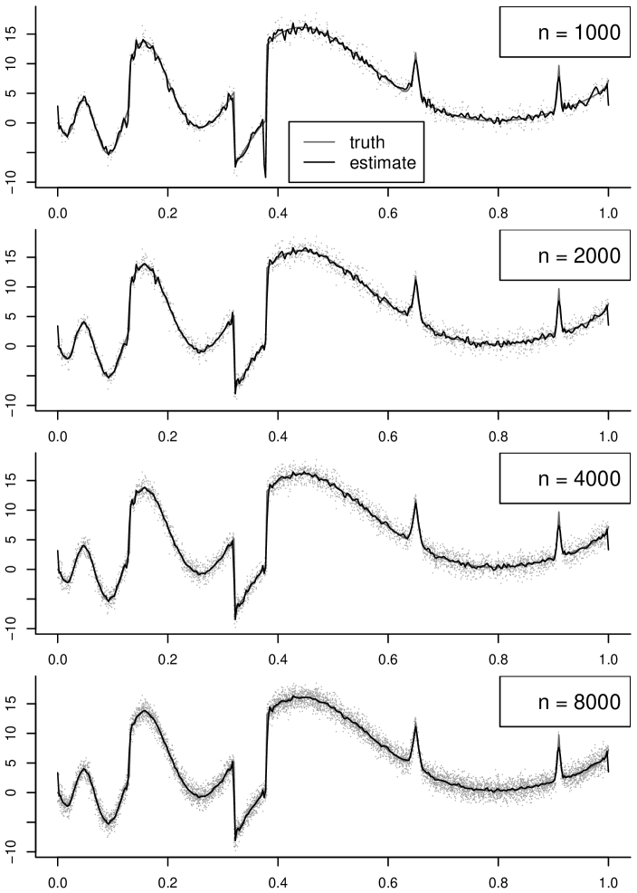
Figure 4: Examples of online MFVB wavelet fits based on Algorithm 4. The true regression curve is the function $f_{\mbox{\tiny WO}}$ defined in Wand & Ormerod (2011).

3 Binary Response Models

The binary response model we consider here takes the same form as (6) and (7), but with $\sigma_{\varepsilon}$ removed and

$$\boldsymbol{y}|\,\boldsymbol{\beta},\boldsymbol{u}\sim\mbox{Bernoulli}\{\mbox{logit}^{-1}(\boldsymbol{X}\,\boldsymbol{\beta}+\boldsymbol{Z}\,\boldsymbol{u})\}.$$ (17)

Note that (17) is a convenient shorthand for the entries of $\boldsymbol{y}$, conditional on $(\boldsymbol{\beta},\boldsymbol{u})$, being independent and with $i$th entry $\mbox{Bernoulli}[\mbox{logit}^{-1}\{(\boldsymbol{X}\,\boldsymbol{\beta}+\boldsymbol{Z}\,\boldsymbol{u})_{i}\}]$.

Batch MFVB algorithms for approximate inference in (17), (6) and (7) start with the product restriction

$$p(\boldsymbol{\beta},\boldsymbol{u},a_{u1},\ldots,a_{ur},\sigma_{u1}^{2},\ldots,\sigma_{ur}^{2})\approx q(\boldsymbol{\beta},\boldsymbol{u},a_{u1},\ldots,a_{ur})\,q(\sigma_{u1}^{2},\ldots,\sigma_{ur}^{2}).$$

The resultant updates for the $\sigma_{u\ell}^{2}$ and $a_{u\ell}$ are the same as in the Gaussian response case. The optimal $q$-density for $(\boldsymbol{\beta},\boldsymbol{u})$ satisfies

$$q^{*}(\boldsymbol{\beta},\boldsymbol{u})\propto\exp\left\{\boldsymbol{y}^{T}(\boldsymbol{X}\boldsymbol{\beta}+\boldsymbol{Z}\boldsymbol{u})-\boldsymbol{1}^{T}\log(1+e^{\boldsymbol{X}\boldsymbol{\beta}+\boldsymbol{Z}\boldsymbol{u}})-\frac{1}{2\sigma^{2}_{\beta}}\|\boldsymbol{\beta}\|^{2}-{\textstyle{\frac{1}{2}}}\sum_{\ell=1}^{L}\mu_{q(1/\sigma_{u\ell}^{2})}\,\|\boldsymbol{u}_{\ell}\|^{2}\right\}.$$ (18)

However, this is a non-standard form and poses tractability problems with regards to approximate inference for $(\boldsymbol{\beta},\boldsymbol{u})$. A reasonable remedy is to replace (18) by a member of the following family of Multivariate Normal approximations:

$$\underline{q}^{*}(\boldsymbol{\beta},\boldsymbol{u})\sim N(\boldsymbol{\mu}_{\underline{q}(\boldsymbol{\beta},\boldsymbol{u};\boldsymbol{\xi})},\boldsymbol{\Sigma}_{\underline{q}(\boldsymbol{\beta},\boldsymbol{u};\boldsymbol{\xi})})$$

where

$$\boldsymbol{\Sigma}_{\underline{q}(\boldsymbol{\beta},\boldsymbol{u})}\equiv\left[2\boldsymbol{C}^{T}\mbox{diag}\{\lambda(\boldsymbol{\xi})\}\,\boldsymbol{C}+\mbox{blockdiag}\{\sigma_{\beta}^{-2}\,\boldsymbol{I}_{p},\mu_{q(1/\sigma_{u1}^{2})}\boldsymbol{I}_{K_{1}},\ldots,\mu_{q(1/\sigma_{ur}^{2})}\boldsymbol{I}_{K_{r}}\}\right]^{-1},$$

$\boldsymbol{\xi}$ is an $n\times 1$ vector of positive variational parameters, $\lambda(x)\equiv\tanh(x/2)/(4\,x)$, and

$$\boldsymbol{\mu}_{\underline{q}(\boldsymbol{\beta},\boldsymbol{u})}\equiv\boldsymbol{\Sigma}_{\underline{q}(\boldsymbol{\beta},\boldsymbol{u})}\,\boldsymbol{C}^{T}(\boldsymbol{y}-{\textstyle{\frac{1}{2}}}\boldsymbol{1})$$

with $\boldsymbol{C}=[\boldsymbol{X}\ \boldsymbol{Z}]$ as before. This family of approximations is due to Jaakkola & Jordan (2000) and its genesis is given there. Section 3.1 of Ormerod & Wand (2010) explains this approximation strategy using notation similar to that used here. Jaakkola & Jordan (2000) also present an Expectation-Maximization argument that results in

$$\boldsymbol{\xi}\leftarrow\sqrt{\mbox{diagonal}[\boldsymbol{C}\,\{\boldsymbol{\Sigma}_{\underline{q}(\boldsymbol{\beta},\boldsymbol{u}\,;\,\boldsymbol{\xi}))}+\boldsymbol{\mu}_{\underline{q}(\boldsymbol{\beta},\boldsymbol{u};\boldsymbol{\xi})}\,\boldsymbol{\mu}_{\underline{q}(\boldsymbol{\beta},\boldsymbol{u}\,;\,\boldsymbol{\xi})}^{T}\}\,\boldsymbol{C}^{T}]}$$

being the optimal update for the $\boldsymbol{\xi}$ vector. Algorithm 5 is the online MFVB algorithm that arises from appropriately modifying the batch MFVB algorithm for (17) with the Jaakkola & Jordan (2000) strategy.

An alternative route to an online MFVB algorithm for binary response linear mixed models involves the probit link and the Albert & Chib (1993) auxiliary variable strategy. Batch MFVB algorithms for models of this general type have been developed by Girolami & Rogers (2006) and Consonni & Marin (2007). Modification of these algorithms for the probit link version of (17) should lead to an algorithm that performs online approximate inference similar to that performed by Algorithm 5.

 

• Perform batch-based tuning runs analogous to those described in Algorithm 2’ and determine a warm-up sample size $n_{\mbox{\scriptsize warm}}$ for which convergence is validated.

• Set $\boldsymbol{y}_{\mbox{\scriptsize warm}}$ and $\boldsymbol{C}_{\mbox{\scriptsize warm}}$ to be the response vector and design matrix, and $\boldsymbol{\xi}_{\mbox{\scriptsize warm}}$ to be the vector of variational parameters, based on the first $n_{\mbox{\scriptsize warm}}$ observations. Then set $\boldsymbol{C}^{T}\,(\boldsymbol{y}-{\textstyle{\frac{1}{2}}}\boldsymbol{1})\leftarrow\boldsymbol{C}_{\mbox{\scriptsize warm}}^{T}(\boldsymbol{y}_{\mbox{\scriptsize warm}}-{\textstyle{\frac{1}{2}}}\boldsymbol{1})$,  $\boldsymbol{C}^{T}\mbox{diag}\{\lambda(\boldsymbol{\xi})\}\boldsymbol{C}\leftarrow\boldsymbol{C}_{\mbox{\scriptsize warm}}^{T}\mbox{diag}\{\lambda(\boldsymbol{\xi}_{\mbox{\scriptsize warm}})\}\boldsymbol{C}_{\mbox{\scriptsize warm}}$,  $n\leftarrow n_{\mbox{\scriptsize warm}}$. Also, set $\boldsymbol{\mu}_{\underline{q}(\boldsymbol{\beta},\boldsymbol{u};\boldsymbol{\xi})},\ \boldsymbol{\Sigma}_{\underline{q}(\boldsymbol{\beta},\boldsymbol{u};\boldsymbol{\xi})},\ \mu_{q(1/\sigma^{2}_{u1})},\ldots,\mu_{q(1/\sigma^{2}_{ur})}$ to be the values for these quantities obtained in the batch-based tuning run with sample size $n_{\mbox{\scriptsize warm}}$.

• Cycle:

  • read in $y_{\mbox{\tiny new}}\ (1\times 1)$ and $\boldsymbol{c}_{\mbox{\tiny new}}\ (P\times 1)$   ;  $n\leftarrow n+1$
    

  • $\xi\leftarrow\sqrt{\boldsymbol{c}_{\mbox{\tiny new}}^{T}\{\boldsymbol{\Sigma}_{\underline{q}(\boldsymbol{\beta},\boldsymbol{u};\boldsymbol{\xi})}+\boldsymbol{\mu}_{\underline{q}(\boldsymbol{\beta},\boldsymbol{u};\boldsymbol{\xi})}\boldsymbol{\mu}_{\underline{q}(\boldsymbol{\beta},\boldsymbol{u};\boldsymbol{\xi})}^{T}\}\boldsymbol{c}_{\mbox{\tiny new}}}$

  • $\boldsymbol{C}^{T}(\boldsymbol{y}-{\textstyle{\frac{1}{2}}}\boldsymbol{1})\leftarrow\boldsymbol{C}^{T}(\boldsymbol{y}-{\textstyle{\frac{1}{2}}}\boldsymbol{1})+\boldsymbol{c}_{\mbox{\tiny new}}\,(y_{\mbox{\tiny new}}-{\textstyle{\frac{1}{2}}})$

  • $\boldsymbol{C}^{T}\mbox{diag}\{\lambda(\boldsymbol{\xi})\}\boldsymbol{C}\leftarrow\boldsymbol{C}^{T}\mbox{diag}\{\lambda(\boldsymbol{\xi})\}\boldsymbol{C}+\lambda(\xi)\,\boldsymbol{c}_{\mbox{\tiny new}}\,\boldsymbol{c}_{\mbox{\tiny new}}^{T}$

  • $\boldsymbol{\Sigma}_{\underline{q}(\boldsymbol{\beta},\boldsymbol{u})}\leftarrow\left[2\boldsymbol{C}^{T}\mbox{diag}\{\lambda(\boldsymbol{\xi})\}\,\boldsymbol{C}+\mbox{blockdiag}\{\sigma_{\beta}^{-2}\,\boldsymbol{I}_{p},\mu_{q(1/\sigma_{u1}^{2})}\boldsymbol{I}_{K_{1}},\ldots,\mu_{q(1/\sigma_{ur}^{2})}\boldsymbol{I}_{K_{r}}\}\right]^{-1}$

  • $\boldsymbol{\mu}_{\underline{q}(\boldsymbol{\beta},\boldsymbol{u})}\leftarrow\boldsymbol{\Sigma}_{\underline{q}(\boldsymbol{\beta},\boldsymbol{u})}\,\boldsymbol{C}^{T}(\boldsymbol{y}-{\textstyle{\frac{1}{2}}}\boldsymbol{1})$

  • For $\ell=1,\ldots,r$ :

    • $\mu_{q(1/a_{u\ell})}\leftarrow 1/\{\mu_{q(1/\sigma_{u\ell}^{2})}+A_{u\ell}^{-2}\}$

    • $\mu_{q(1/\sigma_{u\ell}^{2})}\leftarrow\displaystyle{\frac{K_{\ell}+1}{2\,\mu_{q(1/a_{u\ell})}+\|\boldsymbol{\mu}_{q(\boldsymbol{u}_{\ell})}\|^{2}+\mbox{tr}(\boldsymbol{\Sigma}_{q(\boldsymbol{u}_{\ell})})}}$

• until data no longer available or analysis terminated.

 

Algorithm 5 Online mean field variational Bayes algorithm for approximate inference in the binary response logistic mixed model (17).

Figure 5 performs batch-based convergence diagnostics for a binary response nonparametric regression example. This is a special case of (17) with $r=1$ and $\boldsymbol{Z}$ containing spline basis functions. New predictor/response pairs $(x_{\mbox{{\tiny new}}},y_{\mbox{\tiny new}})$ were generated according to

$$x_{\mbox{{\tiny new}}}\sim\mbox{Uniform}(0,1),\quad y_{\mbox{\tiny new}}|x_{\mbox{{\tiny new}}}\sim\mbox{Bernoulli}(\mbox{logit}^{-1}(\cos(4\,\pi\,x_{\mbox{{\tiny new}}})+2\,x_{\mbox{{\tiny new}}}-1)).$$ (19)

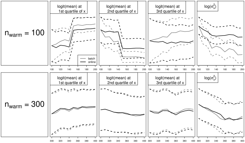
Figure 5: Convergence diagnostics for a binary response nonparametric regression example with data generated according to (19). The solid lines track the posterior means, whilst the dashed lines show corresponding 95% credible sets. First row: the horizontal axes show the sample sizes between a warm-up batch sample of size $n_{\mbox{\scriptsize warm}}=100$ and validation sample sizes up to $n_{\mbox{\scriptsize valid}}=100$ greater than $n_{\mbox{\scriptsize warm}}$. Second row: as for the first row, but with $n_{\mbox{\scriptsize warm}}=300$.

The analogues of Steps 1.-5. of Algorithm 2’ were applied with an initial trial involving $n_{\mbox{\scriptsize warm}}=100$ and $n_{\mbox{\scriptsize valid}}=100$. The Bayes estimates and 95% credible sets of the logit-transformed mean function at each of the quartiles of the $x$-values, as well as $\log(\sigma_{u}^{2})$, are shown in the upper row of Figure 5. However, they have noticeable disagreement, which indicates non-convergence of the online MFVB results to their batch counterparts and that $n_{\mbox{\scriptsize warm}}$ should be increased. Setting $n_{\mbox{\scriptsize warm}}=300$ leads to the more concordant results shown in the lower row of Figure 5, indicating adequacy of this warm-up size. We have found this behaviour typical for binary response online MFVB and this simple example demonstrates the importance of batch-based tuning and convergence diagnostics.

4 Justification for Using Mean Field Variational Bayes

Our use of online mean field variational Bayes is founded upon it being the only approach of which we are aware that (a) is readily extendible to a wide range of semiparametric regression models and (b), in the case of streaming data, has the ability to perform fast approximate inference for all model parameters.

Various other approaches such as stochastic gradient descent, Markov chain Monte Carlo and expectation-maximisation can be ruled out since they fall short on at least one of these criteria. We now provide brief reasoning for their elimination from contention for real-time semiparametric regression.

Stochastic gradient descent (e.g. Zhang, 2004) allows for regularized regression models to be fitted in an online fashion. Recently Langford, Li & Zhang (2009) devised stochastic gradient methodology for sparse signal regression. However, in both Zhang (2004) and Langford et al. (2009), the regularization parameters need to be inputted. This is in contrast to Algorithms 3 and 4 in which the regularization parameters are embedded in the underlying Bayesian model in the form of variance parameters. This allows online estimation of the optimal amount of regularization. It appears that current stochastic gradient descent technology does not support online estimation of regularization parameters.

Markov chain Monte Carlo (MCMC) has analogues with MFVB but is much more computationally expensive. The full conditional distributions depend on the same matrix algebraic forms, such as $\boldsymbol{y}^{T}\boldsymbol{y}$, $\boldsymbol{C}^{T}\boldsymbol{y}$ and $\boldsymbol{C}^{T}\boldsymbol{C}$, that appear in the batch MFVB algorithms for our semiparametric regression models. As shown in Algorithms 3–5, these forms are simple to update whenever a new vector of observations arrives. But MCMC then requires multiple sampling from the resulting full conditional distributions. This is much more expensive than MFVB’s arithmetic updates. For streaming data, this heavy computational burden will tend to rule out MCMC.

Expectation-Maximization (EM) analogues of Algorithm 3, but for frequentist linear mixed models, are given in Sections 14.2a and 14.2b of McCulloch, Searle & Neuhaus (2008). They are similar in nature to batch MFVB algorithms such as Algorithm 3 of Ormerod & Wand (2010) and, therefore, can be readily adapted for online processing. Estimates of the precision are not included and further computing, possibly involving the Louis (1982) methodology, is required for online inference. Moreover, the handling of sparse shrinkage penalties and binary response variables requires considerably more complicated EM algorithms, and require approximation, such as Laplace’s method, to be computationally feasible. In summary, an EM approach may lead to viable real-time semiparametric regression algorithms, but they would be much more complicated than Algorithms 2–5.

Lastly, we mention Newton-Raphson optimization of the likelihood within a frequentist framework (e.g., Section 14.2c of McCulloch, Searle & Neuhaus, 2008). For streaming data, there is the problem of how to keep track of convergence of the Newton-Raphson schemes as data continually arise. The modification for sparse signal penalties looks particularly challenging. The binary response case also involves intractable forms which necessitate approximations such as those based on Laplace’s method.

5 Inferential Accuracy

Algorithms 2–5 perform real-time approximate Bayesian inference for the model parameters. We now discuss the quality of the approximations induced by the mean field assumptions.

Inferential accuracy of MFVB is a relatively new and modestly studied area of statistical research. There have been a few theoretical contributions, such as Wang & Titterington (2005), and simulation studies, such as those presented in Faes, Ormerod & Wand (2011), but considerably more research is needed. For the semiparametric regression models considered in the present article, a broad summary is that MFVB exhibits good to excellent inferential accuracy for the Gaussian response models of Section 2 but only moderate to good accuracy for the binary response model (17). In particular, the approximate posterior density functions produced by Algorithm 5 exhibit good accuracy for the variance parameters. But for the coefficient vectors $\boldsymbol{\beta}$ and $\boldsymbol{u}$ the approximate posterior density functions, whilst exhibiting good locational behaviour, tend to under-approximate the spread.

Recently, Menictas & Wand (2013) provided some heuristic arguments, based on likelihood theory, for why mean field approximations such as (3) and (9) can be highly accurate for Gaussian response models of Section 2. The essential reason is parameter orthogonality between the coefficient parameters and variance parameters.

Improving the accuracy of MFVB-based inference, especially for non-Gaussian response models such as Algorithm 5, is an important problem for future research. For streaming data, a possible approach is to obtain batch MCMC-based fits in the warm-up phase and/or on parallel processors. These more accurate fits could then be used to make appropriate corrections to the online MFVB-based output. However, the details and efficacy of such an approach are yet to be explored.

6 Live Internet Demonstrations

We have launched the web-site: realtime-semiparametric-regression.net for displaying live real-time semiparametric regression analyses. Links on this web-site point to several examples, and we anticipate that the set of examples will grow during the next few years. At the time of this writing, the examples involve simulated data and three types of real-time data: stock prices from the U.S. National Association of Securities Dealers Automated Quotations (NASDAQ) and the London Stock Exchange in the United Kingdom, features of property rentals in Sydney, Australia, and data on delays in U.S. domestic flights.

6.1 Simulated Data

Our lead-off examples involve synthetic data. First consider the Gaussian additive model

$$\begin{array}[]{l}y_{i}|\boldsymbol{\beta},\boldsymbol{u}_{4},\boldsymbol{u}_{5},\boldsymbol{u}_{6},\sigma_{\varepsilon}^{2}\sim N\Big{(}\beta_{1}\,x_{1i}+\beta_{2}\,x_{2i}+\beta_{3}\,x_{3i}\\ \qquad\qquad+f_{4}(x_{4i})+f_{5}(x_{5i})+f_{6}(x_{6i}),\sigma_{\varepsilon}^{2}\Big{)}\end{array}$$ (20)

where, for $j=4,5,6$, $\boldsymbol{u}_{j}$ is vector of spline coefficients for $f_{j}$. We generated 30,000 observations from (20) with $x_{1i},x_{2i},x_{3i}\stackrel{{\scriptstyle{\tiny\mbox{ind.}}}}{{\sim}}\mbox{Bernoulli}\,({\textstyle{\frac{1}{2}}})$ and $x_{4i},x_{5i},x_{6i}\stackrel{{\scriptstyle{\tiny\mbox{ind.}}}}{{\sim}}N(0,1)$. Truth was set according to $\beta_{1}=0.2$, $\beta_{2}=-0.3$, $\beta_{3}=0.6$, $f_{4}(x)=2\Phi(6x-3)$, $f_{5}(x)=\sin(3\pi x^{3})$, $f_{6}(x)=\cos(4\pi x)$ and $\sigma_{\varepsilon}^{2}=1$. The link Gaussian additive model on the abovementioned web-site points to a movie showing summaries of the regression fits when the data are sequentially fed into Algorithm 3.

The Logistic additive model link points to a similar movie, but with data generated from the logistic additive model

$$y_{i}\,|\,\boldsymbol{\beta},\boldsymbol{u}_{2},\boldsymbol{u}_{3}\sim\mbox{Bernoulli}\big{(}\mbox{logit}^{-1}(\beta_{1}\,x_{1i}+f_{2}(x_{2i})+f_{3}(x_{3i}))\big{)}$$

with $x_{1i}\stackrel{{\scriptstyle{\tiny\mbox{ind.}}}}{{\sim}}\mbox{Bernoulli}\,({\textstyle{\frac{1}{2}}})$, $x_{2i},x_{3i}\stackrel{{\scriptstyle{\tiny\mbox{ind.}}}}{{\sim}}N(0,1)$ and truth set at $\beta_{1}=0.2$, $f_{2}(x)=\cos(4\pi\,x)+2\,x$ and $f_{3}(x)=\sin(2\pi\,x^{2})$.

Lastly, the Wavelet regression link corresponds to the simulation setting used to produce Figure 4, with description given in Section 2.4.

6.2 Stock Price Data

In this set of examples, the predictor and response variable pairs correspond to pairs of stock prices. An example nonparametric regression model is

$$(\mbox{{Microsoft\,\,stock\,\,price}})_{i}|\,\boldsymbol{\beta},\boldsymbol{u},\sigma_{\varepsilon}^{2}\stackrel{{\scriptstyle{\tiny\mbox{ind.}}}}{{\sim}}N(\beta_{0}+f(\mbox{{(Intel\,\,stock\,\,price)}}_{i}),\sigma_{\varepsilon}^{2})$$ (21)

where $f(x)=\beta_{1}\,x+\sum_{k=1}^{K}\,u_{k}\,z_{k}(x)$ is a penalized spline function as described in Section 2.2 with the same distributional structures imposed on the model parameters. In addition, $(\mbox{{Microsoft stock price}})_{i}$ and $(\mbox{{Intel}}$ $\mbox{{stock price}})_{i}$ denote the $i$th stock price for the U.S. companies Microsoft Corporation and Intel Corporation, respectively, for the current trading day. The web-site displays fitting of (21) in real-time during the NASDAQ opening hours (9:30am to 4:00pm North American Eastern Standard Time). The R package quantmod (Ryan, 2012) is used to obtain the NASDAQ data from the Yahoo! Finance web-site (finance.yahoo.com).

A similar series of examples is set up using London Stock Exchange data during stock market opening hours (8:00 am to 4:20 pm Greenwich Mean Time). Note that Yahoo! Finance delays London Stock Exchange data by 20 minutes.

Depending on the example and the live data-set, the appropriateness of the nonparametric regression model (21) may be questionable and more sophisticated models could be entertained. Hence, these examples should only be viewed as simple illustrations of the concept of real-time semiparametric regression.

6.3 Sydney Property Rental Data

This example involves real-time semiparametric regression analysis of data from the property rental market in Sydney, Australia. Each day, hundreds of properties come on the Sydney market and these fresh data are usually advertised on rental agency web-sites and real estate web-sites as realestate.com.au. This offers the possibility to perform real-time analysis and produce live and up-to-date summaries of the rental market status. An attractive approach to model such data is the special case of semiparametric regression known as geoadditive models (Kammann and Wand, 2003). Explicitly, we work with the model

$$\begin{array}[]{l}\log((\mbox{{weekly\,\,rent}})_{ij})|\,\boldsymbol{\beta},U_{i},\boldsymbol{u}_{2},\boldsymbol{u}_{3},\boldsymbol{u}_{4},\boldsymbol{u}_{5},\sigma_{\varepsilon}^{2}\stackrel{{\scriptstyle{\tiny\mbox{ind.}}}}{{\sim}}\\[4.30554pt] \qquad N(\beta_{0}+\beta_{1}\,\mbox{{house}}_{ij}+f_{2}(\mbox{{(number\,\,of\,\,bedrooms)}}_{ij})\\[4.30554pt] \qquad+f_{3}(\mbox{{(number\,\,of\,\,bathrooms)}}_{ij})+f_{4}(\mbox{{(number\,\,of\,\,car\,\,spaces)}}_{ij})\\[4.30554pt] \qquad+f_{5}(\mbox{{longitude}}_{ij},\mbox{{latitude}}_{ij})+U_{i},\sigma_{\varepsilon}^{2}),\hbox{}\qquad U_{1},\ldots,U_{992}|\,\sigma_{U}^{2}\stackrel{{\scriptstyle{\tiny\mbox{ind.}}}}{{\sim}}N(0,\sigma_{U}^{2}).\end{array}$$ (22)

Here, $\mbox{({weekly rent})}_{ij}$ is the weekly rental amount in Australian dollars of the $j$th property for the $i$th real estate agency (hereafter called the $(i,j)$th property), and $\mbox{{house}}_{ij}$ is an indicator of the $(i,j)$th property being a house, townhouse or villa (rather than an apartment). The variable $\mbox{{(number\,\,of\,\,bedrooms)}}_{ij}$ is the number of bedrooms in the $(i,j)$th property. Variables concerning the numbers of bathrooms and car spaces are defined similarly. The geographical location of the $(i,j)$th property is conveyed by the variables $\texttt{longitude}_{ij}$ and $\texttt{latitude}_{ij}$. The $U_{i}$, $1\leq i\leq 992$, are random intercepts for each of the 992 agencies. The fixed effect regression coefficients $\beta_{0}$, $\beta_{1}$ and the linear contribution to $f_{2},\ldots,f_{5}$ are stored in $\boldsymbol{\beta}$. Similarly, the spline basis coefficients for $f_{2},\ldots,f_{5}$ are stored in $\boldsymbol{u}_{2},\ldots,\boldsymbol{u}_{5}$. The estimate of $f_{5}$ is based on bivariate thin plate splines as explained in Chapter 13 of Ruppert, Wand & Carroll (2003).

The web-site for this example displays fitting of (22) in real time based on data collected since 9th May, 2012. Several regression summaries are presented. Firstly, a geographical map is listed with processed properties as small black dots and recently (i.e. during the last hour) added ones as yellow circles. The total number of processed properties is included at the bottom right. Next, a color-coded geographical map displays the weekly rent for a two bedroom apartment with one bathroom and one car space for various geographical locations. The approximate posterior density function for $\beta_{1}$ shows the impact of the property being a house or not. Regression fits and 95% credible sets for the number of bedrooms, bathrooms and car spaces for apartments are presented. Finally, a list of rental agencies with the least and most expensive properties, after correcting for all other covariates, is provided. All these regression summaries are computed in real time and the figures are updated every hour.

6.4 U.S. Domestic Flight Data

Air traffic delays represent a critical problem for both airlines and passengers. In this section we will demonstrate the proposed methodology for real-time analysis of U.S. domestic flights. We use the web-site www.flightstats.com to obtain real-time data on flight delay, flight distance, operating airline and flight path. Data on temperature, wind speed and aviation flight category is obtained through the aviationweather.gov web-site. This example is inspired by a recent competition, titled GE Flight Quest, run by the kaggle platform (www.kaggle.com).

The real-time data consist of flight delay, flight distance, operating airline and flight path. In addition, data on temperature, wind speed and aviation flight category are available The aviation flight categories are based on the North American conventions known as METAR and are based on the ceiling (height above ground of the base of the lowest layer of cloud) and visibility. Table 1 provides the aviation flight categories definitions.

category	ceiling	and/or visibility
visual flight rules	above 3,000 feet	above 5 miles
marginal visual flight rules	1000–3,000 feet	3–5 miles
instrument flight rules	500–1,000 feet	1–3 miles
low instrument flight rules	below 500 feet	below 1 mile

Table 1: Definitions of North American aviation flight categories.

Our demonstration uses the semiparametric regression model:

$$\begin{array}[]{l}\log(\mbox{{delay}}_{ijk}+120)|\,\boldsymbol{\beta},U_{i},V_{j},\boldsymbol{u}_{7},\boldsymbol{u}_{8},\boldsymbol{u}_{9},\boldsymbol{u}_{10},\boldsymbol{u}_{11},\sigma_{\varepsilon}^{2}\stackrel{{\scriptstyle{\tiny\mbox{ind.}}}}{{\sim}}\\[4.30554pt] \hskip 5.69054ptN(\beta_{0}+\beta_{1}{\mbox{{MVFRdep}}}_{ijk}+\beta_{2}{\mbox{{IFRdep}}}_{ijk}+\beta_{3}{\mbox{{LIFRdep}}}_{ijk}+\beta_{4}{\mbox{{MVFRarr}}}_{ijk}\\[4.30554pt] \hskip 5.69054pt+\beta_{5}{\mbox{{IFRarr}}}_{ijk}+\beta_{6}{\mbox{{LIFRarr}}}_{ijk}+f_{7}({\mbox{{(flight distance)}}}_{j})\\[4.30554pt] \hskip 5.69054pt+f_{8}({\mbox{{(departure temperature)}}}_{ijk})+f_{9}({\mbox{{(arrival temperature)}}}_{ijk})\hbox{}\\[4.30554pt] \hskip 5.69054pt+f_{10}({\mbox{{(departure wind speed)}}}_{ijk})+f_{11}({\mbox{{(arrival wind speed)}}}_{ijk})\hbox{}\\[4.30554pt] \hskip 5.69054pt+U_{i}+V_{j},\sigma_{\varepsilon}^{2}),\hskip 8.53581ptU_{1},\ldots,U_{171}|\,\sigma^{2}_{U}\stackrel{{\scriptstyle{\tiny\mbox{ind.}}}}{{\sim}}N(0,\sigma^{2}_{U}),\hskip 8.53581ptV_{1},\ldots,V_{2,000}|\,\sigma^{2}_{V}\stackrel{{\scriptstyle{\tiny\mbox{ind.}}}}{{\sim}}N(0,\sigma^{2}_{V}).\end{array}$$ (23)

Here delay_ijk is the difference between the actual and scheduled runway arrival time in minutes for the $k$th flight of airline $i$ on flight path $j$ and

$$\texttt{MVFRdep}_{ijk}=\left\{\begin{array}[]{ll}1&\mbox{if marginal visual flight rules apply at the scheduled runway }\\ &\mbox{departure time of the $k$th flight of airline $i$ on flight path $j$}\\ 0&\mbox{otherwise.}\end{array}\right.$$

The variable $\texttt{MVFRarr}_{ijk}$ is defined analogously, but for the scheduled runway arrival time. The other aviation flight category variables are defined similarly, with IFR denoting “instrument flight rules” and LIFR denoting “low instrument flight rules”. The variable (flight distance)_j denotes the distance of flight path $j$ in kilometers. Variables (departure temperature)_ijk and (arrival temperature)_ijk are the temperature in degrees Celsius at the scheduled runway departure and arrival time of the $k$th flight of airline $i$ on flight path $j$, respectively. Variables (departure wind speed)_ijk and (arrival wind speed)_ijk are the wind speed in knots at the scheduled runway departure and arrival time of the $k$th flight of airline $i$ on flight path $j$, respectively. The $U_{i}$,$1\leq i\leq 171$, are random intercepts for each of the 171 airlines, while $V_{j}$,$1\leq j\leq$ 2,000, are random effects for each of the 2,000 flight paths. The fixed effect regression coefficients $\beta_{0},\ldots,\beta_{6}$ and the linear contribution to $f_{7},\ldots,f_{11}$ are stored in $\boldsymbol{\beta}$. Similarly, the spline basis coefficients for $f_{7},\ldots,f_{11}$ are stored in $\boldsymbol{u}_{7},\ldots,\boldsymbol{u}_{11}$.

The link U.S. domestic flight data on our live demonstrations web-site displays fitting of (23) in real time based on data collected since 25th January, 2013. A map shows the flight paths that have most recently been processed and the number of processed flights is given at the bottom of the map. Various regression summaries are provided. Of particular interest are tables of airlines and flight paths with the lowest and highest delays. All these regression summaries are computed in real-time and the figures are updated every few minutes.

References

Albert, J.H. & Chib, S. (1993). Bayesian analysis of binary and polychotomous response data. Journal of the American Statistical Association, 88, 669–679.

Armagan, A., Dunson, D.B. & Lee, J. (2012). Generalized double Pareto shrinkage. Statistica Sinica, to appear.

Bishop, C.M. (2006). Pattern Recognition and Machine Learning. New York: Springer.

Cameron, A.C. & Trivedi, P.K. (2005). Microeconometrics: Methods and Applications. New York: Cambridge University Press.

Carvalho, C.M., Polson, N.G. & Scott, J.G. (2010). The horseshoe estimator for sparse signals. Biometrika, 97, 465–480.

Consonni, G. & Marin, J.-M. (2007). Mean-field variational approximate Bayesian inference for latent variable models. Computational Statistics and Data Analysis, 52, 790–798.

Croissant, Y. (2011). Ecdat 0.1. Data sets for econometrics. R package,
cran.r-project.org

Devroye, L. & Wagner, T.J. (1980). On the $L_{1}$ convergence of kernel estimators of regression functions with application to discrimination. Zeitschrift für Wahrscheinlichkeitstheorie und Vervandte Gebiete, 51, 15–25.

Faes, C., Ormerod, J.T. & Wand, M.P. (2011). Variational Bayesian inference for parametric and nonparametric regression with missing data. Journal of the American Statistical Association, 106, 959–971.

Fricker, R.D. & Chang, J.T. (2008). A spatio-temporal methodology for real-time biosurveillance. Quality Engineering, 20, 465–477.

Girolami, M. & Rogers, S. (2006). Variational Bayesian multinomial probit regression. Neural Computation, 18, 1790–1817.

Gradshteyn, I.S. & Ryzhik, I.M. (1994). Tables of Integrals, Series, and Products, 5th Edition, San Diego, California: Academic Press.

Griffin, J.E. & Brown, P.J. (2011). Bayesian hyper lassos with non-convex penalization. Australian and New Zealand Journal of Statistics, 53, 423–442.

Härdle, W. (1990). Applied Nonparametric Regression. Cambridge: Cambridge University Press.

Hoffman, M., Blei, D. & Bach, F. (2010). Online learning for latent Dirichlet allocation. In Advances in Neural Information Processing Systems 23, Lafferty, J., Williams, C.K.I., Shawe-Taylor, J., Zemel, R.S. & Culotta, A. (eds.) pp. 856–864.

Huang, A. & Wand, M.P. (2012). Simple marginally noninformative prior distributions for covariance matrices. Under revision for Bayesian Analysis.
www.uow.edu/$\sim\,$mwand/papers.html

Jaakkola, T.S. & Jordan, M.I. (2000). Bayesian parameter estimation via variational methods. Statistics and Computing 10, 25–37.

Jank, W. & Shmueli, G. (2007). Modelling concurrency of events in on-line auctions via spatiotemporal semiparametric models. Applied Statistics, 56, 1–27.

Johnstone, I.M. & Silverman, B.W. (2005). Empirical Bayes selection of wavelet thresholds. The Annals of Statistics, 33, 1700–1752.

Kaimi, I. & Diggle, P.J. (2011). A hierarchical model for real-time monitoring of variation in risk of non-specific gastro-intestinal infections. Epidemiology and Infection, 139, 1854–1862.

Kammann, E.E. and Wand, M.P. (2003). Geoadditive models. Journal of the Royal Statistical Society, Series C, 52, 1–18.

Krzyzak, A. & Pawlak, M. (1984). Almost everywhere convergence of a recursive regression function estimate and classification. IEEE Transactions on Information Theory, IT-30, 91–93.

Langford, J., Li, L. & Zhang, T. (2009). Sparse online learning via truncated gradient. Journal of Machine Learning Research, 10, 777–801.

Louis, T.A. (1982). Finding the observed information matrix when using the EM algorithm. Journal of the Royal Statistical Society, Series B, 44, 226–233.

Luenberger, D.G. & Ye, Y. (2008). Linear and Nonlinear Programming. New York: Springer, 3rd edition.

McCulloch, C.E., Searle, S.R. & Neuhaus, J.M. (2008). Generalized, Linear, and Mixed Models, 2nd Edition. John Wiley & Sons, New York.

Menictas, M. & Wand, M.P. (2013). Variational inference for marginal longitudinal semiparametric regression. Stat, in press.

Michalak, S., DuBois, A., DuBois, D., Vander Wiel, S. & Hogden, J. (2012). Developing systems for real-time streaming analysis. Journal of Computational and Graphical Statistics, 21, 561–580.

Neville, S.E., Ormerod, J.T. & Wand, M.P. (2012). Mean field variational Bayes for continuous sparse signal shrinkage: pitfalls and remedies.
www.uow.edu/$\sim\,$mwand/papers.html

Ng, S-K., McLachlan, G.J. & Lee, A.H. (2006). An incremental EM-based learning approach for on-line prediction of hospital resource utilization. Artificial Intelligence in Medicine, 36, 257–267.

Ormerod, J.T. & Wand, M.P. (2010). Explaining variational approximations. The American Statistician, 64, 140–153.

Ruppert, D., Wand, M.P. & Carroll, R.J. (2003). Semiparametric Regression. New York: Cambridge University Press.

Ruppert, D., Wand, M.P. & Carroll, R.J. (2009). Semiparametric regression during 2003-2007. Electronic Journal of Statistics, 3, 1193–1256.

Ryan, J.A. (2012) quantmod 0.3. Quantitative financial modelling framework. R package,
cran.r-project.org

Smith, A.D.A.C. & Wand, M.P. (2008). Streamlined variance calculations for semiparametric mixed models. Statistics in Medicine, 27, 435–448.

Tchumtchoua, S., Dunson, D.B. & Morris, J.S. (2012). Online variational Bayes inference for high-dimensional correlated data. Unpublished manuscript.
www.stat.duke.edu/$\sim\,$dunson/submitted.html

Wainwright, M.J. & Jordan, M.I. (2008). Graphical models, exponential families, and variational inference. Foundation and Trends in Machine Learning, 1, 1–305.

Wand, M.P. (2009). Semiparametric regression and graphical models. Australian and New Zealand Journal of Statistics, 51, 9–41.

Wand, M.P. & Jones, M.C. (1995) Kernel Smoothing. London: Chapman and Hall.

Wand, M.P. & Ormerod, J.T. (2008). On semiparametric regression with O’Sullivan penalized splines. Australian and New Zealand Journal of Statistics, 50, 179–198.

Wand, M.P. & Ormerod, J.T. (2011). Penalized wavelets: embedding wavelets into semiparametric regression. Electronic Journal of Statistics, 5, 1654–1717.

Wang, C., Paisley, J. & Blei, D.M. (2011). Online variational inference for the hierarchical Dirichlet process. International Conference on Artificial Intelligence and Statistics, 2011, Fort Lauderdale, Florida, USA.

Wang, B. & Titterington, D.M. (2005). Inadequacy of interval estimates corresponding to variational Bayesian approximations. In Proceedings of the 10th International Workshop on Artificial Intelligence, eds. R.G. Cowell and Z. Ghahramani, Barbados: Society for Artificial Intelligence and Statistics, pp. 373–380.

Welham, S.J., Cullis, B.R., Kenward, M.G. & Thompson, R. (2007). A comparison of mixed model splines for curve fitting. Australian and New Zealand Journal of Statistics, 49, 1–23.

Wolverton, C.T. & Wagner, T.J. (1969). Asymptotically optimal discriminant functions for pattern recognition. IEEE Transactions on Information Theory, IT-15, 258–265.

Wood, S.N. (2006). Generalized Additive Models: An Introduction with R. Boca Raton, Florida: Chapman & Hall/CRC.

Yamato, H. (1971). Sequential estimation of a continuous probability density function and model. Bulletin of Mathematical Statistics, 14, 1–12.

Zhang, T. (2004). Solving large scale linear prediction problems using stochastic gradient descent algorithms. In Proceedings of the Twenty-First International Conference on Machine Learning, Brodley, C.E. (ed.). pp. 919–926.

Zhao, Y., Staudenmayer, J., Coull, B.A. & Wand, M.P. (2006). General design Bayesian generalized linear mixed models. Statistical Science, 21, 35–51.