Finite temperature dynamical properties of SU($N$) fermionic Hubbard models in the spin-incoherent regime

Abstract

We study strongly correlated Hubbard systems extended to symmetric $N$-component fermions. We focus on the intermediate-temperature regime between magnetic superexchange and interaction energy, which is relevant to current ultracold fermionic atom experiments. The $N$-component fermions are represented by slave particles, and, by using a diagrammatic technique based on the atomic limit, spectral functions are analytically obtained as a function of temperature, filling factor and the component number $N$. We also apply this analytical technique to the calculation of lattice modulation experiments. We compute the production rate of double occupancy induced by modulation of an optical lattice potential. Furthermore, we extend the analysis to take into account the trapping potential by use of the local density approximation. We find an excellent agreement with recent experiments on ¹⁷³Yb atoms.

I Introduction

The realization of ultracold atoms in an optical lattice opens up the possibility to study in a controlled way strongly correlated quantum systems Esslinger (2010); Bloch et al. (2008). Such strongly correlated atoms are well described by the Hubbard model. This model plays a central role for the study of the Mott insulator (MI) transition Imada et al. (1998), high-$T_{c}$ superconductivity Lee et al. (2006), and quantum magnetism. In addition, the high controllability of model parameters such as the interaction by a Feshbach resonance technique and kinetic energy by changing the lattice depth allows us to capture such Hubbard physics in a broad range of parameter regimes.

The recent achievement of Fermi degeneracy of ultracold alkaline-earth-metal(-like) atoms such as ⁴³Ca, ⁸⁷Sr, and ¹⁷³Yb potentially provides a new class of strongly correlated matter. The structure of their nuclear spin degrees of freedom allows the realization of high symmetry groups for the internal degree of freedom (“spin”). For instance, ¹⁷³Yb atoms behave as a spin-$5/2$ fermion Taie et al. (2010); Fukuhara et al. (2007); Cazalilla et al. (2009) and ⁸⁷Sr as a spin-$9/2$ fermion Ye et al. (2008); Hermele et al. (2009, 2011); DeSalvo et al. (2010). In particular, provided all $s$-wave scattering lengths are independent of the atomic spin states, the atom cloud as a many-body system obeys high symmetries. Thus the confinement of alkaline-earth-metal(-like) atoms in an optical lattice provides opportunities for the study of the SU($N$) symmetric Hubbard model for spin-$(N-1)/2$ atoms. The experimental realization of such SU($N$) Hubbard models has strongly stimulated the corresponding theoretical studies  Hermele et al. (2009, 2011); Manmana et al. (2011); Honerkamp and Hofstetter (2004); Cazalilla et al. (2009); Gorshkov et al. (2010); Hazzard et al. (2012); Nonne et al. (2010, 2011a, 2011b); Azaria et al. (2009).

In condensed matter physics, the SU($N$) symmetric systems have been introduced as a purely theoretical extension of the strongly correlated electron systems with SU($2$) spin rotational symmetry, e.g., for quantum magnetism Arovas and Auerbach (1988); Read and Sachdev (1989, 1990); Harada et al. (2003); Kawashima and Tanabe (2007) or for the Hubbard model  Ruckenstein and Schmitt-Rink (1988) in the context of high-$T_{c}$ superconductivity Affleck and Marston (1988); Marston and Affleck (1989); Lavagna et al. (1987); Kotliar and Liu (1988). As a theoretical tool to solve such problems, the slave-particle technique, originally developed for the single impurity Anderson model Abrikosov (1965); Barnes (1976); Read and Newns (1983); Coleman (1984), has been used and applied to the Hubbard model Kotliar and Ruckenstein (1986); Li et al. (1989); Lavagna (1990); Kane et al. (1989); Marsiglio et al. (1991). More recently, the slave-boson approach has also been used with success in the cold atom context Sensarma et al. (2009); Huber and Rüegg (2009); Tokuno et al. (2012).

In this paper, we generalize the slave-boson calculation scheme introduced in Ref. Tokuno et al. (2012) to the symmetric $N$-component fermionic atom systems including SU($N$) symmetry. This technique has proven an effective way to compute the dynamics of strongly interacting systems at a filling of one or less than one particle per site in the spin-incoherent temperature regime for which the temperature is lower than the interaction energy, but larger than the magnetic superexchange one. This regime is directly relevant to the current experiments on fermionic atoms. A diagrammatic approach based on the noncrossing approximation (NCA) with the spin-incoherent assumption is used to estimate self-energies and compute the spectral functions as functions of temperature, chemical potential, and component number $N$. This allows us in particular to compare the physics for different $N$s.

We also use these techniques to compute the effect of lattice modulation spectroscopy which has been recently implemented in experiments. The lattice modulation technique has been originally applied to bosonic atom systems, in which the absorbed energy is measured as a function of the modulation frequency Stöferle et al. (2004). According to the linear response formalism, the energy absorption rate in such a weak perturbation regime gives access to the kinetic-energy correlation functions Iucci et al. (2006); Reischl et al. (2005); Kollath et al. (2006). For fermionic atoms, an accurate measurement of the absorption energy is difficult, and a variant of the probe measuring the production rate of so-called doublons, which is the number of doubly occupied sites, induced by the lattice modulation has been proposed. Kollath et al. (2006) The doublon production rate (DPR) has been shown to be identical to the energy absorption rate both numerically and analytically Kollath et al. (2006); Tokuno and Giamarchi (2011, 2012). This doublon measurement technique has been successfully implemented in a fermionic atom experiment Jördens et al. (2008). This allowed more recent experiments to successfully reach the linear response regime for which the DPR spectrum scales quadratically with the modulation amplitude. Greif et al. (2011) A direct comparison with equilibrium theory is possible and has been successfully done Sensarma et al. (2009); Tokuno et al. (2012). So far the lattice modulation experiment has been done with ⁴⁰K Greif et al. (2011) behaving as a spin-$1/2$ fermion and ¹⁷³Yb Taie et al. (2012) behaving as a spin-$5/2$ fermion.

The paper is organized as follows. In Sec. II, we introduce the Hubbard model for the $N$-component fermions which includes SU($N$) symmetry. The introduced Hamiltonian is rewritten in a slave-particle representation. In Sec. III, we discuss the single particle properties based on the Hubbard Hamiltonian using this slave-particle representation. Then, using a diagrammatic approach starting from the atomic limit, self-consistent equations of doublon and holon self-energies are constructed and solved analytically. In Sec. IV, using the spectral functions given in Sec. III, we investigate the DPR spectrum produced by an amplitude modulation of the optical lattice potential. Then the analytic form of the DPR spectrum is given. In addition, we extend the calculation to the trapped case by using the local density approximation (LDA), and we also compare our results to the recent experiment with ¹⁷³Yb atoms. Finally, our results are summarized in Sec. V. Some technical details on the formulation of the DPR spectrum are briefly reviewed in Appendix A.

II Model

II.1 SU($N$)-symmetric Hubbard model

In lattice systems with multicomponent particles, multiparticle occupation states in addition to double occupancy can be defined in general. However, when the interaction between different components is strong, such multiple-occupation is at a higher energy state than double occupancy. Because we are interested in physics of doublon excitations at a filling of one or less than one particle per site, such higher occupation states are way above the main energy scale of interest. Thus, as an effective model Hamiltonian, we can extend the Hubbard type two-body interaction to the $N$-component case. Then interactions between different components, determined by the $s$-wave scattering lengths, generally take different values depending on the components: The interaction parameter is written as $U_{\sigma,\sigma^{\prime}}$ where $\sigma$ and $\sigma^{\prime}$ are the indices characterizing the internal state of the fermions. We consider the special case of a unique interaction parameter, $U_{\sigma,\sigma^{\prime}}=U$ Kitagawa et al. (2008); Stellmer et al. (2011); namely the coupling does not depend on the components.  Then, the interaction term has the same symmetry as the kinetic term, and the system symmetry turns out to be enlarged to SU($N$) symmetry.

We consider the generalized $N$-component fermionic Hubbard model, $H=H_{\rm K}+H_{\rm at}$ with

$$H_{\rm K} =-J\sum_{\sigma=1}^{N}\sum_{\langle{i,j}\rangle}c^{\dagger}_{i,\sigma}c_{j,\sigma},$$ (1)

$$H_{\rm at} =-\mu\sum_{\sigma=1}^{N}\sum_{j}n_{j,\sigma}+\sum_{\sigma\neq\sigma^{\prime}}\sum_{j}\frac{U}{2}n_{j,\sigma}n_{j,\sigma^{\prime}},$$

where $c_{j,\sigma}$ is the annihilation operator of a fermion with the internal component $\sigma$ at a site $j$, and $n_{j,\sigma}$ is the number operator. The parameters $J$ and $U$, respectively, denote the nearest-neighbor hopping energy and the on-site interaction between components $\sigma$ and $\sigma^{\prime}$. Throughout this paper, we consider only the repulsive case $U>0$.

In the considered regime of chemical potentials, particle-hole symmetry always disappears except for the $N=2$ case at $\mu=U/2$. This is because for $N>2$ there are $N(N-1)/2$ doublon states while the hole state is unique.

II.2 slave particle representation

The $N$-component fermions have a larger Hilbert space than that of the two-component case: While an empty site (holon) is unique, there exist multiple-occupation states (three- and four-fold occupation, and so on) in addition to $N(N-1)/2$-species doubly occupied states (doublons) and $N$-species single occupied spin states (spinons). The multiple-occupation states are energetically out of shell, since those states cost an energy higher than $2U$, which is over the energetic cutoff in our model Hamiltonian. Thus in our case we describe the single-site state by a holon $\ket{h}$, $N$-species spinon $\ket{\sigma}$ ($\sigma=1,2,\cdots,N$), and $N(N-1)/2$-species doublons $\ket{d_{\sigma,\sigma^{\prime}}}$ ($\sigma\neq\sigma^{\prime}$ and $\sigma,\sigma^{\prime}=1,\cdots,N$). In terms of doublon states, the antisymmetrization condition $\ket{d_{\sigma,\sigma^{\prime}}}=-\ket{d_{\sigma^{\prime},\sigma}}$ is imposed. We hereafter suppose that the spin indices in $\ket{d_{\sigma,\sigma^{\prime}}}$ are ordered such that $\sigma>\sigma^{\prime}$. The single-site original fermionic operators, $c_{\sigma}$ and $c_{\sigma}^{\dagger}$, are given by

$$c_{\sigma} =\ket{h}\bra{\sigma}+\sum_{\sigma^{\prime}=1}^{\sigma-1}\ket{\sigma^{\prime}}\bra{d_{\sigma,\sigma^{\prime}}}-\sum_{\sigma^{\prime}=\sigma+1}^{N}\ket{\sigma^{\prime}}\bra{d_{\sigma^{\prime},\sigma}},$$ (2)

$$c_{\sigma}^{\dagger} =\ket{\sigma}\bra{h}+\sum_{\sigma^{\prime}=1}^{\sigma-1}\ket{d_{\sigma^{\prime},\sigma}}\bra{\sigma^{\prime}}-\sum_{\sigma^{\prime}=\sigma+1}^{N}\ket{d_{\sigma,\sigma^{\prime}}}\bra{\sigma^{\prime}}.$$ (3)

Then the representation no longer gives back the anticommutation relation $\{c_{\sigma},c_{\sigma}^{\dagger}\}=\delta_{\sigma,\sigma^{\prime}}$, but it should be approximately correct as long as $U$ is much larger than the particle hopping $J$ and temperature, and the filling is less than unity, which means that all the excitations leave the system in the proper subpart of the Hilbert space. We introduce the creation and annihilation operators for a holon, spinons, and doublons as

$$\ket{\sigma}\bra{h}=b_{\sigma}^{\dagger}h,$$ (4)

$$\ket{h}\bra{\sigma}=h^{\dagger}b_{\sigma},$$

$$\ket{d_{\sigma,\sigma^{\prime}}}\bra{\sigma^{\prime\prime}}=d_{\sigma\sigma^{\prime}}^{\dagger}b_{\sigma^{\prime\prime}},$$

$$\ket{\sigma^{\prime\prime}}\bra{d_{\sigma,\sigma^{\prime}}}=b_{\sigma^{\prime\prime}}^{\dagger}d_{\sigma\sigma^{\prime}},$$

and the new vacuum state $\ket{0}$ is defined as $b_{\sigma}\ket{0}=h\ket{0}=d_{\sigma\sigma^{\prime}}\ket{0}=0$.

It is easy to extend the above single-site argument to multi-site problems: All operators become site dependent. In order to recover the anticommutation relations between the original fermions at different sites, $\{c_{i,\sigma},c_{j,\sigma^{\prime}}^{\dagger}\}=0$ ($i\neq j$), we assume the following commutation and anticommutation relations: $\{h_{i},h_{j}^{\dagger}\}=\delta_{i,j}$, $\{d_{i,\sigma\sigma^{\prime}},d_{j,\eta\eta^{\prime}}^{\dagger}\}=\delta_{i,j}\delta_{\sigma,\eta}\delta_{\sigma^{\prime},\eta^{\prime}}$, and $[b_{i,\sigma},b_{j,\sigma^{\prime}}^{\dagger}]=\delta_{i,j}\delta_{\sigma,\sigma^{\prime}}$. Furthermore, by imposing the following constraint we project onto the physical subspace the Hilbert space enlarged by introducing the holon, spinons, and doublons:

$$h_{j}^{\dagger}h_{j}+\sum_{\sigma=1}^{N}b_{j,\sigma}^{\dagger}b_{j,\sigma}+\sum_{\sigma>\sigma^{\prime}}d_{j,\sigma\sigma^{\prime}}^{\dagger}d_{j,\sigma\sigma^{\prime}}=1,$$ (5)

which means that the double occupation on the same site by the slave particles (holon, spinons and doublons) is forbidden.

In summary, the $N$-component fermion in the reduced Hilbert space where the multiple-occupied states are truncated is described in slave particle description as follows:

$$c_{j,\sigma} =h_{j}^{\dagger}b_{j,\sigma}+\sum_{\sigma^{\prime}=1}^{\sigma-1}b_{j,\sigma^{\prime}}^{\dagger}d_{j,\sigma\sigma^{\prime}}-\sum_{\sigma^{\prime}=\sigma+1}^{N}b_{j,\sigma^{\prime}}^{\dagger}d_{j,\sigma^{\prime}\sigma},$$ (6)

$$c_{j,\sigma}^{\dagger} =b_{j,\sigma}^{\dagger}h_{j}+\sum_{\sigma^{\prime}=1}^{\sigma-1}d_{j,\sigma\sigma^{\prime}}^{\dagger}b_{j,\sigma^{\prime}}-\sum_{\sigma^{\prime}=\sigma+1}^{N}d_{j,\sigma^{\prime}\sigma}^{\dagger}b_{j,\sigma^{\prime}}.$$

Due to the slave-particle constraint (5) this representation automatically leads to the expected number operator:

$$n_{j\sigma}=b_{j,\sigma}^{\dagger}b_{j,\sigma}+\sum_{\sigma^{\prime}=1}^{\sigma-1}d_{j,\sigma\sigma^{\prime}}^{\dagger}d_{j,\sigma\sigma^{\prime}}+\sum_{\sigma^{\prime}=\sigma+1}^{N}d_{j,\sigma^{\prime}\sigma}^{\dagger}d_{j,\sigma^{\prime}\sigma}.$$ (7)

The constraint (5) is imposed by a Lagrange multiplier method. The Hamiltonian (1) is represented as

$$H_{\mathrm{K}} =-J\sum_{\langle{i,j}\rangle}\Biggl{[}\sum_{\sigma=1}^{N}\mathcal{F}_{i,j}^{\sigma\sigma}h_{i}h_{j}^{\dagger}+\sum_{\sigma_{1}>\sigma_{2}}\biggl{(}\mathcal{A}_{i,j}^{\sigma_{1}\sigma_{2}\dagger}h_{i}d_{j,\sigma_{1}\sigma_{2}}$$

$$\quad+\mathcal{F}_{j,i}^{\sigma_{2}\sigma_{2}}d_{i,\sigma_{1}\sigma_{2}}^{\dagger}d_{j,\sigma_{1}\sigma_{2}}+\mathrm{H.c.}\biggr{)}$$

$$\quad+\sum_{\sigma_{1}>\sigma_{2}>\sigma_{3}}\biggl{(}\mathcal{F}_{j,i}^{\sigma_{3}\sigma_{2}}d_{i,\sigma_{1}\sigma_{2}}^{\dagger}d_{j,\sigma_{1}\sigma_{3}}$$

$$\quad+\mathcal{F}_{j,i}^{\sigma_{2}\sigma_{1}}d_{i,\sigma_{1}\sigma_{3}}^{\dagger}d_{j,\sigma_{2}\sigma_{3}}-\mathcal{F}_{j,i}^{\sigma_{1}\sigma_{3}}d_{i,\sigma_{2}\sigma_{3}}^{\dagger}d_{j,\sigma_{1}\sigma_{2}}$$

$$\quad+\mathrm{H.c.}\biggr{)}\Biggr{]},$$ (8)

$$H_{\mathrm{at}} =\sum_{j}\biggl{[}-\mu-\lambda_{j}+\epsilon_{j}^{\mathrm{h}}h_{j}^{\dagger}h_{j}+\sum_{\sigma=1}^{N}\epsilon_{j}^{\mathrm{b}}b_{j,\sigma}^{\dagger}b_{j,\sigma}$$

$$\quad+\sum_{\sigma>\sigma^{\prime}}\epsilon_{j}^{\mathrm{d}}d_{j,\sigma\sigma^{\prime}}^{\dagger}d_{j,\sigma\sigma^{\prime}}\biggr{]},$$ (9)

where the local potentials for the slave particles have been introduced as

$$\epsilon_{j}^{\mathrm{h}}=\mu+\lambda_{j},$$ (10)

$$\epsilon_{j}^{\mathrm{b}}=\lambda_{j},$$

$$\epsilon_{j}^{\mathrm{d}}=U-\mu+\lambda_{j},$$

for the holon, spinons and doublons, respectively. $\lambda_{j}$ is the Lagrange multiplier for the local constraint. To simplify the form of $H_{\mathrm{K}}$, a spinon hopping operator from $i$th to $j$th site, $\mathcal{F}_{j,i}^{\sigma_{1}\sigma_{2}}$, and a creation operator of an antisymmetric spinon pair between nearest-neighbor sites, $\mathcal{A}_{i,j}^{\sigma_{1}\sigma_{2}\dagger}$, have been defined as

$$\mathcal{F}_{j,i}^{\sigma_{1}\sigma_{2}}=b^{\dagger}_{j\sigma_{1}}b_{i\sigma_{2}},$$ (11)

$$\mathcal{A}_{i,j}^{\sigma_{1}\sigma_{2}\dagger}=b^{\dagger}_{i,\sigma_{1}}b^{\dagger}_{j,\sigma_{2}}-b^{\dagger}_{i,\sigma_{2}}b^{\dagger}_{j,\sigma_{1}}.$$

The spinon pair operator $\mathcal{A}_{i,j}^{\sigma_{1}\sigma_{2}\dagger}$ is the extension of an annihilation operator of a singlet spin configuration for the two-component case to a generic $N$-component case.

III Single doublon and holon propagator

We calculate the single-particle propagator of a holon and a doublon based on the Hamiltonian (8) and (9) in the slave-particle representation.

III.1 Atomic limit

Let us start with the atomic limit where $J/U=0$. Since the atomic Hamiltonian $H_{\mathrm{at}}$ is quadratic in the slave-particle representation, the atomic propagators of the slave particles at a $j$th site are immediately given as

$$\mathcal{G}^{\mathrm{h}}_{\mathrm{at}}(\bm{r}_{j},i\nu_{n})=\frac{1}{i\nu_{n}-\epsilon_{j}^{\mathrm{h}}/\hbar},$$ (12)

$$\mathcal{G}^{\mathrm{b}}_{\mathrm{at}}(\bm{r}_{j},i\omega_{n})=\frac{1}{i\omega_{n}-\epsilon_{j}^{\mathrm{b}}/\hbar},$$ (13)

$$\mathcal{G}^{\mathrm{d}}_{\mathrm{at}}(\bm{r}_{j},i\nu_{n})=\frac{1}{i\nu_{n}-\epsilon_{j}^{\mathrm{d}}/\hbar},$$ (14)

for a holon, spinons, and doublons, respectively. The atomic propagators of spinons and doublons have the same form regardless of their species. $\omega_{n}$ and $\nu_{n}$ denote the Matsubara frequency for bosons and for fermions, respectively.

III.2 Mean-field assumption of spin-incoherence

We proceed with the finite- but small-$J$ case by making a mean-field approximation. In general, due to the effect of the hopping Hamiltonian, the system becomes coherent and exhibits a long-range magnetic order. In order to see such phases, the system should reach a temperature region lower than the magnetic and charge hopping energy scales. However, in the spin-incoherent Mott physics case of interest in the present paper, both spin and charge coherence are expected to be suppressed due to thermal effects. This is a common feature of the atomic limit, but to reproduce the finite bandwidth in terms of single doublon and holon spectra it is necessary to take into account the effect of the kinetic energy $H_{\mathrm{K}}$. As a simple way to describe the spin-incoherent regime, we use the assumption, which is valid for $J\ll k_{B}T\ll U$,  that the spinon propagation is well described by the atomic one:

$$\mathcal{G}^{\mathrm{b}}_{\sigma}(\bm{r}_{j}-\bm{r}_{j^{\prime}},i\omega_{n})\rightarrow\delta_{j,j^{\prime}}\mathcal{G}^{\mathrm{b}}_{\mathrm{at}}(\bm{r}_{j},i\omega_{n}).$$ (15)

Note that the atomic propagator does not have translational symmetry in general. Indeed, $\mathcal{G}_{\mathrm{b}}(\bm{r}_{j},i\omega_{n})$ includes the local potential coming from the Lagrange multiplier $\lambda_{j}$, which is potentially site dependent. The mean-field treatment of $\lambda_{j}$ is required to recover the translation-invariant paramagnetic background in the above framework. Thus we replace the Lagrange multiplier by the homogeneous one:

$$\lambda_{j}\rightarrow\lambda.$$ (16)

Then, the local potentials (10) also become homogeneous by definition: $\epsilon^{\mathrm{h}}_{j}\rightarrow\epsilon^{\mathrm{h}}$, $\epsilon^{\mathrm{d}}_{j}\rightarrow\epsilon^{\mathrm{d}}$, and $\epsilon^{\mathrm{b}}_{j}\rightarrow\epsilon^{\mathrm{b}}$. The mean-field $\lambda$ is determined by Eq. (5) averaged in the atomic limit,

$$f(\epsilon^{\mathrm{h}})+\frac{N(N-1)}{2}f(\epsilon^{\mathrm{d}})+Nb(\epsilon^{\mathrm{b}})=1,$$ (17)

where $f(x)=\frac{1}{e^{x/k_{B}T}+1}$ and $b(x)=\frac{1}{e^{x/k_{B}T}-1}$ are, respectively, the Fermi and Bose distribution functions. Equation (17) is a saddle-point equation which minimizes the atomic-limit free energy. This self-consistent equation can be analytically solved for $k_{B}T\ll U$:

$$e^{\lambda/k_{B}T} =\frac{N+1}{2}-\frac{(N+1)(N-2)}{4}e^{-(U-\mu)/k_{B}T}$$

$$\quad+\biggl{[}\left(\frac{N+1}{2}\right)^{2}+Ne^{-\mu/k_{B}T}$$

$$\quad-\frac{N^{3}+2N^{2}-9N-6}{4}e^{-(U-\mu)/k_{B}T}$$

$$\quad+\left\{\frac{(N+1)(N-2)}{4}e^{-(U-\mu)/k_{B}T}\right\}^{2}\biggr{]}^{1/2}.$$ (18)

For $N=2$, it gives back the analytic form given in Ref. Tokuno et al. (2012). As long as $J\ll k_{B}T\ll U$, the atomic limit provides the suitable physics. Therefore in the spin-incoherent region the above mean-field theory works well even if the hopping $J$ is finite.

Within the mean-field assumption (16), the atomic propagator of the spinons also becomes site independent: $\mathcal{G}^{\mathrm{b}}_{\mathrm{at}}(\bm{r}_{j},i\omega_{n})\rightarrow\bar{\mathcal{G}}^{\mathrm{b}}_{\mathrm{at}}(i\omega_{n})$. We can thus use the following form for the spinon propagator:

$$\mathcal{G}^{\mathrm{b}}_{\sigma}(\bm{k},i\omega_{n})\rightarrow\bar{\mathcal{G}}^{\mathrm{b}}_{\mathrm{at}}(i\omega_{n})\equiv\frac{1}{i\omega_{n}-\epsilon^{\mathrm{b}}/\hbar}.$$ (19)

At variance with usual mean-field theory, we include here the dynamical fluctuations. The local spin dynamics coming from the thermal fluctuation is thus retained in this approximation.

III.3 Non-crossing approximation

Let us consider the full doublon and holon propagators, based on the atomic-limit mean-field. To take into account $H_{\mathrm{K}}$ at a filling of one or less than one particle per site, we use the NCA Kane et al. (1989). This method gives a result similar to that from the retraceable path approximation by Brinkman and Rice Brinkman and Rice (1970), and is reasonably tractable and accurate to describe the physics of single hole motion in a MI background. In addition, the NCA allows for the control of the chemical potential and temperature, which means that one can extend the calculation to an inhomogeneous case by the LDA. The NCA diagrams contributing to the self-energy of a doublon and holon are shown in Figs. 1(c)– 1(g).

Figure 1: The possible NCA self-energy diagrams for a holon [(a) and (b)] and for doublons [(c)–(g)]. The solid, double-solid, and dashed lines denote the full propagators of the doublon, the holon, and the spinon, respectively. The indices $\eta$ and $\eta^{\prime}$ appearing in the doublon and spinon propagators are dummy spin ones, in which the summation over possible spin values is taken. The holon self-energies $\Sigma^{\mathrm{h}(1)}$ and $\Sigma^{\mathrm{h}(2)}$ correspond to (a) and (b). One of the two parts of the doublon self-energy $\Sigma^{\mathrm{d}(1)}_{\sigma_{1}\sigma_{2}}$ includes (c)–(f), and the other $\Sigma^{\mathrm{d}(2)}_{\sigma_{1}\sigma 2}$ is illustrated by (g). In the simple NCA idea, each propagator should be dealt with as the full ones, but in the approximation shown in this paper, the spinon propagators are replaced by the bare, namely, atomic-limit, ones. In addition, diagrams (b) and (g) are off-shell, because they must not be relevant in the energy regime $\sim U$ since $U$ is very large. Thus in this paper diagrams (a) and (c)–(f) are taken into consideration.

The self-energy for doublons is given by two types of diagrams $\Sigma^{\mathrm{d}(1)}_{\sigma_{1}\sigma_{2}}$ and $\Sigma^{\mathrm{d}(2)}_{\sigma_{1}\sigma_{2}}$: $\Sigma^{\mathrm{d}(1)}_{\sigma_{1}\sigma_{2}}$ comes from the scattering among doublons and spinons, and $\Sigma^{\mathrm{d}(2)}_{\sigma_{1}\sigma_{2}}$ involves the process in which a holon is produced and absorbed. The holon self-energy can be constructed in a similar way. The two parts of the self-energy diagrams, $\Sigma^{\mathrm{h}(1)}$ and $\Sigma^{\mathrm{h}(2)}$, are illustrated in Figs. 1(a) and 1(b).

In principle, the self-energies are determined by solving a set of self-consistent equations for the doublons and the holon. The self-energies $\Sigma^{\mathrm{h}(2)}$ and $\Sigma^{\mathrm{d}(2)}_{\sigma_{1}\sigma_{2}}$ link the doublon and holon propagators as seen in Figs. 1(b) and 1(g). However, $\Sigma^{\mathrm{h}(2)}$ and $\Sigma^{\mathrm{d}(2)}_{\sigma_{1}\sigma_{2}}$ can be neglected in the present case, as demonstrated below. In the strongly interacting case, the two diagrams Fig. 1 (b) and (g) are off-shell because the intermediate processes creating an additional holon and doublon cost an additional energy $\sim U$. Thus, as long as we focus on the physics around the energy scale $\sim U$, the contribution of such diagrams should be negligible. In particular, this approximation is expected to be very good when the system is in a MI state at a filing of one particle per site. In Fig. 2, we show examples of the diagrams which are neglected in our NCA calculation.

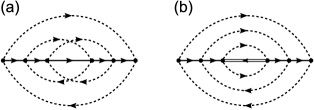
Figure 2: Two examples of diagrams which are not included in our NCA: (a) an example of crossing diagrams and (b) one of the off-shell diagrams which contains intermediate processes at higher energies than the main energy scale, i.e., creation of doublons in the holon propagation. The solid, double-solid, and dashed lines denote the propagators of the holon, the doublon, and the spinon, respectively. Note that the doublon and holon propagators shown here mean a bare propagator, while all lines denote full propagators in Fig. 1.

Consequently, the self-consistent equations of the self-energy of a holon and a doublon are decoupled and given as

$$\Sigma^{\mathrm{h}}(\bm{k},i\nu_{n}) =\left(\frac{W_{\mathrm{h}}}{2\hbar}\right)^{2}\frac{1}{\mathcal{V}}\sum_{\bm{q}}\mathcal{G}^{\mathrm{h}}(\bm{q},i\nu_{n}),$$ (20)

$$\Sigma_{\sigma_{1}\sigma_{2}}^{\mathrm{d}}(\bm{k},i\nu_{n}) =\frac{\left(W_{\mathrm{d}}/2\hbar\right)^{2}}{2(N-1)}\frac{1}{\mathcal{V}}\sum_{\bm{q}}\biggl{[}\sum_{\eta=\sigma_{2}+1}^{\sigma_{1}-1}\mathcal{G}_{\sigma_{1}\eta}^{\mathrm{d}}(\bm{q},i\nu_{n})$$

$$\quad+\sum_{\eta=\sigma_{1}+1}^{N}\mathcal{G}_{\eta\sigma_{2}}^{\mathrm{d}}(\bm{q},i\nu_{n})+\sum_{\eta=1}^{\sigma_{2}-1}\mathcal{G}_{\sigma_{2}\eta}^{\mathrm{d}}(\bm{q},i\nu_{n})$$

$$\quad+N\mathcal{G}_{\sigma_{1}\sigma_{2}}^{\mathrm{d}}(\bm{q},i\nu_{n})\biggr{]},$$ (21)

where $\mathcal{V}$ is the total number of lattice sites. We have also introduced:

$$W_{\mathrm{h}} =\sqrt{4Nzb(\epsilon^{\mathrm{b}})[b(\epsilon^{\mathrm{b}})+1]}J,$$ (22)

$$W_{\mathrm{d}} =\sqrt{8(N-1)zb(\epsilon^{\mathrm{b}})[b(\epsilon^{\mathrm{b}})+1]}J,$$

which correspond to the half bandwidths of the lower and upper Hubbard bands, respectively, as seen below. Because spontaneous breaking of the SU($N$) symmetry is unlikely in the spin-incoherent temperature region, the single-particle property of the doublons is independent of the doublon species:

$$\mathcal{G}^{\mathrm{d}}_{\sigma_{1}\sigma_{2}}(\bm{k},i\nu_{n})\equiv\mathcal{G}^{\mathrm{d}}(\bm{k},i\nu_{n}),$$ (23)

$$\Sigma^{\mathrm{d}}_{\sigma_{1}\sigma_{2}}(\bm{k},i\nu_{n})\equiv\Sigma^{\mathrm{d}}(\bm{k},i\nu_{n}).$$

Then Eq. (21) is simplified more as

$$\Sigma^{\mathrm{d}}(\bm{k},i\nu_{n})=\left(\frac{W_{\mathrm{d}}}{2\hbar}\right)^{2}\frac{1}{\mathcal{V}}\sum_{\bm{q}}\mathcal{G}^{\mathrm{d}}(\bm{q},i\nu_{n}),$$ (24)

which has a form similar to that of Eq. (20). The form of the self-consistent equations (20) and (24) leads to the momentum independence of the self-energies, and thus of the propagators. Using the Dyson equation, the self-consistent equation is analytically solved, and the resulting propagators are

$$\mathcal{G}^{\mathrm{h/d}}(i\nu_{n})=\frac{2}{i\nu_{n}-\frac{\epsilon^{\mathrm{h/d}}}{\hbar}+\sqrt{\left(i\nu_{n}-\frac{\epsilon^{\mathrm{h/d}}}{\hbar}\right)^{2}-\left(\frac{W_{\mathrm{h/d}}}{\hbar}\right)^{2}}}.$$ (25)

Finally, the spectral functions are obtained  via analytic continuation and are:

$$\mathcal{A}^{\mathrm{h/d}}(\omega)=\frac{W_{\mathrm{h/d}}}{4\hbar}\sqrt{1-\left(\frac{\hbar\omega-\epsilon^{\mathrm{h/d}}}{W_{\mathrm{h/d}}}\right)^{2}}.$$ (26)

The spectral function shows the same semicircular behavior as for a single hole in a half-filled $t$-$J$ model discussed in Ref. Kane et al. (1989). Note that in that case the slave bosons would be condensed as a consequence of the long-range antiferromagnetic order. In addition, this result is similar to that of the retraceable path approximation Brinkman and Rice (1970).

The bandwidth (22) as a function of temperature and chemical potential is shown in Fig. 3. $W_{\mathrm{h}}/W_{\mathrm{d}}$ depends only on $N$: $W_{\mathrm{d}}/W_{\mathrm{h}}=\sqrt{2(N-1)/N}$, which monotonically increases and asymptotically reaches $\sqrt{2}$ as $N$ goes up. $W_{\mathrm{d}}$ is larger than $W_{\mathrm{h}}$ for $N>2$. As in Ref. Tokuno et al. (2012), in the SU($2$) case, the shape of the two bands is the same. Figure 3 shows that the temperature dependence is different depending on whether or not $N=2$. While the bandwidth for $N>2$ monotonically increases with temperature, it decreases for $N=2$ and $\mu/U>0$.

Figure 3: (Color online) The holon bandwidth $W_{\mathrm{h}}/\sqrt{4z}J$ for different chemical potentials as a function of temperature and chemical potential: (a) for $N=2$, (b) for $N=6$, and (c) for $N=10$, respectively. The lines from upper to lower denote $\mu/U=0.5$, $0.3$, $0.1$, $0.0$, and $-0.1$, respectively.

Let us look at the single-particle properties of the original fermions. Using the slave-particle representation (6), the Matsubara Green function of the original fermion is expressed as

$$\mathcal{G}_{\sigma,\sigma^{\prime}}(\bm{r}_{j,j^{\prime}},\tau) =-\langle{T_{\tau}h^{\dagger}_{j}(\tau)h_{j}(0)}\rangle\langle{T_{\tau}b_{j,\sigma}(\tau)b_{j^{\prime},\sigma^{\prime}}^{\dagger}(0)}\rangle$$

$$\quad-\sum_{\eta=1}^{\sigma-1}\sum_{\eta^{\prime}=1}^{\sigma^{\prime}-1}\langle{T_{\tau}d_{j,\sigma\eta}(\tau)d^{\dagger}_{j^{\prime},\sigma^{\prime}\eta^{\prime}}(0)}\rangle$$

$$\quad\times\langle{T_{\tau}b_{j,\eta}^{\dagger}(\tau)b_{j^{\prime},\eta^{\prime}}(0)}\rangle$$

$$\quad-\sum_{\eta=\sigma+1}^{N}\sum_{\eta^{\prime}=\sigma^{\prime}+1}^{N}\langle{T_{\tau}d_{j,\eta\sigma}(\tau)d_{j^{\prime},\eta^{\prime}\sigma^{\prime}}^{\dagger}(0)}\rangle$$

$$\quad\times\langle{T_{\tau}b_{j,\eta}^{\dagger}(\tau)b_{j^{\prime},\eta^{\prime}}(0)}\rangle$$

$$\quad+\sum_{\eta=1}^{\sigma-1}\sum_{\eta^{\prime}=\sigma^{\prime}+1}^{N}\langle{T_{\tau}d_{j,\sigma\eta}(\tau)d_{j^{\prime},\eta^{\prime}\sigma}^{\dagger}(0)}\rangle$$

$$\quad\times\langle{T_{\tau}b_{j,\eta}^{\dagger}(\tau)b_{j^{\prime},\eta^{\prime}}(0)}\rangle$$

$$\quad+\sum_{\eta=\sigma+1}^{N}\sum_{\eta^{\prime}=1}^{\sigma^{\prime}-1}\langle{T_{\tau}d_{j,\eta\sigma}(\tau)d_{j^{\prime},\sigma^{\prime}\eta^{\prime}}^{\dagger}(0)}\rangle$$

$$\quad\times\langle{T_{\tau}b_{j,\eta}^{\dagger}(\tau)b_{j^{\prime},\eta^{\prime}}(0)}\rangle,$$ (27)

where $\bm{r}_{j,j^{\prime}}=\bm{r}_{j}-\bm{r}_{j^{\prime}}$, and $T_{\tau}$ denotes the imaginary time order. By applying the mean-field assumption (19) and replacing the atomic propagator in terms of the spinon, the propagator of the original fermion, $\mathcal{G}_{\sigma,\sigma^{\prime}}(\bm{r}_{j,j^{\prime}},\tau)$, is found to be nonzero only for $\sigma=\sigma^{\prime}$ and $\bm{r}_{j}=\bm{r}_{j^{\prime}}$. We thus take $\mathcal{G}_{\sigma,\sigma^{\prime}}(\bm{r}_{j,j^{\prime}},\tau)=\delta_{j,j^{\prime}}\delta_{\sigma,\sigma^{\prime}}\mathcal{G}_{\sigma}(\tau)$. In addition, the assumption of SU($N$) symmetry (23) simplifies more the form of the original fermion propagator. The Fourier transform of the propagator is thus written as

$$\mathcal{G}_{\sigma}(i\nu_{n}) =\frac{1}{\hbar\beta}\sum_{\omega_{l}}\bar{\mathcal{G}}^{\mathrm{b}}_{\mathrm{at}}(i\omega_{l})\biggl{[}\mathcal{G}^{\mathrm{h}}(i\omega_{l}-i\nu_{n})$$

$$\quad-(N-1)\mathcal{G}^{\mathrm{d}}(i\omega_{l}+i\nu_{n})\biggr{]},$$ (28)

and by analytic continuation and Lehmann representation, one can obtain the spectral function as

$$\mathcal{A}_{\sigma}(\bm{k},\omega) =\biggl{[}f(\epsilon^{\mathrm{b}}-\hbar\omega)+b(\epsilon^{\mathrm{b}})\biggr{]}\mathcal{A}_{\mathrm{h}}(\epsilon^{\mathrm{b}}/\hbar-\omega)$$

$$\quad+\biggl{[}f(\epsilon^{\mathrm{b}}+\hbar\omega)+b(\epsilon^{\mathrm{b}})\biggr{]}(N-1)\mathcal{A}_{\mathrm{d}}(\epsilon^{\mathrm{b}}/\hbar+\omega).$$ (29)

The spectral functions for $N=2$, $6$, and $10$ are, respectively, shown in Figs. 6, 6, and 6.

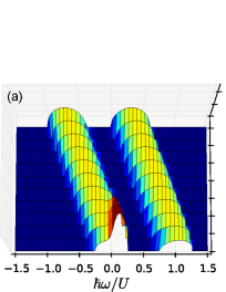
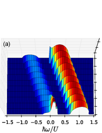
Figure 4: (Color online) The spectral functions of the fermionic atoms for $N=2$ as a function of the chemical potential for different temperatures: (a) $k_{B}T<J$ ($k_{B}T/U=0.025$, $J/U=0.05$), (b) $k_{B}T=J$ ($k_{B}T/U=J/U=0.05$), and (c) $k_{B}T>J$ ($k_{B}T/U=0.075$, $J/U=0.05$). The chemical potential runs from $\mu/U=0$ to $0.7$.

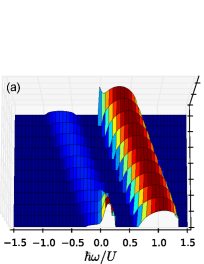
Figure 5: (Color online) The spectral functions of the fermionic atoms for $N=6$ as a function of the chemical potential for different temperatures: (a) $k_{B}T<J$ ($k_{B}T/U=0.025$, $J/U=0.05$), (b) $k_{B}T=J$ ($k_{B}T/U=J/U=0.05$), and (c) $k_{B}T>J$ ($k_{B}T/U=0.075$, $J/U=0.05$). The chemical potential runs from $\mu/U=0$ to $0.7$.

Figure 6: (Color online) The spectral functions of the fermionic atoms for $N=10$ as a function of the chemical potential for different temperatures: (a) $k_{B}T<J$ ($k_{B}T/U=0.025$, $J/U=0.05$), (b) $k_{B}T=J$ ($k_{B}T/U=J/U=0.05$), and (c) $k_{B}T>J$ ($k_{B}T/U=0.075$, $J/U=0.05$). The chemical potential runs from $\mu/U=0$ to $0.7$.

This analytic form implies, as mentioned above, that the holon and doublon spectra form the lower and upper Hubbard bands, respectively. Since the centers of the lower and upper bands are located, respectively, at $\omega=(\epsilon^{\mathrm{d}}-\epsilon^{\mathrm{b}})/\hbar=(U-\mu)/\hbar$ and $-(\epsilon^{\mathrm{h}}-\epsilon^{\mathrm{b}})/\hbar=\mu/\hbar$, the band gap is $U-(W_{\mathrm{h}}+W_{\mathrm{d}})$. For $N>2$, the upper and lower Hubbard bands are always asymmetric because of the absence of particle-hole symmetry. In addition, the weight of the doublon band is larger than that of the holon, because the possible number of doublon states increases with the species of the doublons.

IV Doublon production rate

Using the obtained spectral functions (26), we calculate the DPR spectrum of the optical lattice modulation. In the spectroscopy, the amplitude of an optical lattice in which the atom cloud is confined is modulated, and the created double occupancy is measured as shown in Fig. 7.

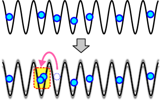
Figure 7: (Color online) A sketch of optical lattice modulation and double occupancy. Due to the modulation perturbation, the system is excited, and doubly occupied sites are created. In experiments, the number of formed atom pairs is measured as a function of the modulation time duration, and the production rate is estimated.

As shown in the Appendix, the DPR per site can be obtained from a second-order calculation  as

$$P_{D}(\omega)=-\frac{(\delta{F})^{2}}{2\hbar\mathcal{V}U}\omega\mathrm{Im}\chi_{\mathrm{K}}^{\mathrm{R}}(\omega),$$ (30)

where $\chi_{\mathrm{K}}(\omega)$ is the Fourier transform of the retarded correlation function of the kinetic energy $\chi_{\mathrm{K}}^{\mathrm{R}}(t)=-i\theta(t)\langle{[T_{t}H_{\mathrm{K}}(t),H_{\mathrm{K}}(0)]}\rangle$, and $\delta{F}$ is the modulation parameter in the lattice model, given by $\delta{F}=[dJ/dV-dU/dV]\delta{V}$, where $\delta{V}$ is the amplitude of the optical lattice modulation.

In order to derive the DPR spectrum formula (30), the system is assumed to be homogeneous, so the trap is not included in the Hamiltonian. It is possible to extend this formulation to an inhomogeneous case Tokuno and Giamarchi (2012). Then the corresponding response function is replaced by

$$(\delta{F})^{2}\chi^{\mathrm{R}}_{\mathrm{K}}(\omega)\rightarrow-i\int_{0}^{\infty}\!\!dt\,\langle{[S(t),S(0)]}\rangle.$$ (31)

The operator $S$ is defined as $S=(\delta{F})H_{\mathrm{K}}-(\delta{U})H_{\mathrm{p}}$ where $\delta{U}=(dU/dV)\delta{V}$ and $H_{\mathrm{p}}$ is the trap potential term of the Hamiltonian. The retarded correlation function is computed using the Hamiltonian $H+H_{\mathrm{p}}$. The above formula can be used directly in situations for which a direct computation of the correlation function in the presence of the trap potential can be implemented by use of numerics such as Monte Carlo simulations and density-matrix renormalization group approaches. However, in general it is not easy to directly deal with the effect of inhomogeneity, and thus we use the LDA to obtain a tractable approximation of (31). In the LDA framework, formula (31) would be identical to the one for the homogeneous case (30). In what follows, we use Eq. (30) to calculate the DPR spectrum in the same manner as discussed in the previous paper Tokuno et al. (2012) in which the inhomogeneity effect of the trap is taken into account by the LDA, and the obtained result shows good agreement with the experimental data Greif et al. (2011).

The DPR is given by the two-particle correlation function, which includes vertex corrections. Here we are in the strongly interacting regime ($J/U\ll 1$), and we ignore the vertex correction as a simple approximation. 

We now compute the retarded correlation function $\chi_{\mathrm{K}}^{\mathrm{R}}(\omega)$ for fillings of one or less than one particle per site in the spin-incoherent intermediate temperature regime. We start with the corresponding imaginary time correlation function $\chi_{\mathrm{K}}(\tau)=-\langle{T_{\tau}H_{\mathrm{K}}(\tau)H_{\mathrm{K}}(0)}\rangle$. In the same way as in the calculation of the spectral function of the original fermions, the analytic continuation of the time-ordered correlation function in imaginary time leads to the retarded correlation function in real time: $\chi_{\mathrm{K}}^{\mathrm{R}}(\omega)=\tilde{\chi}_{\mathrm{K}}(i\omega_{n}\rightarrow\omega+i0^{+})$, where $\tilde{\chi}_{\mathrm{K}}(i\omega_{n})$ is a Fourier transform of $\chi_{\mathrm{K}}(\tau)$. Contrarily to the case of numerical evaluations of correlation functions in imaginary time, for which there is no straightforward way to perform the analytic continuation, here we use our analytic form to do so. This is definitely one of the advantages of the technique used in the present paper, when computing frequency- or time-dependent correlations.

The result for $N=2$ is in extremely good agreement with the experiment of Ref. Greif et al. (2011), as discussed in Ref. Tokuno et al. (2012). As we detail below, a similar analytic calculation can be also done for the case of $N$-component systems, and this allows for a direct comparison to experiments, via the LDA for a trapped system.

The slave-particle representation is useful to clarify the physical meaning of the correlation function $\chi_{\mathrm{K}}(\tau)$. By applying the spin-incoherent assumption (19), the correlation $\chi_{\mathrm{K}}(\tau)$ can be written, for fillings of one or less than one particle per site, as $\chi_{\mathrm{K}}(\tau)=\chi_{\mathrm{K}}^{\mathrm{h}}(\tau)+\chi_{\mathrm{K}}^{\mathrm{d}}(\tau)+\chi_{\mathrm{K}}^{\mathrm{hd}}(\tau)$, where $\chi_{\mathrm{K}}^{\mathrm{h}}(\tau)$, $\chi_{\mathrm{K}}^{\mathrm{d}}(\tau)$, and $\chi_{\mathrm{K}}^{\mathrm{hd}}(\tau)$ are, respectively, given as

$$\chi_{\mathrm{K}}^{\mathrm{h}}(\tau) =NJ^{2}\sum_{\langle{i,j}\rangle}\mathcal{\bar{G}}^{\mathrm{b}}_{\mathrm{at}}(\tau)\mathcal{\bar{G}}^{\mathrm{b}}_{\mathrm{at}}(-\tau)\langle{T_{\tau}h_{i}(\tau)h^{\dagger}_{j}(\tau)h_{j}(0)h_{i}^{\dagger}(0)}\rangle,$$ (32)

$$\chi_{\mathrm{K}}^{\mathrm{d}}(\tau) =J^{2}\sum_{\sigma_{1},\sigma_{2},\sigma_{3},\sigma_{4}}\sum_{\langle{i,j}\rangle}\mathcal{\bar{G}}^{\mathrm{b}}_{\mathrm{at}}(\tau)\mathcal{\bar{G}}^{\mathrm{b}}_{\mathrm{at}}(-\tau)$$

$$\quad\times\langle T_{\tau}D_{i,\sigma_{1}\sigma_{2}}^{\dagger}(\tau)D_{j,\sigma_{1}\sigma_{3}}(\tau)D_{j,\sigma_{4}\sigma_{3}}^{\dagger}(0)D_{i,\sigma_{4}\sigma_{3}}(0)\rangle,$$ (33)

$$\chi_{\mathrm{K}}^{\mathrm{hd}}(\tau) =J^{2}\sum_{\sigma_{1},\sigma_{2}}\sum_{\langle{i,j}\rangle}\biggl{[}[\mathcal{\bar{G}}^{\mathrm{b}}_{\mathrm{at}}(\tau)]^{2}$$

$$\quad\times\langle{T_{\tau}h^{\dagger}_{j}(\tau)D_{i,\sigma_{1}\sigma_{2}}^{\dagger}(\tau)h_{j}(0)D_{i,\sigma_{1}\sigma_{2}}(0)}\rangle$$

$$\quad+(\tau\rightarrow-\tau)\biggr{]}.$$ (34)

They are diagrammatically illustrated in Fig. 8.

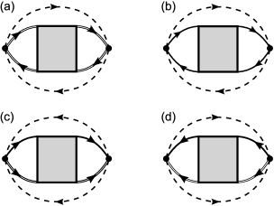
Figure 8: Diagrams corresponding to the kinetic-energy correlation functions: (a) $\chi_{\mathrm{K}}^{\mathrm{h}}(\tau)$, (b) $\chi_{\mathrm{K}}^{\mathrm{d}}(\tau)$, and (c) $\chi_{\mathrm{K}}^{\mathrm{hd}}(\tau)$. The solid, double-solid, and dashed lines, respectively, denote the propagators of the doublon, the holon, and the spinon. The shaded rectangle includes a vertex correction which is not considered in this paper.

In order to simplify the form of the equations the secondary doublon operator $D_{j,\sigma_{1}\sigma_{2}}$, which annihilates the doublon consisting of a $\sigma_{1}$- and a $\sigma_{2}$-component atom at site $j$, has been introduced:

$$D_{j,\sigma_{1}\sigma_{2}}=\left\{\begin{aligned} &d_{j,\sigma_{1}\sigma_{2}}&(\sigma_{1}>\sigma_{2})\\ &0&(\sigma_{1}=\sigma_{2})\\ &-d_{j,\sigma_{2}\sigma_{1}}&(\sigma_{1}<\sigma_{2})\end{aligned}\right..$$ (35)

The correlation function $\chi_{\mathrm{K}}(\tau)$ can be intuitively interpreted as follows: At initial time, a pair consisting of a doublon and a holon is produced by $H_{\mathrm{K}}(0)$, and they move in the system. Then the motion of the created doublon and holon scrambles up the spin configuration of the initial state. For the correlation function to be finite in the spin-incoherent case, the spin configuration of the final state must be the same as the initial one. The most relevant motion would thus be a retraceable path as proposed by Brinkman and Rice Brinkman and Rice (1970). Eventually, the doublon and holon go back to the original point of the production, and the final state created by acting $H_{\mathrm{K}}(\tau)$ reproduces the initial state.

As illustrated in Fig. 9, depending on the spin configuration of the atoms in the initial state, the terms in the correlation function, Eqs. (32)–(34), contribute as follows: $\chi_{\mathrm{K}}^{\mathrm{h}}(\tau)$ for nearest-neighboring pairs of singly occupied and empty sites, $\chi_{\mathrm{K}}^{\mathrm{d}}(\tau)$ for nearest-neighboring pairs of doubly occupied and singly occupied sites, and $\chi_{\mathrm{K}}^{\mathrm{hd}}(\tau)$ for nearest-neighboring pairs of singly occupied sites and pairs of doubly occupied and empty site. From this interpretation, $\chi_{\mathrm{K}}^{\mathrm{h}}(\tau)$ and $\chi_{\mathrm{K}}^{\mathrm{d}}(\tau)$ are expected to be suppressed when the system is at a filling of one particle per site. Thus only $\chi_{\mathrm{K}}^{\mathrm{hd}}(\tau)$ leads to important contributions to the DPR spectrum. In contrast, in going away from the filling of one particle per site, the contributions of $\chi_{\mathrm{K}}^{\mathrm{h}}(\tau)$ and $\chi_{\mathrm{K}}^{\mathrm{d}}(\tau)$ appear.

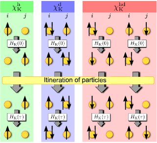
Figure 9: (Color online) A sketch of the contributions to the kinetic-energy correlation function. There are four possible nearest-neighboring pairs in an equilibrium state: (a) singly occupied and empty site, (b) doubly and singly occupied site, (c) singly occupied sites and (d) doubly occupied and empty site. Based on these configurations of the pair of nearest-neighboring sites, we can categorize the three types of contributions, $\chi_{\mathrm{K}}^{\mathrm{h}}(\tau)$ for pair (a) in the left panel, $\chi_{\mathrm{K}}^{\mathrm{d}}(\tau)$ for pair (b) in the middle panel, and $\chi_{\mathrm{K}}^{\mathrm{hd}}(\tau)$ for pairs (c) and (d) in the right panel. The $N=2$ case is taken here for the sake of simplicity, but it can easily be extended to general $N$ cases.

If one neglects vertex corrections, the two-particle correlation functions of Eqs. (32)–(34) are contracted by Wick’s expansion. As a result, the correlation functions are analytically given as

$$\chi_{\mathrm{K}}^{\mathrm{h}}(\tau) =\mathcal{V}NzJ^{2}\mathcal{G}^{\mathrm{b}}(\tau)\mathcal{G}^{\mathrm{b}}(-\tau)\mathcal{G}^{\mathrm{h}}(\tau)\mathcal{G}^{\mathrm{h}}(-\tau),$$ (36)

$$\chi_{\mathrm{K}}^{\mathrm{h}}(\tau) =\mathcal{V}\frac{N(N^{3}-4N+3)}{3}zJ^{2}$$

$$\quad\times\mathcal{G}^{\mathrm{b}}(\tau)\mathcal{G}^{\mathrm{b}}(-\tau)\mathcal{G}^{\mathrm{d}}(\tau)\mathcal{G}^{\mathrm{d}}(-\tau),$$ (37)

$$\chi_{\mathrm{K}}^{\mathrm{hd}}(\tau) =-\mathcal{V}N(N-1)zJ^{2}\biggl{[}\left[\mathcal{G}^{\mathrm{h}}(-\tau)\right]^{2}\mathcal{G}^{\mathrm{h}}(\tau)\mathcal{G}^{\mathrm{d}}(\tau)$$

$$\quad+\left[\mathcal{G}^{\mathrm{h}}(\tau)\right]^{2}\mathcal{G}^{\mathrm{h}}(-\tau)\mathcal{G}^{\mathrm{d}}(-\tau)\biggr{]}.$$ (38)

By moving from the imaginary-time domain to the real-time one by analytic continuation, and by taking the imaginary part of the correlation functions, the analytic form of the DPR per site at a filling of one or less than one particle per site is finally obtained as

$$P_{\mathrm{D}}(\omega) =\frac{(\delta{F})^{2}\omega}{\hbar U}\int\!\!\frac{d\nu}{2\pi}\ \biggl{[}\biggl{(}f(\hbar\nu-\hbar\omega)-f(\hbar\nu)\biggr{)}$$

$$\quad\times\biggl{\{}\frac{W_{\mathrm{h}}^{2}}{8}\mathcal{A}^{\mathrm{h}}(\nu)\mathcal{A}^{\mathrm{h}}(\nu-\omega)+\frac{N(N^{2}+N-3)}{6}\frac{W_{\mathrm{d}}^{2}}{8}$$

$$\quad\times\mathcal{A}^{\mathrm{d}}(\nu)\mathcal{A}^{\mathrm{d}}(\nu-\omega)\biggr{\}}$$

$$\quad+\frac{N(N-1)zJ^{2}\left(1+2b(\epsilon^{\mathrm{b}})\right)}{2}\biggl{(}f(\hbar\nu)+b(2\epsilon^{\mathrm{b}})\biggr{)}$$

$$\quad\times\biggl{(}f(2\epsilon^{\mathrm{b}}-\hbar\nu)-f(2\epsilon^{\mathrm{b}}-\hbar\nu+\hbar\omega)\biggr{)}$$

$$\quad\times\mathcal{A}^{\mathrm{h}}(\nu)\mathcal{A}^{\mathrm{d}}(2\epsilon^{\mathrm{b}}/\hbar-\nu+\omega)$$

$$\quad+\frac{N(N-1)zJ^{2}\left(1+2b(\epsilon^{\mathrm{b}})\right)}{2}\biggl{(}f(\hbar\nu)+b(2\epsilon^{\mathrm{b}})\biggr{)}$$

$$\quad\times\biggl{(}f(2\epsilon^{\mathrm{b}}-\hbar\nu-\hbar\omega)-f(2\epsilon^{\mathrm{b}}-\hbar\nu)\biggr{)}$$

$$\quad\times\mathcal{A}^{\mathrm{h}}(\nu)\mathcal{A}^{\mathrm{d}}(2\epsilon^{\mathrm{b}}/\hbar-\nu-\omega)\biggr{]}.$$ (39)

The DPR spectra for different $N$s and chemical potentials are shown in Figs. 12–12, where the small hopping is fixed to be $J/U=0.05$. To illustrate the temperature dependence, the spectra for $k_{B}T/U=0.025$ ($<J/U$), $0.05$ ($=J/U$), and $0.075$ ($>J/U$) are given.

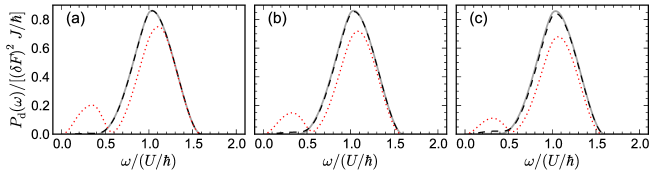
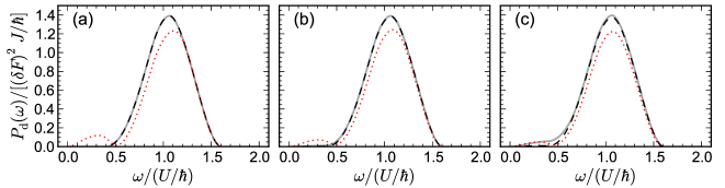
Figure 10: (Color online) The DPR spectra per site, $P_{\mathrm{D}}(\omega)/[(\delta{F})^{2}J/\hbar]$, as a function of modulation frequency for $N=2$ in a cubic lattice ($z=6$): (a) $k_{B}T/U=0.025$ ($k_{B}T<J$), (b) $k_{B}T/U=0.05$ ($k_{B}T=J$), and (c) $k_{B}T/U=0.075$ ($k_{B}T>J$). The hopping parameter is taken to be $J/U=0.05$. The solid, dashed, and dotted lines denote $\mu/U=0.5$, $0.3$, and $0.1$, respectively.

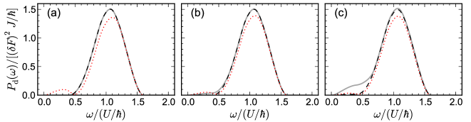
Figure 11: (Color online) The DPR spectra per site, $P_{\mathrm{D}}(\omega)/[(\delta{F})^{2}J/\hbar]$, as a function of modulation frequency for $N=6$ in a cubic lattice ($z=6$): (a) $k_{B}T/U=0.025$ ($k_{B}T<J$), (b) $k_{B}T/U=0.05$ ($k_{B}T=J$), and (c) $k_{B}T/U=0.075$ ($k_{B}T>J$). The hopping parameter is taken to be $J/U=0.05$. The solid, dashed, and dotted lines denote $\mu/U=0.5$, $0.3$, and $0.1$, respectively.

Figure 12: (Color online) The DPR spectra per site, $P_{\mathrm{D}}(\omega)/[(\delta{F})^{2}J/\hbar]$, as a function of modulation frequency for $N=10$ in a cubic lattice ($z=6$): (a) $k_{B}T/U=0.025$ ($k_{B}T<J$), (b) $k_{B}T/U=0.05$ ($k_{B}T=J$), and (c) $k_{B}T/U=0.075$ ($k_{B}T>J$). The hopping parameter is taken to be $J/U=0.05$. The solid, dashed, and dotted lines denote $\mu/U=0.5$, $0.3$, and $0.1$, respectively.

As expected, the dominant peak is found to appear around $\omega=U/\hbar$ for every $\mu/U$ and $N$, and the peak becomes sharper as $\mu/U$ gets closer to $1/2$, and temperature is lowered. Away from filling unity, another small peak in the lower frequency regime appears. It occurs because $\chi_{\mathrm{K}}^{\mathrm{h}}$ becomes relevant due to the hole doping. The spectral weight of this small peak away from filling unity, e.g., at $\mu/U=0.1$, tends to be suppressed for any $N$ as temperature increases. As shown in Fig. 12 and 12, the weight of the peak around $\omega=U/\hbar$ for $N>2$ increases with $N$. This is due to the enhancement caused by the larger spectral weight shown in Figs. 6–6 as $N$ increases. For such $N$s, the spectral weight in the low-frequency regime away from $\mu/U=0.5$, which comes from $\chi_{\mathrm{K}}^{\mathrm{h}}$, is suppressed, in contrast to what happens for the $N=2$ case. However, interestingly, the spectral weight in the low-frequency regime for $N=6$ and $10$ also increases with temperature, while this strong tendency is not seen in the case of $N=2$. This is due to the finite contribution of $\chi_{\mathrm{K}}^{\mathrm{d}}$ because the doublon band enhanced by the larger $N$ reaches $\omega=0$ in such a parameter regime. This is shown in Figs. 6 and 6.

In addition to the plots of Figs. 12–12, we also directly fit our results to the experiment Taie et al. (2012). In such experiments, done with ¹⁷³Yb atoms, the system is expected to be dominated by the MI, and thus our calculation scheme at a filling of one or less than one particle per site would be applicable, using an LDA calculation to take the trap into account. The results, using our theoretical analysis, when taking the parameters corresponding to the experiment are shown in Fig. 13. The experimental parameters, namely, the hopping energy $J/U$, the trap frequency, and the modulation amplitude $\delta{F}$, are taken as follows: (a) $J/U=0.0089$, $2\pi\times(172,139,64)$ [Hz], and $\delta{F}=0.085$, (b) $J/U=0.016$, $2\pi\times(175,141,69)$ [Hz], and $\delta{F}=0.09$, (c) $J/U=0.030$, $2\pi\times(181,146,78)$ [Hz], and $\delta{F}=0.10$, (d) $J/U=0.061$, $2\pi\times(187,151,86)$ [Hz], and $\delta{F}=0.115$, and (e) $J/U=0.091$, $2\pi\times(193,155,86)$ [Hz], and $\delta{F}=0.125$, respectively. The number of atoms in the trap is commonly assumed to be $1.87\times 10^{4}$. The following temperatures are determined by the least-square fits to the experimental data: (a) $k_{B}T/U=0.0719$, (b) $k_{B}T/U=0.0577$, (c) $k_{B}T/U=0.0909$, (d) $k_{B}T/U=0.0963$, and (e) $k_{B}T/U=0.179$. Figure 13 shows good agreement with the experimental result, which supports the validity of our theory.

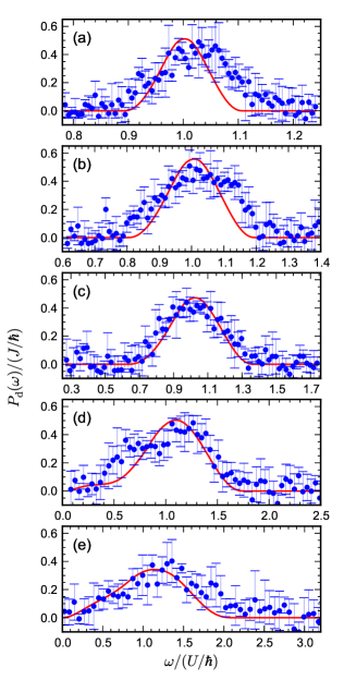
Figure 13: (Color online) The dimensionless DPR spectra $P_{\mathrm{d}}(\omega)$ scaled by $J/\hbar$ as a function of modulation frequency $\hbar\omega/U$ for an $N=6$ trapped system with different parameters: (a) $J/U=0.0089$, (b) $J/U=0.016$, (c) $J/U=0.030$, (d) $J/U=0.061$, and (e) $J/U=0.091$. In all cases, $1.87\times 10^{4}$ trapped atoms and a modulation amplitude $\delta{F}=0.08$ are taken. The solid line and points with an error bar, respectively, denote the theoretical result and the ¹⁷³Yb experiments Taie et al. (2012). The temperatures are determined by the least-square fit to the experiment, and the values are (a) $k_{B}T/U=0.0719$, (b) $k_{B}T/U=0.0577$, (c) $k_{B}T/U=0.0909$, (d) $k_{B}T/U=0.0963$, and (e) $k_{B}T/U=0.179$.

V Summary

We have computed doublon and holon excitations of strongly interacting $N$-component fermions in optical lattices in the spin-incoherent regime. This corresponds to a temperature region between the superexchange coupling and the interaction. As an effective Hamiltonian to extract the physics at an energy scale of order $\sim U$, the symmetric SU($N$) Hubbard model has been studied, which means that the Hubbard interaction is independent of the internal degree of freedom of the fermions. The theory presented in Ref. Tokuno et al. (2012), which reproduces well the experiment with ⁴⁰K atoms Greif et al. (2011), has been extended to an $N$-component fermion case, and the analytic form of the single-particle spectral functions for fillings of one or less than one particle per site has been obtained. Our approach is based on the slave-particle representation in which the original fermion operators are represented by a fermionic holon, $N$ species of bosonic spinons, and $N(N-1)/2$ species of fermionic doublons. We have employed a combination of mean-field theory, a diagrammatic approach, and the NCA to take into account the finite particle hopping $J$, and we have captured the physics of the hole-doped systems for large interaction $J\ll U$.

As an application to the calculation of the experimental observables, the DPR induced by dynamical periodic modulation of optical lattices as a function of modulation frequency has been also computed, both for the homogeneous system and for the trapped system, in an LDA. As shown in the Appendix, the DPR spectrum as a second-order response to the optical lattice modulation is directly related to the retarded kinetic-energy correlation function. We have discussed the DPR spectrum without vertex corrections, and we have presented the analytic form constructed by the obtained spectral functions of the doublon and the holon.

From the obtained analytic form in the case of homogeneous systems, we have obtained the DPR spectra as a function of temperature, chemical potential, and component number $N$, and we have compared the different behaviors for the different $N$s. While the large peak structure around the interaction $U$ exists regardless of the value of $N$, some differences have been observed in the regime of low modulation frequency. In the comparison, we have focused on two different effects leading to an enhancement of the spectral weight in the low-frequency regime. The first one is a doping effect: in going away from half-filling, the low-frequency spectrum appears as a consequence of the system becoming metallic. This effect has been found to be suppressed as $N$ increase. The second effect is the temperature: the spectral weight in the low-frequency side tends to increase with temperature. However, unlike the first effect, we find that the spectral weight is enhanced as $N$ goes up. Therefore the properties of the spectra for different $N$s will be most markedly different for the low-energy part of the spectrum.

The theory presented in this paper has several advantages: First, the finite-temperature dynamics can be dealt with analytically. For such dynamical correlations, numerical approaches cannot be straightforwardly applied because of the difficulty of numerical implementation of the analytic continuation; second, our theoretical technique allows for the control of the chemical potential, in principle. Note however that our approximations are expected to work well at a filling close to the MI state. This means that inhomogeneous systems in the presence of a trap potential can be also discussed by using an LDA. Indeed, in Ref. Tokuno et al. (2012), this approach has been applied to the SU($2$) symmetric Hubbard model with a harmonic trap potential, and quantitatively precise agreement with the experiment Greif et al. (2011) has been obtained.

Using the extension of this approach to trapped systems we have compared our results for the DPR spectra shown in Fig. 13, for which the presence of the trap potential is taken into account by LDA, with ¹⁷³Yb experiments. The temperature has been determined by the best fit to the experimental data Taie et al. (2012), and the obtained results for the DPR peak are in good agreement with the experiment.

In recent years, the symmetric SU($N$) systems have been being realized in experiments with alkaline-earth-metal(-like) ⁸⁷Sr Ye et al. (2008); DeSalvo et al. (2010); Tey et al. (2010) in addition to ¹⁷³Yb atoms. Current fermionic atom systems in such experiments are still at high temperature. Therefore our theory is expected to work very effectively to compare up-coming lattice modulation experiments in such a temperature regime.

Finally, we would like to mention some prospects of our study. The first is to apply this technique to the calculation of thermodynamic functions such as entropy. It is hard to measure temperature directly in experiments, and the measurement of entropy is used instead. Thus by computing the entropy within our theoretical framework, we can make a more straightforward comparison with the experiment. The second is to extend the theory to general $N$-component mixtures away from the SU($N$) symmetry limit. Although the SU($N$) symmetry has been assumed throughout this paper, the slave-particle representation and the NCA calculation would be still applicable away from the SU($N$) symmetric point. However, the self-consistent equations for the self-energies [Eqs. (20) and (21)] remain complicated, and the issue would be how to solve the self-consistent equations. Another prospect is to develop this technique to capture the low-temperature physics. The difficulty of the application of the present technique to spin-coherent systems is that we have here assumed fully incoherent spins. Namely, the spinon propagators are replaced by the atomic propagators, which means that even nearest-neighbor spin correlations are ignored. Thus the key to improve the technique for lower temperature would be to modify the spin-incoherence assumption (15) . Such an improved technique would allow for the crosscheck of the theoretical predictions Bon ; Mes .

Appendix A Formulation of DPR spectra

The derivation of the DPR formula is briefly reviewed. For simplicity, we only consider the homogeneous case, but the more general case including an inhomogeneous potential such as a trap can be discussed. Such a general argument can be found in Ref. Tokuno and Giamarchi (2012). We start with a generic Hamiltonian of interacting atoms in optical lattice potentials defined in $D$-dimensional continuum space, which is written as follows:

$$H=H_{0}+\int\!\!d\bm{r}V_{\rm op}(\bm{r})\rho(\bm{r}),$$ (40)

where $V_{\rm op}(\bm{r})=\sum_{\mu=1}^{D}V_{0}\cos^{2}(kx_{\mu})$ is the optical lattice potential, and $H_{0}$ is an unperturbed Hamiltonian of interacting atoms in free space.

For a deep optical lattice potential ($V_{0}\gg\mu$), the Hamiltonian $H$ is well described by the Hubbard model. Then the parameters, the hopping $J$ and on-site interaction $U$, are given as a function of lattice depth $V_{0}$. For example, if the Wannier function is assumed to be approximated as a Gaussian wave function, the hopping $J$ and on-site interaction $U$ are estimated Bloch et al. (2008) as

$$J \approx\frac{4}{\sqrt{\pi}}E_{\mathrm{R}}\left(\frac{V_{0}}{E_{\mathrm{R}}}\right)^{3/4}\exp\left[-2\sqrt{\frac{V_{0}}{E_{\mathrm{R}}}}\right],$$ (41)

$$U \approx\frac{8}{\pi}ka_{\mathrm{s}}E_{\mathrm{R}}\left(\frac{V_{0}}{E_{\mathrm{R}}}\right)^{3/4},$$ (42)

where $E_{\mathrm{R}}$ and $a_{\mathrm{s}}$ are, respectively, the recoil energy and $s$-wave scattering length of atoms in free space.

We consider an amplitude modulation perturbation of an optical lattice. For deep lattices the modulation effect of the lattice potential can be described by replacing the amplitude of the static lattice potential $V_{\mathrm{op}}$ as $V_{0}\rightarrow V_{0}[1+\delta{V}\cos(\omega t)]$. Then the parameters of the lattice model also follow the replacement, and the modulation parts are derived up to first order in $\delta{V}$:

$$U \rightarrow U[1+\delta{U}\cos(\omega t)],$$ (43)

$$J \rightarrow J[1+\delta{J}\cos(\omega t)],$$ (44)

where $\delta{U}=(\partial{\ln{U}}/\partial{V_{0}})V_{0}$ and $\delta{J}=(\partial{\ln{J}}/\partial{V_{0}})V_{0}$. In the case of a Gaussian Wannier function (41) and (42), $\delta{U}\approx 3/4$ and $\delta{J}\approx 3/4-\sqrt{V_{0}/E_{\mathrm{R}}}$. Thus the time-dependent perturbation by lattice modulation is written as $(\delta{U}H_{\mathrm{U}}+\delta{J}H_{\mathrm{K}})\cos(\omega t)$, where $H_{\mathrm{U}}=U\sum_{j,\sigma_{1}>\sigma_{2}}n_{j,\sigma_{1}}n_{j,\sigma_{2}}$. In addition, by making use of the form of the Hubbard Hamiltonian, the perturbation can be rewritten as $\delta{U}H\cos(\omega t)+\delta{F}H_{\mathrm{K}}\cos(\omega t)$, where $\delta{F}=\delta{J}-\delta{U}$. Thus the considered Hamiltonian with the lattice modulation is written as

$$H(t)=H+\delta{U}H\cos(\omega t)+\delta{F}H_{\mathrm{K}}\cos(\omega t).$$ (45)

Extending the doublon number projector for $N=2$, we can define the total number operator of a doublon by the Hubbard interaction as

$$N_{\rm D}=\frac{1}{U}H_{\mathrm{U}},$$ (46)

where we have defined the total doublon number as a total sum of all species of doublons. This projection operator (46) truncates only the empty and singly occupied state, and thus it could not count the doublon number perfectly for $N>2$ since the projected states include multiparticle occupancies of more than three such as three- and four-fold occupancy and so on. However, because such multiparticle occupations are away from the main energy scale in the case considered here , Eq. (46) would be also identical to the total doublon number in the case of multicomponent fermions. The DPR per site is defined as a time average of time derivative of $N_{\mathrm{D}}$ over a single period of modulation:

$$P_{\mathrm{D}}(\omega)\equiv\frac{1}{2\pi/\omega}\int_{T}^{T+2\pi/\omega}\!\!dt\ \frac{d}{dt}\frac{\langle{N}_{\mathrm{D}}\rangle}{\mathcal{V}},$$ (47)

where $\langle{\cdots}\rangle$ means the thermodynamic average by the Hamiltonian (45), and $\mathcal{V}$ is the total number of lattice sites.

We implement second-order perturbation theory in term of $d\langle{N_{\mathrm{D}}}\rangle/dt$. Then we use the following mathematical trick: Using Eq. (45), we rewrite the total doublon number operator as

$$N_{\mathrm{D}}=\frac{1}{U}\biggl{[}H(t)-H_{\mathrm{K}}-(H+\delta{F}H_{\mathrm{K}})\cos(\omega t)\biggr{]}.$$ (48)

From a straightforward calculation up to second order, the terms apart from $H(t)$ are found to contribute as oscillatory terms, and they cancel due to the single-period time average. Thus $P_{\mathrm{D}}(\omega)$ can be rewritten as

$$P_{\mathrm{D}}(\omega)\equiv\frac{1}{2\pi/\omega}\int_{T}^{T+2\pi/\omega}\!\!dt\ \frac{\langle{\dot{H(t)}}\rangle}{\mathcal{V}},$$ (49)

where we have used the identity $d\langle{H(t)}\rangle/dt=\langle{\dot{H}(t)}\rangle$. This is equivalent to the definition of the energy absorption rate Tokuno and Giamarchi (2011). This equivalence was numerically established for spin-$1/2$ one-dimensional fermions in Ref. Kollath et al. (2006). The second-order response of the energy absorption rate can be calculated by linear response. Therefore one can finally obtain the formula as

$$P_{\rm D}(\omega)=-\frac{(\delta{F})^{2}}{2\hbar\mathcal{V}U}\omega\,\mathrm{Im}\,{\tilde{\chi}^{\mathrm{R}}_{\mathrm{K}}(\omega)},$$ (50)

where $\tilde{\chi}^{\rm R}_{\mathrm{K}}(\omega)$ is a Fourier component of the kinetic-energy-retarded correlation function $\chi^{\mathrm{R}}_{\mathrm{K}}(t)=-i\theta(t)\langle[H_{\mathrm{K}}(t),H_{\mathrm{K}}(0)]\rangle_{0}$ where $\langle{\cdots}\rangle_{0}$ denotes the statistical average by the unperturbed Hamiltonian $H$.

References

- Esslinger (2010) T. Esslinger, Annu. Rev. Condens. Matter Phys. 1, 129 (2010).
- Bloch et al. (2008) I. Bloch, J. Dalibard, and W. Zwerger, Rev. Mod. Phys. 80, 885 (2008).
- Imada et al. (1998) M. Imada, A. Fujimori, and Y. Tokura, Rev. Mod. Phys. 70, 1039 (1998).
- Lee et al. (2006) P. A. Lee, N. Nagaosa, and X.-G. Wen, Rev. Mod. Phys. 78, 17 (2006).
- Taie et al. (2010) S. Taie, Y. Takasu, S. Sugawa, R. Yamazaki, T. Tsujimoto, R. Murakami, and Y. Takahashi, Phys. Rev. Lett. 105, 190401 (2010).
- Fukuhara et al. (2007) T. Fukuhara, Y. Takasu, M. Kumakura, and Y. Takahashi, Phys. Rev. Lett. 98, 030401 (2007).
- Cazalilla et al. (2009) M. A. Cazalilla, A. F. Ho, and M. Ueda, New Journal of Physics 11, 103033 (2009).
- Ye et al. (2008) J. Ye, H. J. Kimble, and H. Katori, Science 320, 1734 (2008).
- Hermele et al. (2009) M. Hermele, V. Gurarie, and A. M. Rey, Phys. Rev. Lett. 103, 135301 (2009).
- Hermele et al. (2011) M. Hermele, V. Gurarie, and A. M. Rey, Phys. Rev. Lett. 107, 059901(E) (2011).
- DeSalvo et al. (2010) B. J. DeSalvo, M. Yan, P. G. Mickelson, Y. N. Martinez de Escobar, and T. C. Killian, Phys. Rev. Lett. 105, 030402 (2010).
- Manmana et al. (2011) S. R. Manmana, K. R. A. Hazzard, G. Chen, A. E. Feiguin, and A. M. Rey, Phys. Rev. A 84, 043601 (2011).
- Honerkamp and Hofstetter (2004) C. Honerkamp and W. Hofstetter, Phys. Rev. Lett. 92, 170403 (2004).
- Gorshkov et al. (2010) A. V. Gorshkov, M. Hermele, V. Gurarie, C. Xu, P. S. Julienne, J. Ye, P. Zoller, E. Demler, M. D. Lukin, and A. M. Rey, Nature Phys. 6, 289 (2010).
- Hazzard et al. (2012) K. R. A. Hazzard, V. Gurarie, M. Hermele, and A. M. Rey, Phys. Rev. A 85, 041604 (2012).
- Nonne et al. (2010) H. Nonne, P. Lecheminant, S. Capponi, G. Roux, and E. Boulat, Phys. Rev. B 81, 020408 (2010).
- Nonne et al. (2011a) H. Nonne, E. Boulat, S. Capponi, and P. Lecheminant, Modern Physics Letters B (MPLB) 25, 955 (2011a).
- Nonne et al. (2011b) H. Nonne, P. Lecheminant, S. Capponi, G. Roux, and E. Boulat, Phys. Rev. B 84, 125123 (2011b).
- Azaria et al. (2009) P. Azaria, S. Capponi, and P. Lecheminant, Phys. Rev. A 80, 041604 (2009).
- Arovas and Auerbach (1988) D. P. Arovas and A. Auerbach, Phys. Rev. B 38, 316 (1988).
- Read and Sachdev (1989) N. Read and S. Sachdev, Phys. Rev. Lett. 62, 1694 (1989).
- Read and Sachdev (1990) N. Read and S. Sachdev, Phys. Rev. B 42, 4568 (1990).
- Harada et al. (2003) K. Harada, N. Kawashima, and M. Troyer, Phys. Rev. Lett. 90, 117203 (2003).
- Kawashima and Tanabe (2007) N. Kawashima and Y. Tanabe, Phys. Rev. Lett. 98, 057202 (2007).
- Ruckenstein and Schmitt-Rink (1988) A. E. Ruckenstein and S. Schmitt-Rink, Phys. Rev. B 38, 7188 (1988).
- Affleck and Marston (1988) I. Affleck and J. B. Marston, Phys. Rev. B 37, 3774 (1988).
- Marston and Affleck (1989) J. B. Marston and I. Affleck, Phys. Rev. B 39, 11538 (1989).
- Lavagna et al. (1987) M. Lavagna, A. J. Millis, and P. A. Lee, Phys. Rev. Lett. 58, 266 (1987).
- Kotliar and Liu (1988) G. Kotliar and J. Liu, Phys. Rev. Lett. 61, 1784 (1988).
- Abrikosov (1965) A. A. Abrikosov, Physics 2, 5 (1965).
- Barnes (1976) S. E. Barnes, Journal of Physics F: Metal Physics 6, 1375 (1976).
- Read and Newns (1983) N. Read and D. M. Newns, Journal of Physics C: Solid State Physics 16, 3273 (1983).
- Coleman (1984) P. Coleman, Phys. Rev. B 29, 3035 (1984).
- Kotliar and Ruckenstein (1986) G. Kotliar and A. E. Ruckenstein, Phys. Rev. Lett. 57, 1362 (1986).
- Li et al. (1989) T. Li, P. Wölfle, and P. J. Hirschfeld, Phys. Rev. B 40, 6817 (1989).
- Lavagna (1990) M. Lavagna, Phys. Rev. B 41, 142 (1990).
- Kane et al. (1989) C. L. Kane, P. A. Lee, and N. Read, Phys. Rev. B 39, 6880 (1989).
- Marsiglio et al. (1991) F. Marsiglio, A. E. Ruckenstein, S. Schmitt-Rink, and C. M. Varma, Phys. Rev. B 43, 10882 (1991).
- Sensarma et al. (2009) R. Sensarma, D. Pekker, M. D. Lukin, and E. Demler, Phys. Rev. Lett. 103, 035303 (2009).
- Huber and Rüegg (2009) S. D. Huber and A. Rüegg, Phys. Rev. Lett. 102, 065301 (2009).
- Tokuno et al. (2012) A. Tokuno, E. Demler, and T. Giamarchi, Phys. Rev. A 85, 053601 (2012).
- Stöferle et al. (2004) T. Stöferle, H. Moritz, C. Schori, M. Köhl, and T. Esslinger, Phys. Rev. Lett. 92, 130403 (2004).
- Iucci et al. (2006) A. Iucci, M. A. Cazalilla, A. F. Ho, and T. Giamarchi, Phys. Rev. A 73, 041608 (2006).
- Reischl et al. (2005) A. Reischl, K. P. Schmidt, and G. S. Uhrig, Phys. Rev. A 72, 063609 (2005).
- Kollath et al. (2006) C. Kollath, A. Iucci, I. P. McCulloch, and T. Giamarchi, Phys. Rev. A 74, 041604 (2006).
- Tokuno and Giamarchi (2011) A. Tokuno and T. Giamarchi, Phys. Rev. Lett. 106, 205301 (2011).
- Tokuno and Giamarchi (2012) A. Tokuno and T. Giamarchi, Phys. Rev. A 85, 061603 (2012).
- Jördens et al. (2008) R. Jördens, N. Strohmaier, K. Günter, H. Moritz, and T. Esslinger, Nature 455, 204 (2008).
- Greif et al. (2011) D. Greif, L. Tarruell, T. Uehlinger, R. Jördens, and T. Esslinger, Phys. Rev. Lett. 106, 145302 (2011).
- Taie et al. (2012) S. Taie, R. Yamazaki, S. Sugawa, and Y. Takahashi, Nature Phys. 8, 825 (2012).
- Kitagawa et al. (2008) M. Kitagawa, K. Enomoto, K. Kasa, Y. Takahashi, R. Ciuryło, P. Naidon, and P. S. Julienne, Phys. Rev. A 77, 012719 (2008).
- Stellmer et al. (2011) S. Stellmer, R. Grimm, and F. Schreck, Phys. Rev. A 84, 043611 (2011).
- Note (1) For example, it is known that for 173Yb atoms, which are spin- fermions, all two-body interactions are the same.
- Note (2) At a filling of one particle per site, the system for would become a Mott insulator. The charge coherence should then be suppressed even if . Thus, the spin-incoherent temperature regime at unity filling is .
- Brinkman and Rice (1970) W. F. Brinkman and T. M. Rice, Phys. Rev. B 2, 1324 (1970).
- Note (3) In the present case, the spectral function is a local quantity. Thus it corresponds to the density of state.
- Note (4) Here the DPR is defined as the number of doubly occupied sites. In Ref. Greif et al. (2011), it is defined as the number of atoms forming doublons.
- Note (5) Vertex corrections are usually needed to preserve symmetries which are broken in mean-field calculations. However, in this case there is no spontaneous symmetry breaking in our mean-field calculation. Thus, the vertex correction would only give a quantitative correction. In the strongly interacting case this correction will be small.
- Tey et al. (2010) M. K. Tey, S. Stellmer, R. Grimm, and F. Schreck, Phys. Rev. A 82, 011608 (2010).
- (60) L. Bonnes, K. R. A. Hazzard, S. R. Manmana, A. M. Rey, and S. Wessel, arXiv:1207.3900.
- (61) L. Messio and F. Mila, arXiv:1207.1320.