Analytical Solution of Cross Polarization Dynamics

Abstract

Cross polarization (CP) dynamics, which was remained unknown for five decades, has been derived analytically in the zero- and double-quantum spaces. The initial polarization in the double-quantum space is a constant of motion under strong pulse condition ($|\omega_{1I}+\omega_{1S}|\gg|d(t)|$), while the Hamiltonian in the zero-quantum space reduces to $d(t)\sigma_{z}^{\Delta}$ under the Hartmann-Hahn match condition ($\omega_{1I}=\omega_{1S}$). The time dependent Hamilontian ($d(t)\sigma_{z}^{\Delta}$) in the zero-quantum space can be expressed by average Hamiltonians. Since$[d(t^{\prime})\sigma_{z}^{\Delta},d(t^{\prime\prime})\sigma_{z}^{\Delta}]=0$, only zero order average Hamiltonian needs to be calculated, leading to an analytical solution of CP dynamics.

I 1. Introduction

Cross polarization (CP), developed by Hartmann and Hahn HartmannHah in 1962 and later modified by Pines et al Pines , is one of the most important techniques in NMR. Mediated by heteronuclear dipolar interaction, polarization is often transferred from abundant I spins to a rare S spin with a polarization enhancement up to $\gamma_{I}/\gamma_{S}$. Because the overall delay time is just only subject to the spin-lattice relaxation time of I spins, considerable NMR time is saved compared with a single pulse experiment.

CP dynamics for a single crystal was first derived by Müller et al Ernst . For a stationary sample, the Hamiltonian is time independent, it can also be solved by diagonalization of the Hamiltonians. Under fast magic angle spinning(MAS) ($\omega_{r}/2\pi\gg|d(t)|$), the Hartman-Hahn match condition shift to $\omega_{1I}-\omega_{1S}=n\omega_{r}$($n=\pm 1,2$) Stejskcal and the effective heteronuclear dipolar interaction becomes time independent Shanmin1 . Consequently the CP dynamics under fast MAS can be derived without many problems Shanmin1 , in particular under Lee-Goldburg (LG) LG condition as demonstrated by Ladizhansky et al LGCP ; Vega . However, under conventional MAS speed, the heteronuclear dipolar interaction becomes time dependent, as many other quantum systems, searching for an analytic solution is usually not conceivable.

So far, CP dynamics under conventional MAS speed is usually calculated with a spin temperature hypothesis Mehring ; Goldman . It inevitably leads to an empirical solution ChemRev . In the zero- and double-quantum spaces Levitt , which commutes with each other, the evolution of density matrix can be done separately in the two spaces, simplifying the calculation considerably. By means of this method, a number of intriguing phenomena in CP has been understood thoroughly. They include CP dynamics of phase-shifted CP under mismatch conditions Levitt ; Shanmin2 , W-MOIST WMOIST , double-quantum matched CP Meier ; Shanmin1 , and adiabatic polarization transfer Adiabatic ; Shanmin1 .

Up to now, CP dynamics under conventional MAS speed and the Hartman-Hahn match condition ($\omega_{1I}=\omega_{1S}$) has remained unknown. In this article we show that this problem can be resolved in the zero- and double-quantum spaces together with average Hamiltionian theory AHT . The experiment and simulated results match well with the theoretical predictions.

II 2. Theory

For a heteronuclear dipolar coupled $IS$ spin pair under cross polarization and magic angle spinning (CPMAS), the Hamiltonian can be described by

$$\mathcal{H}=\omega_{1I}I_{y}+\omega_{1S}S_{y}+2d(t)I_{z}S_{z},$$ (1)

where $\omega_{1I}$ and $\omega_{1S}$ are the strengths of the I and S spin-locking fields, respectively, and

$$\begin{split}d(t)&=d[\sqrt{2}sin(2\beta)cos(\omega_{r}t+\gamma)\\ &-sin^{2}(\beta)cos(2\omega_{r}t+2\gamma)]\end{split}$$ (2)

is a time dependent heteronuclear dipolar coupling constant with two Euler angles in the rotor-fixed frame. In the zero- and double-quantum spaces, the above Hamiltonian can be expressed as Levitt ; Shanmin1 ; Shanmin2 ; WMOIST

$$\mathcal{H}^{\Delta}=d(t)\sigma_{z}^{\Delta}+(\omega_{1I}-\omega_{1S})\sigma_{y}^{\Delta}\ (zero-quantum)$$ (3)

and

$$\mathcal{H}^{\Sigma}=d(t)\sigma_{z}^{\Sigma}+(\omega_{1I}+\omega_{1S})\sigma_{y}^{\Sigma}\ (double-quantum),$$ (4)

where $\sigma_{i}^{\Delta}$ and $\sigma_{i}^{\Sigma}$ are the Pauli matrices. The initial density matrix can be expressed in terms of zero-quantum and double-quantum density matrices

$$\rho(0)=I_{y}=\frac{1}{2}(I_{y}-S_{y})+\frac{1}{2}(I_{y}+S_{y})=\sigma_{y}^{\Delta}+\sigma_{y}^{\Sigma}.$$ (5)

Because $[\sigma_{i}^{\Delta},\sigma_{i}^{\Sigma}]=0(i,j=x,y,z)$ and $[\mathcal{H}^{\Delta},\mathcal{H}^{\Sigma}]=0$, the evolution of density matrix can be calculated in the zero- and double-quantum spaces separately,

$$\begin{split}\rho(t)&=\sigma^{\Delta}(t)+\sigma^{\Sigma}(t)\\ &=e^{-i\int_{0}^{t}\mathcal{H}^{\Delta}(t^{\prime})dt^{\prime}}\sigma_{y}^{\Delta}e^{\int_{0}^{t}\mathcal{H}^{\Delta}(t^{\prime})dt^{\prime}}\\ &+e^{-i\int_{0}^{t}\mathcal{H}^{\Sigma}(t^{\prime})dt^{\prime}}\sigma_{y}^{\Sigma}e^{\int_{0}^{t}\mathcal{H}^{\Sigma}(t^{\prime})dt^{\prime}}.\end{split}$$ (6)

Under strong pulse condition $|\omega_{1I}+\omega_{1S}|\gg|d(t)|$, the density matrix in the double-quantum space is nearly a constant of motion, i.e.

$$\sigma^{\Sigma}(t)\approx\sigma_{y}^{\Sigma}.$$ (7)

Therefore, the calculation of density matrix is largely determined by the evolution in the zero-quantum space. Under Hartmann-Hahn match condition $\omega_{1I}=\omega_{1S}$, the Hamiltonian in the zero-quantum space becomes

$$\mathcal{H}^{\Delta}(t)=d(t)\sigma_{z}^{\Delta},$$ (8)

which is time dependent. For every particular time, it can be represented by a zero-order average Hamiltonian

$$\begin{split}\overline{\mathcal{H}}^{\Delta(0)}&(t)=\frac{\sigma_{z}^{\Delta}}{t}\int_{0}^{t}d(t^{\prime})dt^{\prime}=\overline{d}(t)\sigma_{z}^{\Delta}\\ &=\frac{d}{2t}\{2\sqrt{2}sin(2\beta)[sin(\omega_{r}t+\gamma)-sin(\gamma)]\\ &-sin^{2}(\beta)[sin(2\omega_{r}t+2\gamma)-sin(2\gamma)]\}\sigma_{z}^{\Delta}.\end{split}$$ (9)

Since $[\mathcal{H}^{\Delta}(t^{\prime}),\mathcal{H}^{\Delta}(t^{\prime\prime})]=0$ for any $t^{\prime}$ and $t^{\prime\prime}$, all the higher order Hamiltonians vanish. Consequently, the zero-order average Hamiltonian represents exactly the Hamiltonian of the spin system. It turns out that the average Hamiltonian itself is time dependent, but for any particular time t it can be treated as a time independent Hamiltonian in the evolution of density matrix. Therefore, for a given average Hamiltonian the density matrix in the zero-quantum space can be derived

$$\begin{split}\sigma^{\Delta}(t)&=e^{-i\overline{d}(t)\sigma_{z}^{\Delta}}\sigma_{y}^{\Delta}e^{i\overline{d}(t)\sigma_{z}^{\Delta}}\\ &=cos(\overline{d}(t))\sigma_{y}^{\Delta}-sin(\overline{d}(t))\sigma_{x}^{\Delta}.\end{split}$$ (10)

Base on the Eqs. (6), (7), and (10), the evolution of density matrix becomes

$$\begin{split}\rho(t)&=\sigma^{\Delta}(t)+\sigma^{\Sigma}(t)\\ &=cos(\overline{d}(t))\sigma_{y}^{\Delta}-sin(\overline{d}(t))\sigma_{x}^{\Delta}+\sigma_{y}^{\Sigma},\end{split}$$ (11)

which leads to a CP dynamics

$$\begin{split}CP(t)&=Trace<S_{y}\cdot\rho(t)>\\ &=Trace<(\sigma_{y}^{\Sigma}-\sigma_{y}^{\Delta})\cdot\rho(t)>\\ &=1-cos(\overline{d}(t)).\end{split}$$ (12)

The CP dynamics of powder sample can be derived by integration over the Euler solid angle on the sphere

$$CP(t)=\int_{0}^{\pi}\!\!\!\int_{0}^{2\pi}\!\!\!\{1-cos[\overline{d}(t)]\}sin(\beta)d\beta d\gamma.$$ (13)

Considering the effects of I spin diffusion and spin lattice relaxation in the rotating frame, the CP dynamics becomes

$$\begin{split}M(t)&=M_{0}\cdot\{1-\frac{1}{2}e^{-Rt}\\ &-\frac{1}{2}e^{-R_{1}t}(1-2\cdot CP(t))\}\cdot e^{-\frac{t}{T_{1\rho}}},\end{split}$$ (14)

where $R$ is the spin diffusion rate of I spin, $R_{1}$ is a rate which results in the oscillation damping by the remote I spins, and $T_{1\rho}$ is the spin lattice relaxation in the rotating frame of the I spins.

When $\omega_{r}\rightarrow 0$, the Eq. (14) reduce to:

$$M(t)=M_{0}\cdot\{1-\frac{1}{2}e^{-Rt}-\frac{1}{2}e^{-R_{1}t}cos(dt)\}\cdot e^{-\frac{t}{T_{1\rho}}}$$ (15)

which, except for the T1 effect, is identical to the result by Müller et al Ernst for a stationary sample.

In the above calculation, the offsets, $\Delta\omega_{I}$ and $\Delta\omega_{S}$ for I and S spin, are ignored. Under off-resonance condition, the Hartman-Hahn match condition is determined by effective fields, i.e. $\omega_{1Ie}=\omega_{1Se}$, where

$$\begin{split}&\omega_{1Ie}=\sqrt{\Delta\omega_{I}^{2}+\omega_{1I}^{2}}\qquad and\\ &\omega_{1Se}=\sqrt{\Delta\omega_{S}^{2}+\omega_{1S}^{2}}.\end{split}$$ (16)

Correspondingly, the dipolar interaction is split up into two parts (perpendicular and parallel)

$$\begin{split}d(t)I_{z}S_{z}&=sin(\theta_{I})sin(\theta_{S})d(t)I_{ze}S_{ze}\\ &+cos(\theta_{I})cos(\theta_{S})d(t)I_{ye}S_{ye},\end{split}$$ (17)

where

$$\begin{split}&\theta_{I}=cos^{-1}(\Delta\omega_{I}/\omega_{1Ie})\qquad and\\ &\theta_{S}=cos^{-1}(\Delta\omega_{S}/\omega_{1Se}).\end{split}$$ (18)

In Eq. (17), the perpendicular term is responsible for polarization transfer while the parallel term is a small perturbation which can be ignored here. In the perpendicular term, the dipolar interaction appears to be scaled by $sin(\theta_{I})sin(\theta_{S})$. It in turn cases a scaled polarization transfer rate by the same factor. In this case, the initial polarization should be placed along the effective filed of I spin, and the polarization of S spin is built up along the effective field of S spin.

III 3. Computer Simulation

A home-made Java program termed QCNMR (quantum computation of NMR),which is based on the evolution of density matrix, is used for comparing the results from the analytical solution and computer simulation. All the solid lines shown in FIG.1 and FIG.2 are derived from the analytic solution (Eq. (12) and (14)) while the solid circles in the figures are given by the computer simulation and NMR experiment, respectively.

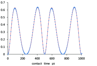
Figure 1: Comparison of CP dynamics derived from the analytical solution (solid line) and QCNMR (solid circles) with the conditions: $\omega_{1I}/2\pi=\omega_{1S}/2\pi$=80kHz and heteronuclear dipolar constant $d/\pi$=5kHz.

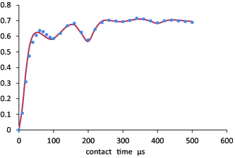
Figure 2: CP dynamics from a powder sample of alanine derived from the analytical solution (solid line) and experiments with the conditions: $R^{-1}=290.8\mu sec,\ R_{1}^{-1}=137.9\mu sec,\ T_{1\rho}=1.867msec,\ \omega_{1I}/2\pi=\omega_{1S}/2\pi$=80kHz, and the distance between ¹H and ¹³C spin is 1.09Å CH_distance . The experiment was done by Bruker Avance 300MHz NMR Instrument.

The CP dynamics with a MAS speed of 2 kHz is shown in FIG.1. It appears to be periodic with a period which is the same as the period of MAS ($T=2\pi/\omega_{r}$). The polarization of initial buildup and two nulls within the period ($T=500us$) are caused by the interference between dipolar oscillation and MAS. This pattern is unique in slow MAS speed. In the above calculation $R,\ R_{1}$, and $T_{1\rho}$ in the equation are all neglected for better comparison between theory and simulation.

In FIG.2, we show the dynamics of a powder sample under a MAS speed of 5 kHz. Unlike a single crystal, the oscillation is strongly damped by the orientations of heteronuclear dipolar tensors. The polarization increases gradually as the CP and spin diffusion take place. The experiment results are normalized according to quantitative CP experiment with a reciprocity relation Shujie ; Shuwenfang , while the solid line is normalized by the Eq. (14). In this case the match of two curves depends not only on the patterns but also on the specific values as well.

It can be seen from FIG.1 and FIG.2, all the simulated results agree well with the analytical solutions, demonstrating the validity of the analytical solution. The only approximation in the derivation is $|\omega_{1I}+\omega_{1S}|\gg|d(t)|$, which is well fulfilled in practice.

IV 4. Conclusion

Under Hartman-Hahn match condition, CP dynamics can be derived analytically in the zero- and double-quantum spaces. The solution is valid for any MAS speed and offsets. In particular, the dynamics for a stationary sample appears when MAS speed approaches zero. As many other methods, the CP dynamics provides valuable molecular structural information. Similar to REDO experiment REDO , this analytic solution also provides a measure of dipolar coupling constant(or distance) for a strongly coupled system that is surrounded by a moderately coupled network. Unlike many other others  Vega ; MeiHong ; F_Si ; C_H ; H_P ; F_C , this method does not required high MAS speed. If LG spin locking is applied to proton channel, the result of Least-Square fitting in FIG.2 will be better because all homonuclear coupling is decoupled.

For a time dependent system, it is unlikely to find a systematic way for analytic solutions. This may explain why CP dynamics discussed in this article was delayed for so long a time. For an inhomogeneously broaden system ($[\mathcal{H}(t^{\prime}),\mathcal{H}(t^{\prime\prime})]=0$) Broaden , all high order average Hamiltonians become zero except for the zero order average Hamiltonian that can be calculate conveniently. This method is quite general and can be used in NMR, optics, quantum computing and quantum mechanic related problems of a similar nature.

V acknowledgment

This work is supported by National Fundamental Research Project of China (2007CB925200). Peng Li is grateful ”PhD Program Scholarship Fund of ECNU 2007”. Qun Chen is grateful for ”Shanghai Leading Talent Training Program” and the support from Shanghai Committee of Science and Technology (11JC1403600).

References

- (1) S. Hartmann, E. L. Hahn, Phys. Rev. 44, 128 (1962) 2042.
- (2) A. Pines, M. S. Gibby, J. S. Waugh, J. Chem. Phys. 392, 61 (1974) 1255.
- (3) Lucaino Müller, Anil Kumar, Thomas Baumann, Richart R. Ernst, Phys. Rev. Lett. 32, 25(1974) 1402.
- (4) E. O. Stejskal, Jacob Schaefer, J. S. Waugh, J. Magn. Reson. 28, 105(1974) .
- (5) Shanmin Zhang, Corinnal L. Czekaj, Warren T. Ford, J. Magn. Reson. Series A 111, 1(1994) 87.
- (6) Lee. M., Goldburg. W. I., Phys. Rev. 140, 4A(1965) A1261.
- (7) Vladimir Ladizhansky and Shimon Vega, J. Chem. Phys. 112, 16(1974) 7158.
- (8) B. -J. van Rossum, C. P. de Groot, V. Ladizhansky, S. Vega, and H. J. M. de Groot, J. Am. Chem. Soc. 122, 14(2000) 3465.
- (9) Michael Mehring, High Resolution NMR in Solids (Springer-Verlag, Berlin Heidelberg New York,1983).
- (10) Goldman, M., Spin Temperature and Nuclear Magn. Res. in Solids. (Oxford Univ. Press 1970).
- (11) Waclaw Kolodziejski, and Jacek Klinowski, Chem. Rev 102, 3(2002) 613-628.
- (12) M. H. Levitt, D. Suter, R. R. Ernst, J. Chem. Phys. 84, 8(1986) 4243.
- (13) Shanmin Zhang, B. H. Meier, S. Appelt, M. Mehring, R. R. Ernst, J. Magn. Reson. Series A 101, 1(1993) 60.
- (14) Shanmin Zhang, B. H. Meier, and R. R. Ernst, J. Magn. Reson. Series A 108, 1(1994) 30-37.
- (15) B. H. Meier, Chem. Phys. Lett. 188, 201(1992).
- (16) S. Hediger, B. H. Meier, Narayanan D. Kurur, G. Bodenhausen, and R. R. Ernst, Chem. Phys. Lett. 223, (1994) 283-288.
- (17) U. Haeberlen, J. S. Waugh, Phys. Rev. 175, 2(1968) 453.
- (18) M. Lehmann, T. Koetzle, W. Hamilton, J. Am, Chem. Soc. 94, 8(1972) 2657.
- (19) J. Shu, Q. Chen, Shanmin Zhang, Chem. Phys. Lett. 462, 125(2008).
- (20) Wenfang Shu, Shanmin Zhang, Chem. Phys. Lett. 511, 424(2011).
- (21) T. Gullion and J. Schaefer, J. Magn. Reson. 81, 196(1989).
- (22) Mei Hong, Xiaolan Yao, Karen Jakes, and Daniel Huster, J. Phys. Chem. B 106, 29(2002) 7355.
- (23) Philippe Bertani, Jésus Raya, Pierre Reinheimer, Régis Gougeon, Luc Delmotte, Jérôme Hirschinger, Solid State Nucl. Magn. Reson. 13, (1999) 219-229.
- (24) Jiri Brus, Jaromír Jake, Solid State Nucl. Magn. Reson. 27, (2005) 180-191.
- (25) Maggy Hologen, Philippe Bertani, Thierry Azas, Christian Bonhomme, Jérôme Hirschinger, Solid State Nucl. Magn. Reson. 28, (2005) 50-56.
- (26) Jérôme Giraudet, Marc Dubois, Katia Guérin, Céline Delabarre, Pascal Pirotte, André Hamwi, Francis Masin, Solid State Nucl. Magn. Reson. 31, (2007) 131-140.
- (27) M. Matti Maricq and J. S. Waugh, J. Chem. Phys. 70, 3300(1979).