Molecular dynamics simulation of orientational glass formation in anisotropic particle systems in three dimensions

Abstract

We propose a simple microscopic model of molecular dynamics simulation to study orientational glass in three dimensions. We present simulation results for mixtures of mildly anisotropic particles and spherical impurities. We realize fcc solids without orientational order in a rotator phase. As the temperature $T$ is lowered, the disordered matrix is gradually replaced by four kinds of orientationally ordered, rhombohedral domains. Two-phase coexistence is realized in a temperature window. The impurities serve to anchor the orientations of the surrounding anisotropic particles, resulting in finely divided domains or medium long-range orientational order. We examine the rotational dynamics of the molecular orientations which is slowed down at low $T$. We predict the shape memory effect under a stretching cycle due to inter-variant transformation.

1 Introduction

Nonspherical molecules such as KCN can form a crystal without long-range orientational order for mild molecular anisotropy [1], while liquid crystal phases can appear for large molecular anisotropy. Such crystals are called plastic crystals in a rotator phase. They undergo an orientational phase transition as the temperature $T$ is further lowered, where the crystal structure is cubic at high $T$ and non-cubic at low $T$. With inclusion of impurities in such solids, the so-called orientational glass has been realized [1]. Around the transitions, a peak in the specific heat [1] and softening of the shear modulus [1, 2] have been observed. In real systems, the molecules often have dipolar moments, yielding dielectric anomaly. As a similar example, metallic ferroelectric glass, called relaxor, has been studied extensively [3], where frozen polar nanodomains have been observed.

For one-component anisotropic particle systems, there have been a number of simulations on the statics [4, 5, 6, 7, 8, 9, 10] and dynamics [11, 12] of the orientational phase transition. For two-component anisotropic particle systems, Chong et al. examined the slowing-down of the orientational time-correlation functions around the glass transition [13]. In this paper, setting up a simple microscopic model, we will investigate the formation of orientational glass. In particular, we will examine how impurities can microscopically produce orientational disorder, which has remained unexplored in the literature. Furthermore, alignments of anisotropic particles formig a crystal give rise to lattice deformations. As a unique feature in orientational glass, heterogeneous strains should emerge on mesoscopic scales. In such situations, we may predict soft elasticity and a shape memory effect against applied stress.

2 Model

We consider a binary mixture of anisotropic particles with number $N_{1}$ and spherical particles with number $N_{2}$. In this paper, we set $N_{1}+N_{2}=8192$. The composition of the second species is defined by

$$c=N_{2}/(N_{1}+N_{2}).$$ (1)

We assume relatively small $c$, so the spherical particles may be treated as impurities. The particle positions are written as ${\mbox{\boldmath$r$}}_{i}$ ($i=1,\cdots,N$). The anisotropic particles are assumed to be axisymmetric; then, their orientation may be expressed in terms of the solid angles $\phi_{i}$ and $\theta_{i}$ ($i=1,\cdots,N_{1}$) as ${\mbox{\boldmath$n$}}_{i}=(\sin\theta_{i}\sin\phi_{i},\sin\theta_{i}\cos\phi_{i},\cos\theta_{i}).$ The particle sizes of the two species are characterized by lengths $\sigma_{1}$ and $\sigma_{2}$. The pair potential $U_{ij}$ between particles $i\in\alpha$ and $j\in\beta$ ($\alpha,\beta=1,2$) is a truncated modified Lennard-Jones potential depending on the particle distance $r_{ij}=|{\mbox{\boldmath$r$}}_{i}-{\mbox{\boldmath$r$}}_{j}|$ and the directions ${\mbox{\boldmath$n$}}_{i}$ and ${\mbox{\boldmath$n$}}_{j}$. For $r_{ij}>r_{c}=3\sigma_{1}$ it is zero, while for $r_{ij}<r_{c}=3\sigma_{1}$ it reads

$$U_{ij}=4\epsilon\bigg{[}(1+A_{ij})\frac{\sigma^{12}_{\alpha\beta}}{r_{ij}^{12}}-\frac{\sigma_{\alpha\beta}^{6}}{r_{ij}^{6}}\bigg{]}-C_{ij},$$ (2)

where $\epsilon$ is the characteristic interaction energy and

$$\sigma_{\alpha\beta}=(\sigma_{\alpha}+\sigma_{\beta})/2.$$ (3)

The particle anisotropy is taken into account by the angle factor $A_{ij}$, which depends on the relative direction $\hat{\mbox{\boldmath$r$}}_{ij}=r_{ij}^{-1}({\mbox{\boldmath$r$}}_{i}-{\mbox{\boldmath$r$}}_{j})$ and the orientations ${\mbox{\boldmath$n$}}_{i}$ and ${\mbox{\boldmath$n$}}_{j}$. In this paper, we assume the following form,

$$A_{ij}=\chi\delta_{\alpha 1}({\mbox{\boldmath$n$}}_{i}\cdot\hat{\mbox{\boldmath$r$}}_{ij})^{2}+\chi\delta_{\beta 1}({\mbox{\boldmath$n$}}_{j}\cdot\hat{\mbox{\boldmath$r$}}_{ij})^{2},$$ (4)

where $\chi$ is the anisotropy strength of repulsion. The $\delta_{\alpha 1}$ ($\delta_{\beta 1}$) is equal to 1 for $\alpha=1$ $(\beta=1$) and 0 for $\alpha=2$ ($\beta=2$). In the right hand side, the first (second) term is nonvanishing only when $i$ ($j$) belongs to the first species. The $C_{ij}$ ensures the continuity of $U_{ij}$ at $r=r_{c}$.

In our system, the total potential energy is the sum $U=\sum_{1\leq i<j\leq N}U_{ij}$, while the total kinetic energy $K$ arises from the translational velocity ${\dot{\mbox{\boldmath$r$}}}_{i}=d{\mbox{\boldmath$r$}}_{i}/dt$ and the rotational velocity ${\dot{\mbox{\boldmath$n$}}}_{i}=d{\mbox{\boldmath$n$}}_{i}/dt$ as

$$K=\sum_{1\leq i\leq N}\frac{1}{2}m_{\alpha}|{\dot{\mbox{\boldmath$r$}}}_{i}|^{2}+\sum_{1\leq i\leq N_{1}}\frac{1}{2}I_{1}|{\dot{\mbox{\boldmath$n$}}}_{i}|^{2},$$ (5)

where $m_{1}$ and $m_{2}$ are the masses, and $I_{1}$ is the moment of inertia of the first species. We set $m_{1}=m_{2}$ in our simulation. The molecular rotation around the symmetry axis parallel to ${\mbox{\boldmath$n$}}_{i}$ does not change $U$, so we may neglect its kinetic energy. The Newton equations of motion for translation and rotation are written as [14]

$${m_{\alpha}}{\ddot{\mbox{\boldmath$r$}}}_{i}=-\frac{\partial{U}}{\partial{{\mbox{\boldmath$r$}}_{i}}}\quad(i=1,\cdots,N),$$ (6)

$$I_{1}{\mbox{\boldmath$n$}}_{i}\times{\ddot{\mbox{\boldmath$n$}}}_{i}=-{\mbox{\boldmath$n$}}_{i}\times\frac{\partial{U}}{\partial{{\mbox{\boldmath$n$}}_{i}}}\quad(i=1,\cdots,N_{1}),$$ (7)

where ${\ddot{\mbox{\boldmath$r$}}}_{i}={d^{2}}{\mbox{\boldmath$r$}}_{i}/{dt^{2}}$ and ${\ddot{\mbox{\boldmath$n$}}}_{i}={d^{2}}{\mbox{\boldmath$n$}}_{i}/{dt^{2}}$. Hereafter, we measure space, time, and temperature in units of $\sigma_{1}$, $\tau_{0}=\sigma_{1}\sqrt{m_{1}/\epsilon},$ and $\epsilon/k_{B}$, respectively.

Treating equilibrium or at least nearly steady states, we furthermore attach a Nos$\acute{\rm e}$-Hoover thermostat [15] to all the particles. That is, we added the thermostat terms $-\zeta_{\rm NH}(t)m_{\alpha}{\dot{\mbox{\boldmath$r$}}}_{i}$ and $-\zeta_{\rm NH}(t)I_{1}{\mbox{\boldmath$n$}}_{i}\times{\dot{\mbox{\boldmath$n$}}}_{i}$ in the right hand sides of Eqs.(6) and (7), respectively, where $\zeta_{\rm NH}(t)$ obeys

$$\tau_{\rm NH}^{2}\frac{d}{dt}{\zeta_{\rm NH}(t)}=-1+K/[k_{B}T(3N/2+N_{1})],$$ (8)

with $\tau_{\rm NH}$ being a short relaxation time taken to be 0.1.

We may envisage the anisotropic particles as spheroids depending on the parameter $\chi$ from Eq.(4). For particles $i$ and $j$ of the first species, minimization of $U_{ij}$ with respect to $r_{ij}$ yields $r_{ij}=2^{1/6}(1+A_{ij})^{1/6}\sigma_{1}$. For $\chi>0$, the short and long diameters, $a_{s}$ and $a_{\ell}$, are given by

$$a_{s}=2^{1/6}\sigma_{1},\quad a_{\ell}=(1+2\chi)^{1/6}2^{1/6}\sigma_{1},$$ (9)

for the perpendicular and parallel orientations of ${\mbox{\boldmath$n$}}_{i}$ and ${\mbox{\boldmath$n$}}_{j}$ with respect to ${\hat{\mbox{\boldmath$r$}}}_{ij}$, respectively. The inertia momentum of the first species in Eq.(7) is given by

$$I_{1}=(a_{\ell}^{2}+a_{s}^{2})m_{1}/20.$$ (10)

In our simulation, we set $\sigma_{2}/\sigma_{1}=1.1$ and $\chi=1.2$. From Eq.(9) the aspect ratio is $a_{\ell}/a_{s}=1.23$. For these mild parameter values, we realized fcc plastic solids without long-range orientational order at relatively high $T$. For large $\chi$, say 10, we realized liquid crystal phases in our model. It is worth noting that our angle-dependent potential (2) is analogous to the Gay-Berne potential for anisotropic molecules used to simulate mesophases of liquid crystals [16]. Similar angle-dependent potentials have also been used for lipids forming membranes. [17, 18].

3 Four-variant states at fixed volume

Starting with liquid states at $T=2$, we quenched the system to $T=0.5$ below the melting and waited for $10^{4}$ to realize fcc plastic crystals. Here, a few stacking faults were formed in most runs. We then cooled the system to a final temperature and waited for $3\times 10^{4}$, where orientational order developed. In Figs.1-7, we fixed the system volume and shape imposing the periodic boundary condition. In terms of the molecular volumes $v_{1}=\pi a_{s}^{2}a_{\ell}/6$ and $v_{2}=\pi 2^{1/2}\sigma_{2}^{3}/6$, the packing fraction $\phi_{\rm pack}$ is given by

$$\phi_{\rm pack}=(N_{1}v_{1}+N_{2}v_{2})/V.$$ (11)

We set $\phi_{\rm pack}=0.82$ in Figs.1-7. Then the system length is about $20$ and the pressure is about $4\epsilon/\sigma_{1}^{3}$.

F1.pdf

Figure 1: Frozen domain structures composed of four rhombohedral variants for $\sigma_{2}/\sigma_{1}=1.1$, $\chi=1.2$, and $T=0.1$ at fixed volume. With increasing the composition $c$ of the impurities (black points), the orientational disorder increases, leading to a decrease in the domain size. The particle color is blue, green, and red for ${\mbox{\boldmath$n$}}_{i}=(\pm 1,0,0)$, $(0,\pm 1,0)$, $(0,0,\pm 1)$, respectively.

F2.pdf

Figure 2: Anchoring of spheroidal particles around a single impurity (left) and two associated impurities (right) for $\sigma_{2}/\sigma_{1}=1.1$, $\chi=1.2$, and $T=0.1$.

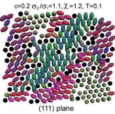
Figure 3: Crosssectional snapshot in a (111) plane, where four rhombohedral domains composed of spheroidal particles can be seen with impurities (black) disturbing the orientations. Here, $c=0.2$, $\sigma_{2}/\sigma_{1}=1.1$, $\chi=1.2$, and $T=0.1$ .

F4.pdf

Figure 4: Snapshots of impurities composing clusters with sizes $\geq 5$ for $c=0.1$ (left) and for $c=0.2$ (right) with mesoscopic heterogeneities. The data are the same as those in Fig.1.

In Fig.1, the orientational domains can be seen at $T=0.1$, where the particle positions and orientations are nearly frozen in time. For $c=0$, the system undergoes a structural phase transition, where the lattice structure changes from fcc to rhombohedral almost without dilation change. The lattice constant is equal to $a=1.65$ through the transition. The ordered phase consists of four rhombohedral variants where the angles of the rhombuses are $83^{\circ}$ and $97^{\circ}$. The separation distance of the closely packed $(111)$ planes is increased from $a/\sqrt{3}=0.952$ to 1.08, because the orientation vectors ${\mbox{\boldmath$n$}}_{i}$ are aligned in the $[111]$ direction. With increasing $c$, the orientational disorder is gradually increased, leading to pinning of finely divided domains. We eventually obtain a glass state at $c=0.3$.

In Fig.2, the anisotropic particles are aligned in the perpendicular directions $(\perp{\hat{\mbox{\boldmath$r$}}}_{ij}$) around one or two impurities. This parallel anchoring disturbs the orientation order. In Fig.3, in a (111) plane, we display the four rhombohedral variants with different orientations for $c=0.2$. The interfaces between the variants tend to be trapped at clustered impurities. We also notice that the junction angles, at which two or more domain boundaries intersect, are approximately multiples of $\pi/6$. Similar patterns were observed on hexagonal planes in a number of experiments on alloys after structural phase transitions [19].

4 Impurity clustering

Figure 4 shows significant impurity clustering, which appeared during quenching from liquid. The average impurity number per cluster is 5.5 for $c=0.1$ and there is a big percolated cluster for $c=0.2$. Here, two impurities are treated to belong to the same cluster if their distance is smaller than 1.3. In the snapshot of $c=0.3$ in Fig.1, the impurity clustering is closely related to the heterogeneity in the orientations.

To explain this effect, we compare the solvation energy of a single impurity and that of two associated impurities (see Fig.2). In terms of the potential energy $U_{j}=\sum_{k}U_{jk}/2$ of particle $j$, it is estimated as

$$U_{\rm sol}=U_{\rm imp}+\sum_{{\rm nearby}~{}j\in 1}(U_{j}-\bar{U}_{1}).$$ (12)

Here, $U_{\rm imp}$ is the contribution from the impurities under consideration, the summation is over the nearby anisotropic particles $j$ with $r_{ij}<1.3$ ($i\in 2$ and $j\in 1$), and $\bar{U}_{1}$ is the average potential energy of the non-neighbor anisotropic particles separated from any impurities longer than $1.3$. At $T=0.1$, $U_{\rm sol}$ is calculated as $U_{\rm sol}^{(1)}=-6.3\epsilon$ for a single impurity and $U_{\rm sol}^{(2)}=-13.8\epsilon$ for a dimer, where $\bar{U}_{1}\cong-4.5\epsilon$. The difference $\Delta U_{\rm sol}=U_{\rm sol}^{(2)}-2U_{\rm sol}^{(1)}(\sim-1.2\epsilon)$ is the association energy. At $T=0.25$, we have $\Delta U_{\rm sol}\sim-1.8\epsilon$. The total potential energy is thus lowered with impurity clustering in the present case.

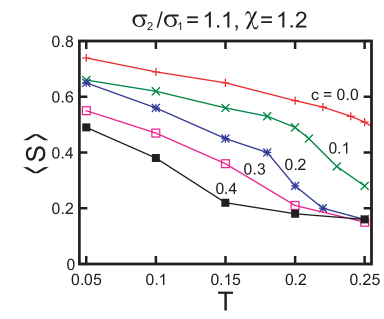
Figure 5: $\langle{S}\rangle=\sum_{i\in 1}S_{i}/N_{1}$ vs $T$, for $c=0,0.1,0.2,0.3$, and 0.4 for $\sigma_{2}/\sigma_{1}=1.1$, and $\chi=1.2$. This quantity represents the overall degree of orientational order.

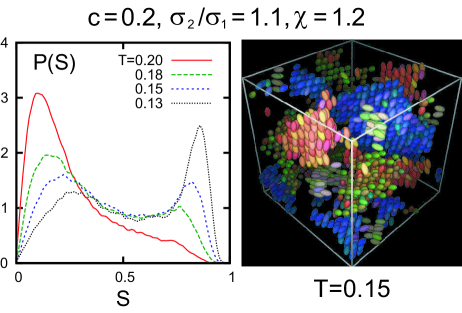
Figure 6: Left: Distribution of the orientation amplitude $P(S)$ in Eq.(15) for various $T$, where $c=0.2$, $\sigma_{2}/\sigma_{1}=1.1$, and $\chi=1.2$. It exhibits double peals for $T=0.13$, 0.15, and 0.18 representing coexistence of cubic and rhombohedral regions. Right: Snapshot of anisotropic particles with $S_{i}>0.6$ at $T=0.15$, forming ordered domains embedded in a disordered matrix.

5 Coarse-grained orientation order parameter

For each particle $i$ of the first species, we introduce the orientation tensor ${\stackrel{{\scriptstyle\leftrightarrow}}{{Q}}}_{i}=\{Q_{i\mu\nu}\}$ ($\mu,\nu=x,y,z$) as

$$\stackrel{{\scriptstyle\leftrightarrow}}{{Q}}_{i}=\frac{1}{1+n_{\rm b}^{i}}\bigg{(}{\mbox{\boldmath$n$}}_{i}{\mbox{\boldmath$n$}}_{i}+\sum_{j\in{\rm bonded}}{\mbox{\boldmath$n$}}_{j}{\mbox{\boldmath$n$}}_{j}\bigg{)}-\frac{1}{3}\stackrel{{\scriptstyle\leftrightarrow}}{{1}},$$ (13)

where ${\stackrel{{\scriptstyle\leftrightarrow}}{{1}}}=\{\delta_{\mu\nu}\}$ is the unit tensor. The summation is over the bonded particles of the first species with $|{\mbox{\boldmath$r$}}_{ij}|<1.5\sigma_{1}$ and $n_{\rm b}^{i}$ is the number of these particles. If a fcc lattice is formed, it includes the nearest neighbor particles, so $n_{\rm b}^{i}\sim 12$. We define the amplitude of the orientational order for each anisotropic particle $i$ as

$${S_{i}}={\frac{3}{2}}\sum_{\mu,\nu}Q_{i\mu\nu}^{2}.$$ (14)

Here, $S_{i}\sim 0.1$ in disordered regions due to the thermal fluctuations, but it increases up to unity within rhombohedral domains at low $T$. In Fig.5, the average $\langle{S}\rangle=\sum_{1\leq i\leq N_{1}}S_{i}/N_{1}$ represents the overall degree of orientation order. In our simulation, we realized only uniaxial states, where we have $\stackrel{{\scriptstyle\leftrightarrow}}{{Q}}_{i}=S_{i}^{1/2}({\mbox{\boldmath$d$}}_{i}{\mbox{\boldmath$d$}}_{i}-\stackrel{{\scriptstyle\leftrightarrow}}{{1}}/3)$ in terms of the amplitude $S_{i}$ and the director ${\mbox{\boldmath$d$}}_{i}$.

6 Coexistence of high and low temperature phases

In Fig.5, the degree of orientational order $\langle{S}\rangle$ increases continuously as $T$ is lowered. For small $c$ at fixed volume and shape, however, we find coexistence of cubic and rhombohedral regions in a temperature window, which is roughly given by $0.26<\kern-12.0pt\lower 5.0pt\hbox{$\displaystyle{\sim}$}T<\kern-12.0pt\lower 5.0pt\hbox{$\displaystyle{\sim}$}0.29$ for $c=0$ and $0.14<\kern-12.0pt\lower 5.0pt\hbox{$\displaystyle{\sim}$}T<\kern-12.0pt\lower 5.0pt\hbox{$\displaystyle{\sim}$}0.19$ for $c=0.2$. To examine this coexistence, we introduce the distribution of the orientational amplitude,

$$P(S)=\frac{1}{N_{1}}\sum_{1\leq i\leq N_{1}}\langle{\delta(S-S_{i})}\rangle.$$ (15)

Taking the average $\langle{\cdots}\rangle$ over six runs we obtained $P(S)$ in Fig.6, which exhibits two peaks for $0.13\leq T\leq 0.18$ at $c=0.2$. We also give a snapshot of the ordered anisotropic particles with $S_{i}>0.6$. For $c=0$, the interfaces between the ordered and disordered regions are temporally fluctuating with small amplitudes. Small amounts of impurities can pin the interfaces and the ordered regions are stabilized far from the impurity clusters.

7 Rotational dynamics

In crystal and glass, elongated particles often undergo turnover motions, ${\mbox{\boldmath$n$}}_{i}\to-{\mbox{\boldmath$n$}}_{i}$. These events take place in a microscopic time $(\sim 1$), while the characteristic time $\tau_{1}$ between successive turnover motions grows at low $T$. Let us consider the following angle relaxation function,

$$W(\zeta,t)=\frac{1}{N_{1}}\sum_{1\leq i\leq N_{1}}\bigg{\langle}{\delta(\zeta-{\mbox{\boldmath$n$}}_{i}(t+t_{0})\cdot{\mbox{\boldmath$n$}}_{i}(t_{0}))}\bigg{\rangle},$$ (16)

where the average $\langle{\cdots}\rangle$ is taken over the initial time $t_{0}$ and over six runs in this paper. Furthermore, in terms of the $\ell$-th order Legendre polynomials $P_{\ell}$, we may define the $\ell$-th order rotational relaxation functions as [11, 12, 13]

$$C_{\ell}(t)=\int_{-1}^{1}d\zeta P_{\ell}(\zeta)W(\zeta,t).$$ (17)

Here $C_{1}(t)$ decays on the timescale of $\tau_{1}$, while $C_{2}(t)$ is unchanged by the turnover motions. In orientational glass, the ultimate relaxation of $C_{2}(t)$ is due to the orientational configuration changes involving the surrounding particles, so its relaxation time $\tau_{2}$ much exceeds $\tau_{1}$.

Figure 7: Orientation relaxation functions $C_{1}(t)$ in (a) and $C_{2}(t)$ in (b) for $c=0.2$, $\sigma_{2}/\sigma_{1}=1.1$, and $\chi=1.2$. $C_{1}(t)$ decays due to turnover motions and its relaxation time $\tau_{1}$ is marked on each curve (see Eq.(19)). $C_{2}(t)$ can relax only due to the orientational configuration changes. (c) Distribution $W(\zeta,t)$ in Eq.(16) and (d) turnover fraction in Eq,(18) at three times.

In Fig.7, we plot $C_{1}(t)$ and $C_{2}(t)$ vs $t$ for $c=0.2$. For $t<\kern-12.0pt\lower 5.0pt\hbox{$\displaystyle{\sim}$}1$ they relax considerably due to the thermal motions. The decay of $C_{1}(t)$ is slower for lower $T$, while $C_{2}(t)$ apparently tends to a positive constant $f_{2}$ for large $t$, as in the previous simulation [13]. In our case, this plateau appears because the anchoring of the anisotropic particles around the impurities becomes nearly permanent at low $T$. Thus $f_{2}$ increases with lowering $T$. In Fig.7, we also present the time-evolution of the relaxation function $W(\zeta,t)$ for $t=200,2000$, and 20000, which is peaked at $\zeta=\pm 1$. The peak height at $\zeta=-1$ increases in time from 0. Also shown is the turnover probability defined by

$$W_{\rm to}(t)=\int_{-1}^{-1+\Delta\zeta}d\zeta~{}W(\zeta,t),$$ (18)

where we set $\Delta\zeta=0.2$. We notice that $W_{\rm to}(t)$ grows linearly in time in the very early stage. Thus we may define $\tau_{1}=\tau_{1}(T)$ from the following linear form,

$$W_{\rm to}(t)\cong\tau_{1}^{-1}t,$$ (19)

which holds for $t/\tau_{1}<\kern-12.0pt\lower 5.0pt\hbox{$\displaystyle{\sim}$}0.1$. For $0.1<\kern-12.0pt\lower 5.0pt\hbox{$\displaystyle{\sim}$}t/\tau_{1}<\kern-12.0pt\lower 5.0pt\hbox{$\displaystyle{\sim}$}1$, the probability of multiple turnovers becomes appreciable resulting in a deviation from the linear behavior (19). However, the scaling form $W_{\rm to}(t)=f_{\rm to}(t/\tau_{1})$ fairly holds for $t/\tau_{1}<1$. For $t/\tau_{1}>\kern-12.0pt\lower 5.0pt\hbox{$\displaystyle{\sim}$}4$, the orientational structural relaxation comes into play and the scaling in terms of $\tau_{1}$ does not hold.

8 Shape memory effect

In the presence of multi-variant orientational order, the shape-memory effect (mechanical hysteresis) emerges almost without dislocation formation. This effect is well-known for shape memory alloys such as Ti-Ni [20], where a structural phase transition is caused by the relative atomic displacements in each unit cell. In our case, under stretching along the $z$ axis, domains with ${\mbox{\boldmath$n$}}_{i}$ nearly parallel to the $z$ axis grow yielding an increase in the strain. We are not aware of any experiments on this effect in anisotropic particle systems.

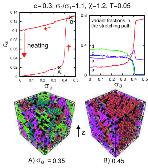
Figure 8: Shape memory effect under stretching along the $z$ axis in orientational glass with $c=0.3$ in stress-controlled simulation, where $T=0.05$, $\sigma_{2}/\sigma_{1}=1.1$, and $\chi=1.2$. Top left: Strain $\varepsilon_{z}$ vs stress ${\sigma_{a}}$, where $\varepsilon_{z}$ increases slowly in the hard ranges $0<\sigma_{a}<0.38$ and $0.42<\sigma_{a}<0.5$ and steeply in the soft range $0.38<\sigma_{a}<0.42$. The return path is reversible with large Young’s modulus. After this cycle, the residual strain is $0.1$, which vanishes upon heating to $T=0.2$. Top right: Time-evolution of four variant fractions on the stretching path. For $\sigma_{a}>0.38$ the two variants with their orientations ${\mbox{\boldmath$n$}}_{i}$ nearly parallel to the $z$ axis become dominant. Bottom: Snapshots of the particle configurations at (A) $\sigma_{a}=0.35$ and (B) $\sigma_{a}=0.45$.

In this mechanical effect, the system shape changes. Thus we assumed a Parrinello-Rahman barostat [14, 21] as well as the Nos$\acute{\rm e}$-Hoover thermostat. Before streching we prepared a multi-variant initial state at $t=0$, where the packing fraction $\phi_{\rm pack}$ in Eq.(11) was 0.75 and the pressure was zero. For $t>0$ we applied the stress $\sigma_{a}\equiv-\langle{\Pi_{zz}}\rangle,$ setting $\langle{\Pi_{xx}}\rangle=\langle{\Pi_{yy}}\rangle=0$, where $\Pi_{\mu\nu}$ are the stress components with $\langle{\cdots}\rangle$ being the space average. We allowed the system to take a rectangular shape. In terms of the system length $L_{z}(t)$ along the $z$ axis, the average strain is

$$\varepsilon_{z}=L_{z}(t)/L_{z}(0)-1.$$ (20)

We define effective Young’s modulus $E_{e}$ by $\partial\varepsilon_{z}/\partial\sigma_{a}=1/E_{e}$. It follows the effective shear modulus $\mu_{e}$ from the formula $E_{e}=3\mu_{e}/(1+\mu_{e}/3K)$ in classical elasticity, where $K$ is the bulk modulus. In our case $K$ is about $50$ and is much larger than $\mu_{e}$, so $E_{e}\cong 3\mu_{e}$. Hereafter, $\sigma_{a}$ and $E_{e}$ will be measured in units of $\epsilon/\sigma_{1}^{3}$.

In Fig.8, we first increased $\sigma_{a}$ at $d\sigma_{a}/dt=5\times 10^{-5}$ from 0 up to 0.5 at $T=0.05$. In the left panel, we find $E_{e}\sim 17$ for $0<\sigma_{a}<0.38$, $E_{e}\sim 3$ for $0,38<\sigma_{a}<0.42$, and $E_{e}\sim 20$ for $0,42<\sigma_{a}<0.5$. In the second range, the solid is soft because the variants elongated along the $z$ axis grow due to inter-variant transformation. Here, the orientation vectors ${\mbox{\boldmath$n$}}_{i}=(n_{ix},n_{iy},n_{iz})$ of the four variants are roughly given by (a) (0.3,-0.1,0.9), (b) (-0.7,0.1,0.7), (c) (0.7,0.7,0.2), and (d) (0.5,-0.9,0.1) in Fig.8. In the right panel, the variant (a) grows, the variant (b) remains nonvanishing, and the variants (c) and (d) disappear. Secondly, we decreased $\sigma_{a}$ back to 0 at $d\sigma_{a}/dt=-5\times 10^{-5}$. In this return path, $E_{e}$ was about $20$, the disfavored variants no more appeared, and a remnant strain of order $0.1$ remained. Thirdly, at $\sigma_{a}=0$, we increased $T$ from 0.05 to 0.2 into the disordered phase. After this heating, the system became isotropic.

9 Summary

We have siudied the orientational glass using the potential (2). Due to the anisotropic factor $A_{ij}$, the anisotropic particles have the aspect ratio $(1+2\chi)^{1/6}$. In our simulation, the anisotropy parameter $\chi$ is 1.2 and the size ratio $\sigma_{2}/\sigma_{1}$ is 1.1. As a result, fcc plastic crystals appear at relatively high $T$, which undergo the orientation transition at lower $T$. The impurities serve to pin the orientations of the surrounding anisotropic particles.

We briefly summarize our main results. In Fig.1, we have illustrated four-variant ordered states for various $c$ at $T=0.1$. With increasing $c$, rhombohedral domains are finely divided and their typical size is decreased. In Fig.4, we have shown that the impurities are heterogeneously distributed. In Fig.5, we have plotted the average orientational amplitude $\langle{S}\rangle$, which increases continuously with lowering $T$. In Fig.6, we have shown large-scale coexistence of the disordered and ordered phases in a temperature window. In Fig.7, the orientational time-correlation functions have been plotted for $c=0.2$, where $C_{1}(t)$ decays due to turnover motions. In Fig.8, we have examined the shape memory effect in orientational glass.

We next make some remarks below.
(i) For small $c$, we need to know how the characteristic domain size is determined. For moderate impurity concentrations ($c>\kern-12.0pt\lower 5.0pt\hbox{$\displaystyle{\sim}$}0.2$ in this work), the orientational disorder is proliferated. These aspects should be further studied.

(ii) The phase transition delicately depends on whether simulations are performed at fixed volume or at fixed stress. Some salient features at fixed stress are as follows. (a) For $c=0$, a first-order phase transition occurs with a shape change. (b) For $c>0$, both multi-domain states and single-domain states can be realized for the same parameters as in Fig.8. (c) For $c>0$, the two-phase coexistence in Fig.6 can still be realized even at fixed stress.

(iii) In our simulation, the system keeps the crystalline order. However, for larger size ratio $\sigma_{2}/\sigma_{1}$, say 1.4, we found an increase in the positional disorder leading to polycrystal and positional glass. Competition of positional and orientational glass transitions can then be studied. For large anisotropic parameter $\chi$, we may also study complicated phase behavior of two-component liquid crystals.

(iv) In this paper, the impurities are spherical and slightly larger than the anisotropic particles. By modifying the potential form, we may also treat other types of impurities. For example, their attractive interaction with the host anisotropic particles may be anisotropic; then, the anchoring can be homeotropic.

- [1] \NameHöchli U. T., Knorr K. Loidl A. \REVIEWAdv. Phys.391990405.
- [2] \NameLynden-Bell R. M. Michel K. H. \REVIEWRev, Mod. Phys.661994721.
- [3] \NameVugmeister B. E. Glinchuk M. D. \REVIEWRev. Mod. Phys.621990993; \NameHirota K., Wakimoto S. Cox D. E. \REVIEWJ. Phys. Soc. Jpn.752006111006.
- [4] \NameFrenkel D. Mulder B. M. \REVIEWMol. Phys.5519851171; \NameVeerman J. A. C. Frenkel D. \REVIEWPhys. Rev. A4119903237; \NameBolhuis P. Frenkel D. \REVIEWJ. Chem. Phys.1061997666.
- [5] \NameAllen M. P. Imbierski A. A. \REVIEWMol. Phys.601987453.
- [6] \NameSinger S. J. Mumaugh R. \REVIEWJ. Chem. Phys.9319901278.
- [7] \NameVega C., Paras E. P. A. Monson P. A. \REVIEWJ. Chem. Phys.9619929060; \SAME9719928543.
- [8] \NameRadu M., Pfleiderer P. Schilling T. \REVIEWJ. Chem. Phys.1312009164513.
- [9] \NameMcGrother S. C., Williamson D. C. Jackson G. \REVIEWJ. Chem. Phys.10419966755.
- [10] \NameMarechal M. Dijkstra M. \REVIEWPhys. Rev. E772008061405.
- [11] \NameDe Michele C., Schilling R. Sciortino F. \REVIEWPhys. Rev. Lett.982007265702.
- [12] \NameCaballero N. B., Zuriaga M., Carignano M. Serra P. \REVIEWJ. Chem. Phys.1362012094515.
- [13] \NameChong S.-H., Moreno A. J., Sciortino F. Kob W. \REVIEWPhys. Rev. Lett.942005215701; \NameChong S.-H. Kob W. \REVIEWPhys. Rev. Lett.1022009025702.
- [14] \NameAllen M. P. Tildesley D. J. \BookComputer Simulation of Liquids \PublClarendon Press, Oxford \Year1987.
- [15] \NameNosé S. \REVIEWMol. Phys.521984255.
- [16] \NameGay J. G. Berne B. J. \REVIEWJ. Chem. Phys.7419813316; \NameBrown J. T., Allen M. P., del Rio E. M. de Miguel E. \REVIEWPhys. Rev. E5719986685.
- [17] \NameDrouffe J.-M., Maggs A. C. Leibler S. \REVIEWScience25419911353.
- [18] \NameNoguchi H. \REVIEWJ. Chem. Phys.1342011055101.
- [19] \NameKitano Y., Kifune K. Komura Y. \REVIEWJ. Phys. (Paris)491988C5-201; \NameManolikas C. Amelinckx S. \REVIEWPhys. Stat. Sol. (a)601980607.
- [20] \NameSarkar S., Ren X. Otsuka K. \REVIEWPhys. Rev. Lett.952005205702; \NameWang Y., Ren X. Otsuka K. \REVIEWPhys. Rev. Lett.972006225703.
- [21] \NameParrinello M. Rahman A. \REVIEWJ. Appl. Phys.5219817182.