Distance weighted city growth

Abstract

Urban agglomerations exhibit complex emergent features of which Zipf’s law, i.e. a power-law size distribution, and fractality may be regarded as the most prominent ones. We propose a simplistic model for the generation of city-like structures which is solely based on the assumption that growth is more likely to take place close to inhabited space. The model involves one parameter which is an exponent determining how strongly the attraction decays with the distance. In addition, the model is run iteratively so that existing clusters can grow (together) and new ones can emerge. The model is capable of reproducing the size distribution and the fractality of the boundary of the largest cluster. While the power-law distribution depends on both, the imposed exponent and the iteration, the fractality seems to be independent of the former and only depends on the latter. Analyzing land-cover data we estimate the parameter-value $\gamma\approx 2.5$ for Paris and it’s surroundings.

I Introduction

Cities or urban agglomerations exhibit signatures of complex phenomena, such as broad size distributions Auerbach (1913); Zipf (2012); Saichev et al. (2010); Rozenfeld et al. (2011); Berry and Okulicz-Kozaryn (2012) and fractal structure Batty and Longley (1994, 1987) (and references therein). The last decades have witnessed a strong interest within the scientific community in characterizing the worldwide urbanization phenomenon. This line of research has strongly benefited from accessibility of demographic databases and from application of tools originated in statistical physics enabling the identification and analysis of universal aspects of urban forms and scaling features Bettencourt and West (2010). Beyond the descriptive level, various attempts to obtain insights into mechanisms that underly the complex features of cities have been proposed.

(i) Multiplicative models Levy and Solomon (1996); Gabaix (1999); Malcai et al. (1999); Gabaix (2009) have explored the connection between random city growth and city size distributions. In particular, building on discrete random walk theory, multiplicative models have proved successful at reproducing Zipf’s law (i.e. power-law city size distribution with exponent close to $2$). Furthermore, some of these models have proposed plausible explanations for the origin of these mechanisms, based on spatial economics theory Gabaix (1999). Notwithstanding this fact, multiplicative models are space-independent and thus are unable to address other important features of city structures, such as self-similarity. (ii) Approaches based on cellular automata have been used to model spatial structure of urban land use over time White and Engelen (1993) reproducing fractal properties. (iii) The correlated percolation model (CPM) Makse et al. (1995, 1998) assumes that an urban built environment is shaped by spatial correlations, where the occupation probabilities of two sites are more similar the closer they are. The model involves the empirical findings on the radial decay of density around a city center. For certain ranges in the space of parameters, the CPM reproduces basic features of real urban aggregates, such as broad size distributions in urban clusters and the fractal scaling of the perimeter. (iv) Reaction diffusion models Zanette and Manrubia (1997); Marsili et al. (1998); Zanette and Manrubia (1998) have been introduced in order to explore the role of intermittency in creating spatial inhomogeneities, in agreement with Zipf’s law. (v) Spatial explicit preferential attachment has been shown to be capable of reproducing Zipf’s law Schweitzer and Steinbrink (1998). Here, the probability that a city grows is essentially assumed to be proportional to the size of the city. (vi) Agent based modeling has been employed to simulate urban growth Schweitzer (2003), reproducing the formation of new clusters as well as the merging of neighboring ones. (vii) A random group formation is presented in Baek et al. (2011) from which a Bayesian estimate is obtained based on minimal information. It represents a general approach for power-law distributed group sizes.

While the term demographic gravitation was coined by Stewart (1948), in geographical economics, gravitational models have been investigated for many decades. Carrothers (1956) provides a review of gravity and potential concepts of human interaction. The so-called Reilly’s law of retail gravitation describes the breaking point of the boundary of equal attraction Reilly (1931). Similarly, Huff’s law of shopper attraction Huff (1963) provides the probability of an agent at a given site to travel to a particular facility. Last but not least, the volume of trade between countries has been described from the point of view of gravity analogy Poyhonen (1963). In contrast, limitation of gravitational models have been pointed out in the context of mobility and migration Simini et al. (2012).

Following the first law of geography ”Everything is related to everything else, but near things are more related than distant things” Tobler (1970), we elaborate on the role of gravity effects in shaping the most salient universal features of cities, namely, size distribution and fractality. To this end, we introduce a model where individual lattice sites of a grid are more likely to be occupied the closer they are to already occupied sites. We find that the cluster sizes follow Zipf’s law except for the largest cluster which out-grows Zipf’s law, i.e. the largest cluster is too big and can be considered as Central Business District Makse et al. (1995). Applying box-counting Bunde and Havlin (1994), we find self-similarity of the largest cluster boundary whereas the fractal exponent seems to be independent of the chosen exponent. Despite being very simple, our model intrinsically features radial symmetry, as in (ii), and preferential attachment, as in (iv).

II Model

We consider a two dimensional square lattice of size $N\times N$ whose sites $w_{j}$ with coordinates $j\in\{(1\dots N,1\dots N)\}$ can either be empty or occupied. We start with an empty grid ($w_{j}=0$ for all $j$) and, without loss of generality, set the single central site as occupied ($w_{j}=1$, $j=(N/2,N/2)$ for even $N$, $j=((N+1)/2,(N+1)/2)$ for odd $N$). Then the probability that the sites will be occupied is

$$q_{j}=C\frac{\sum_{k\neq j}w_{k}d_{j,k}^{-\gamma}}{\sum_{k\neq j}d_{j,k}^{-\gamma}}\enspace,$$ (1)

where $d_{j,k}$ is the Euclidean distance between the sites $j$ and $k$. The proportionality constant $C$ is determined by normalization, i.e. $C=1/\text{max}(q_{j})$, so that the maximum probability is $1$. The exponent $\gamma>0$ is a free parameter that determines how strong the influence of occupied sites decays with the distance. This model is inspired by Ref. Huff (1963), where the probability, that a site will be occupied, is solely determined by the distance to already occupied sites.

It is apparent that only sites within close proximity of the initially occupied site are likely to be occupied, while distant sites mostly remain empty. The procedure is then iterated by repeating the process, involving recalculation of Eq. (1) for each step. Note that a different choice of $C$ would only influence how many iterations are needed to completely fill the lattice.

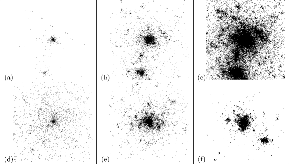
Figure 1: Illustrative examples of model realizations for different iterations $i$ and different exponents $\gamma$. (a-c) Different iterations of the model $i=6,10,14$ ($\gamma=2.5$, $N=630$). Growth takes place close to occupied sites. (d-f) Realizations with different exponents $\gamma=2.0,2.5,3.0$ (the occupation probability is $p\approx 0.04$, $N=630$). The smaller $\gamma$, the more scattered are the emerging structures, the larger $\gamma$, the more compact are they.

III Analysis

The model output depends on a set of factors. Beyond the exponent $\gamma$, the system size $N\times N$ needs to be chosen. As the model works iteratively, the emerging structures can be investigated at different iterations $i$. Moreover, we run the model for $M$ realizations in order to obtain better statistics.

Figure 1 shows examples of model realizations. Visually, the emerging structures could be associated with urban space. Figure 1(a-c) shows three iterations of a single realization. For high values of $\gamma$ the spatio-temporal evolution is strongly influenced by the sites which are occupied early, see Figure 1(d-f). Such a path dependency is also reflected in the reduction of rotational symmetry observed for increasing values of $\gamma$. In particular, the larger $\gamma$ is chosen, the more compact and less scattered are the obtained structures. Large $\gamma$ also leads to slower filling of the lattice.

III.1 Cluster size distribution

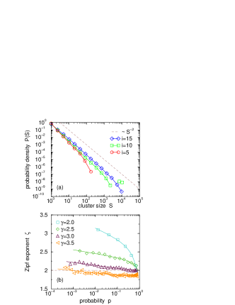
Figure 2: (Color online) Cluster size distribution and dependence of the Zipf exponent on the occupation probability. (a) Examples of probability density distributions $P(S)$ of the cluster size $S$ disregarding the largest cluster of each realization: $i=5,10,15$ (from top to bottom, $p\approx 0.004,0.078,0.573$), $\gamma=2.5$, $N=630$, $M=100$ (solid lines connect symbols). The two green dotted squares represent the contribution of the largest cluster ($i=10$). (b) The obtained Zipf exponents $\zeta$ as a function of the occupation probability $p$: $\gamma=2,2.5,3,3.5$ (from top to bottom), $N=630$, $M=100$. Solid lines are fits according to Eq. (3). Dashed lines indicate $\zeta=2$.

We begin our analysis by studying the cluster size distribution. We employ the City Clustering Algorithm (CCA) Rozenfeld et al. (2008, 2011) and find that the largest cluster is markedly larger than the remaining ones (Fig. 2(a)), i.e. larger than expected from Zipf’s law. The presence of such anomalous extremes in size distributions are denoted as Dragon Kings and are signatures of strongly cooperative dynamics Pisarenko and Sornette (2011). A similar effect has been found in another model Schweitzer and Steinbrink (1998), where – in order to avoid their appearance – the domination of the largest cluster is inhibited by excluding it from proportionate growth. Exclusion is not feasible in our model and we omit it when studying the cluster size distribution Makse et al. (1995, 1998).

Figure 2(a) shows examples of the probability density $P(S)$ of the cluster size $S$ disregarding the largest cluster of each realization. We find approximate power-laws according to

$$P(S)\sim S^{-\zeta}\,,$$ (2)

where $\zeta$ is the Zipf exponent. In Fig. 2(a) one can see, deviations from Eq. (2), in the form of too few large clusters. Naturally, for late iterations Eq. (2) extends over more decades of cluster size than for early iterations. As can be seen, the Zipf exponent is close to $2$. To be more precise, $\zeta$ is smaller for large iteration $i$ than for small $i$. Accepting minor deviations from $\zeta=2$, the model produces cluster size distributions compatible with Zipf’s law.

In order to better understand how $\zeta$ relates to the model parameters, we express the iteration $i$ in terms of the overall occupation probability $p$ which for a given $i$ is defined by the number of occupied sites divided by the total number of sites, i.e. $N\times N$. The probability $p$ increases monotonically with the iteration $i$. In Fig. 2(b) $\zeta$ is plotted as a function of $p$. As can be seen, it decreases monotonically with increasing probability and strongly depends on the model exponent $\gamma$. While for $\gamma<3$, convex $\zeta(p)$ are found with overall $\zeta>2$, for $\gamma=3$, an almost logarithmic form can be identified with $\zeta>2$ and $\zeta\rightarrow 2$ for $p\rightarrow 1$. In contrast, for $\gamma>3$, we see a slightly concave relation and $\zeta<2$ (except for small $p$). Accordingly, the Zipf exponent depends strongly on both, the model exponent $\gamma$ and the iteration of the model $i$.

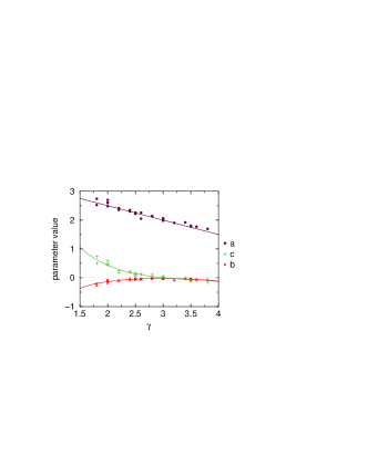
Figure 3: (Color online) Parameter values $a,b,c$ as a function of the exponent $\gamma$ from fitting the Zipf exponent versus the occupation probability (Fig. 2(b)). The dots represent the parameters obtained from fitting Eq.(3) to the numerical values, the solid lines are given by $a=-k_{1}\gamma+k_{2}$, $b_{\gamma\leq 3}=-{\rm e}^{-k_{3}\gamma+k_{4}}$ and $b_{\gamma>3}=-{\rm e}^{k_{3}\gamma-k_{5}}$, and $c={\rm e}^{-k_{6}\gamma+k_{7}}-{\rm e}^{-k_{8}+k_{7}}$ ($k_{1}$-$k_{8}$ are fitting parameters). In order to have enough values, we do not separate the different system sizes.

Moreover, we find that the dependence of $\zeta$ on $p$ can be well approximated by

$$\zeta(p)=a+b\ln(p)+c\ln(1-p)\,,$$ (3)

which also is the logarithm of a beta-distribution. The solid lines in Fig. 2(b) are non-linear fits to the numerical model results, providing the fit parameters $a$, $b$, and $c$. In Fig. 3 the obtained values of these parameters are plotted against $\gamma$.

III.2 Fractality

Next we analyze fractal properties of the urban envelope of the largest cluster. Therefore, we first extract the boundary of the cluster. This is done, by identifying those largest cluster sites which have at least one empty neighboring cell which connects to the system border via a nearest neighbor path of empty sites (the latter condition is necessary to exclude inclusions). Thus, here the boundary is defined as the occupied neighbors of the external perimeter Grossman and Aharony (1987). Then we apply box-counting, i.e. perform coarse-graining and count how many sites or occupied. Thus, we regularly group $m\times m$ sites and accordingly reduce the system size to $(N\times N)/(m\times m)$. Finally, we count the number of occupied sites $N_{\text{B}}$ for a chosen box size $m$.

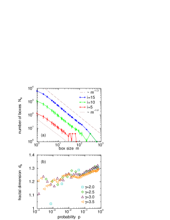
Figure 4: (Color online) Self-similar scaling of the boundary of the largest cluster. (a) Number of boxes necessary to cover the boundary as a function of the size of the boxes: $\gamma=2.5$, $N=630$, $i=5,10,15$ ($p\approx 0.004,0.078,0.573$), $M=100$. The results follow Eq. (4) indicating the fractal property of the boundary with a fractal dimension $1<d_{\text{B}}<2$. The error bars represent standard deviations among the realizations. (b) Fractal dimension as function of the occupation probability for $\gamma=2.0,2.5,3.0,3.5$ ($N=630$, $M=100$). $d_{\text{B}}$ increases approximately logarithmically, independent of $\gamma$.

Examples of $N_{\text{B}}(m)$ are displayed in Fig. 4(a). Apart from minor deviations for small and large $m$, straight lines are found in the log-log representation, corresponding to

$$N_{\text{B}}(m)\sim m^{-d_{\text{B}}}\,,$$ (4)

where $d_{\text{B}}$ is a measure of the fractal dimension of the cluster boundary. In the displayed examples, we approximately find $d_{\text{B}}\approx 1.25$.

Figure 4(b) shows $d_{\text{B}}$ as a function of the occupation probability $p$. Qualitatively, we find a logarithmic dependence, implying $d_{\text{B}}\rightarrow\text{const.}$ for $p\rightarrow 1$, which seems to be independent of $\gamma$. Overall, the values are clearly below those expected from uncorrelated percolation slightly above or below the percolation transition Voss (1984). This difference could be due to inherent correlations in our model. Nevertheless, the model generates self-similar (fractal) largest clusters. The evolving fractal dimension is at least qualitatively consistent with urban areas, see e.g. Shen (2002).

Last, we would like to note that the definition of the boundary has a substantial influence on the fractal dimension Grossman and Aharony (1987). Moreover, box-counting results can differ from those obtained with other techniques such as the equipaced polygon method Kaye and Clark (1985). Further analysis is required to shed light on these aspects.

III.3 Percolation transition

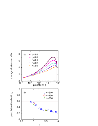
Figure 5: (Color online) Percolation transition of the model. (a) Average size of the finite clusters: $\gamma=3.8,3.6,3.4,3.2,3.0$ (from top to bottom), $N=210$, $M=1000$. The vertical line represents the percolation transition of uncorrelated percolation $p^{*}_{\text{c}}\simeq 0.593$ (site percolation in the square lattice, Bunde and Havlin (1991)). The maximum is located at the percolation transition. (b) Percolation transition $p_{\text{c}}$ as a function of $\gamma$: $N=210,420,630$ ($M=1000,400,100$). For small $\gamma$ the percolation transition is close to $p^{*}_{\text{c}}$ as indicated by the horizontal line.

One may argue that at certain iteration the system might undergo a percolation transition. Thus, finally we characterize the percolation threshold of the model. Therefore, we calculate the average cluster size disregarding the largest component, $\langle S\rangle$, as a function of the occupation probability $p$. At the percolation transition, $p_{\text{c}}$, the average cluster size exhibits a maximum Bunde and Havlin (1991). Figure 5 depicts $\langle S\rangle(p)$ for some values of $\gamma$. A distinct peak can be found which moves to larger $p$ with decreasing $\gamma$. For $\gamma<3$ the maximum becomes less clear and we cannot determine $p_{\text{c}}$.

The obtained percolation thresholds are plotted versus $\gamma$ in Figure 5(b). The transition decreases monotonically with increasing $\gamma$. For $\gamma\approx 3$ the value is close to the transition of uncorrelated site percolation in the square lattice ($p^{*}_{\text{c}}\approx 0.593$, Bunde and Havlin (1991)). For $\gamma\approx 4$ we find $p_{\text{c}}\approx 0.2$.

We would like to note that the results of Zipf and fractality analysis seem to be independent from percolation transition, i.e. there is no change in the behavior below or above $p_{\text{c}}$. Accordingly, scaling in the form of Zipf’s law and fractality are reproduced even away from criticality.

IV Analyzing real data

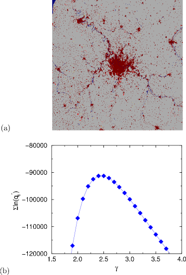
Figure 6: (Color online) Urban growth and the estimation of $\gamma$ for Paris and it’s surroundings in the years 2000 and 2006. (a) Considered land-cover data in a window of $1000\times 1000$ grid points ($250$ m resolution). The panel distinguishes the following sites: populated in 2000 (dark red), unpopulated in 2000 (grey), water (blue), non-urban $\rightarrow$ urban (light red), and urban $\rightarrow$ non-urban (yellow). (b) Log-likelihood of urbanization. First we calculate the probabilities $q_{j}$ according to Eq. (1) for the year 2000, whereas ($w_{k}=1$ for urban and $w_{k}=0$ for non-urban cells). Then we determine $Q$ according to Eq. (5) over all non-urban cells in 2000 (the change urban to non-urban is disregarded). We find a maximum at $\gamma_{\text{Paris}}\approx 2.5$.

Finally, it is of interest which $\gamma$-value real city growth exhibits. In order to address this question, we consider Paris and its surroundings. We analyze CORINE Bossard et al. (2000) land-cover data in $250$ m resolution and only distinguish between urban and non-urban land grid cells. For the years 2000 and 2006 we extract a window of $1000\times 1000$ grid points (Fig. 6(a)) and study the land-cover change. Since our model only includes growth, we focus on those cells which change from non-urban to urban and disregard the opposite.

First we calculate the probabilities $q_{j}$ according to Eq. (1) for the year 2000, with $w_{k}=1$ for urban and $w_{k}=0$ for non-urban cells. Then we determine the log-likelihood by summing over all non-urban cells in 2000,

$$Q=\sum_{j\in A}\ln q_{j}+\sum_{j\in B}\ln(1-q_{j})\,,$$ (5)

where $A$ is the set of cells changing from non-urban to urban and $B$ is the set of cells remaining non-urban. Varying $\gamma$ we can identify the value for which $Q$ is maximized, i.e. for which the probabilities calculated with Eq. (1) best represent the non-urban to urban land-cover change in the real data. As can be seen in Fig. 6(b), the maximum is located at $\gamma_{\text{Paris}}\approx 2.5$. The qualitative similarity between Fig. 6(a) and Fig. 1(e) supports this quantitative result, but the comparison also shows that the real example is richer in structure. While the analysis does not provide sufficient evidence to support our model, it leads to the value of $\gamma$ for which the model best fits the growth of Paris.

V Discussion

We also find that the growth rate of clusters between two iterations is independent of the cluster size (not shown). This implies proportionate growth, a characteristic which is also featured by preferential attachment Simon (1955); Barabási and Albert (1999). We would like to note that in the proposed model such mechanism emerges and is not included explicitely. We further find that the standard deviation of the growth rate decays as a power-law with exponent $1/2$ (not shown) which indicates uncorrelated growth Rozenfeld et al. (2008); Rybski et al. (2009). Again, analyzing the growth, we have disregarded the largest cluster.

While the work in hand briefly introduces our model, more research is necessary to characterize it. This includes (i) an analytical description of the model, (ii) further numerical analysis, in particular refining the fractal characterization (as mentioned in Sec. III.2) or other features such as the area-perimeter scaling Andersson et al. (2002), and (iii) relating our model to other physical approaches, such as Andersson et al. (2002); Jeon and McCoy (2005); Ree (2006).

The analogy of gravitation has a long history in geography and spatial economy. However, the early works were limited by scientific background from statistical physics as well as computational power. Here we reexamine the concept of gravity cities by proposing a simple statistical model which generates city-like structures. The emergent complex structures are similar to urban space. On the one hand, we find that the largest cluster which can be considered as Central Business District Makse et al. (1995) exhibits fractality, consistent with measured urban area. On the other hand, clusters around the largest one can be considered as towns surrounding a large city Makse et al. (1995). Their cluster size distribution is compatible with Zipf’s law.