A new method to detect solar-like oscillations at very low S/N using statistical significance testing

Abstract

We introduce a new method to detect solar-like oscillations in frequency power spectra of stellar observations, under conditions of very low signal to noise. The Moving-Windowed-Power-Search, or MWPS, searches the power spectrum for signatures of excess power, over and above slowly varying (in frequency) background contributions from stellar granulation and shot or instrumental noise. We adopt a false-alarm approach (Chaplin et al. 2011) to ascertain whether flagged excess power, which is consistent with the excess expected from solar-like oscillations, is hard to explain by chance alone (and hence a candidate detection).

We apply the method to solar photometry data, whose quality was systematically degraded to test the performance of the MWPS at low signal-to-noise ratios. We also compare the performance of the MWPS against the frequently applied power-spectrum-of-power-spectrum (PS$\otimes$PS) detection method. The MWPS is found to outperform the PS$\otimes$PS method.

1 Introduction

Asteroseismology on solar-like oscillators can provide important knowledge on the internal structure and evolution of these stars, and in the case of planetary systems this knowledge is needed for much of the analysis on the planets themselves. The analysis and interpretation of the stellar oscillations relies of course on the actual detection of the signatures of the solar-like oscillations. These signatures manifest as a pattern of near regularly spaced peaks, and hence a power excess, in the frequency spectrum of the stellar time series. The advent of space-based photometric observations, such as those provided by the NASA Kepler Mission (Borucki et al. 2010; Koch et al. 2010), is providing large quantities of exquisite-quality data for asteroseismology (Gilliland et al. 2010). The first stage of asteroseismic analysis of solar-type stars often now involves the application of automated analysis pipelines to search for signatures of stellar oscillations. These signatures may then be analysed in detail if a positive detection is obtained.

Many of the methods exploit the near regularity (or periodicity) in frequency of the oscillation frequencies, for example from computation of the autocorrelation of the timeseries (equivalently the power spectrum of the power spectrum, or PS$\otimes$PS) (see, e.g., Hekker et al. 2010; Mosser & Appourchaux 2009), or the autocorrelation of the power spectrum (see, e.g., Campante et al. 2010; Karoff et al. 2010) and variants thereof (see, e.g., Verner & Roxburgh 2011; Huber et al. 2009; Mathur et al. 2010). These methods will have difficulty in detecting a signal if the regular structure is obscured, as for example in stars with many mixed-modes, or in stars where the stellar oscillation signal is buried in noise so that beating with the noise becomes significant.

Here, we present a method that instead searches just for the power excess originating from stellar oscillations. This Moving-Windowed-Power-Search method (hereafter MWPS) uses a moving window in frequency, and a statistical significance test is employed to see if any excess power flagged over and above the expected sources of background noise could be caused solely by fluctuations of the noise. The method does not rely on detecting any regular frequency structure in the stellar oscillation spectrum and is shown to work extremely well under low signal to noise (low SNR) conditions. To see how the MWPS method performs compared to currently used methods, we test it against the PS$\otimes$PS method, which is one of the most commonly used techniques for extracting the large frequency separation. Both methods are tested on solar data, to which increasing amounts of white noise were added in the time series.

The layout of the rest of the paper is as follows. In Section 2 we introduce the principles of the MWPS method, and discuss in detail its implementation. The PS$\otimes$PS, with which we compare the MWPS, is discussed in Section 3. We present results of testing both methods on solar data in Section 4. Concluding remarks are given in Section 5.

2 Moving-Windowed-Power-Search

2.1 Overview

The oscillation spectrum of a solar-type star consists of a series of regularly spaced peaks with heights modulated by a broad envelope. This envelope of power due to oscillations may be approximated by a Gaussian, with $\nu_{\rm max}$ defined as the frequency at the peak of the power envelope of the oscillations where the observed modes present their strongest amplitudes (Chaplin et al. 2011).

The power due to the oscillations sits on a slowly varying (in frequency) background power that we assume is dominated by contributions from shot/instrumental noise, stellar granulation and activity. When the observed power in the oscillations relative to the background is high (i.e., high SNR), the power excess due to the oscillations will be clearly visible. However, at low SNR, statistical fluctuations in the background power may swamp the oscillations signal, so that the excess is much harder to see.

The MWPS method searches the spectrum for the presence of excess power, over and above the slowly varying background. A statistical false-alarm (null hypothesis) test is applied to ascertain whether any flagged excess is hard to explain by chance alone, i.e., random fluctuations of the background. Such cases may be flagged as candidate detections, subject to some a priori constraints regarding the total excess power solar-like oscillations would be expected to show in the flagged frequency range (of which more in Section 2.3 below).

The method is clearly reliant on providing an accurate estimate of the underlying background, since any excess is defined relative to that background. The background fitting is discussed in detail below, in Section 2.4. First, we discuss the statistics of the MWPS (Section 2.2), and logistics relating to how the frequencies are searched for evidence of a power excess (Section 2.3).

2.2 Statistics of the MWPS

At each tested frequency we estimate a power-to-background ratio, $\text{PBR}_{\rm tot}$, over a pre-defined window in frequency. This ratio is defined according to

$$\rm PBR_{\rm tot}=\frac{P_{\rm tot}}{B_{\rm tot}},$$ (1)

where $\text{P}_{\rm tot}$ is the total power across the test frequency window, i.e., it includes any excess power above the underlying fitted background, and the contribution from the background; and $\text{B}_{\rm tot}$ is the total power in the background, i.e., the area below the fitted background curve. Note that this definition of PBR_tot corresponds to the value of SNR_tot+1 in Chaplin et al. 2011. The value of $\text{PBR}_{\rm tot}$ is normalised in such a way that it will tend to $\text{PBR}_{\rm tot}\sim 1$ in the case of no excess power from oscillations. The motivation for using a window instead of simply the entire power spectrum is, that by using a frequency range much larger than the one containing the excess power from oscillatons, the value of $\rm PBR_{\rm tot}$ would be much degraded, reducing the chances of making a detection. The tested frequencies and associated window widths are discussed in Section 2.3 below.

We assume that the individual bins of the power spectrum follow $\chi^{2}_{2}$ statistics, i.e. that they follow a chi-squared distribution with two degrees-of-freedom (d.o.f.). As the sum of two such independent distributions $\chi^{2}_{k}+\chi^{2}_{m}$ is yet another $\chi^{2}_{n}$ distribution with $n=k+m$ d.o.f., the sum of power from the $N$ independent bins included in the envelope interval will then be distributed according to a $\chi^{2}$ distribution with $2N$-d.o.f. We may therefore compare the value of $\text{PBR}_{\rm tot}$ with a $\chi^{2}$ 2$N$-d.o.f. statistic (Appourchaux et al. 2004). The functional form of the $\chi^{2}$ distribution is given by:

$$f(x;k)=\frac{1}{2^{k/2}\Gamma(k/2)}x^{k/2-1}e^{-x/2},$$ (2)

where $k$ is the number of d.o.f., $\Gamma$ is the gamma function and $x$ is the calculated value of $\text{PBR}_{\rm tot}$ (actually $x=\text{PBR}_{\rm tot}k$).

Knowing the distribution, it is possible to calculate a corresponding probability, or $p_{\rm value}$, for the obtained value of $\text{PBR}_{\rm tot}$, i.e. the probability of observing a value $\geq x$ by chance, assuming the null hypothesis is true, i.e.,

$$p_{\rm value} =1-F(x;k)$$ (3)

$$=1-\int_{x}^{\infty}f(x;k)dx$$

where $F(x;k)$ is the cumulative $\chi^{2}_{k}$ distribution. Needless to say, the lower the $p_{\rm value}$ the less likely it is that the observed power can be attributed to random fluctuations of the underlying background. If the $p_{\rm value}$ falls below a pre-defined significance level (or false alarm probability), $\alpha$, the null hypothesis can be rejected and the observed power is then assumed to be statistically significant. Here, we have set $\alpha=0.01$.

The threshold value of $\text{PBR}_{\rm tot}$ required to reject the null hypothesis is given by:

$$P(\rm PBR_{\rm tot}\geq\rm PBR_{\rm threshold})=\alpha,$$ (4)

which amounts to finding the PBR at which $p_{\rm value}=\alpha$. In sum, the ”false-alarm” approach means that every calculated $p_{\rm value}$ falling below $\alpha$ is flagged as marking the presence of significant excess power, which could be attributable to stellar oscillations. The procedure thereby gives us a probability curve across the frequency interval for each of the selected windows.

2.3 Tested frequencies and window widths

We make no a priori assumptions on the true value of $\nu_{\rm max}$ and thereby on the range of frequencies covered by any Gaussian power envelope that might be present. However, we do allow for the fact that the FWHM in frequency of the oscillation envelope is known to vary to good approximation as $\nu_{\rm max}/2$ (see, e.g., Stello et al. 2007; Chaplin et al. 2011), and so test for the presence of excess power over windows of the spectrum whose width in frequency is varied accordingly.

The centre frequency of each test window may be regarded as a proxy for $\nu_{\rm max}$. When the MWPS is applied at low frequencies the width of the test window should be set fairly narrow, since any oscillation signal present will also be confined over a narrow range of frequencies. A wide test window – i.e., one significantly wider than the oscillation power envelope – would reduce the underlying PBR, and hence reduce the chances of making a detection with the MWPS. The same logic dictates that the window width must be set much wider when the test is applied at higher frequencies (too narrow a window will result in signal being missed).

Assuming a Gaussian-like power excess, there is notionally an optimum window width that will maximize the underlying PBR, which corresponds approximately to $1.17$-times the FWHM of the power envelope, which is $0.59\times\nu_{\rm max}$, i.e., $0.59$-times the test frequency. This width may not always yield optimum results in practice, due to the importance at low SNR of beating with background noise, and the impact of realization noise from any oscillations that are present. We make suitable allowance for this in our adopted search strategy.

We begin by selecting 40 frequencies spread evenly in the range from 1000 to $5000\,\rm\mu Hz$ (adopted range for solar-like oscillations). An optimum window width is calculated for each of these $\nu_{\rm max}$ proxy frequencies, giving a total of 40 windows with which to test the power spectrum. Each window is then moved through the power spectrum in steps set by a pre-defined lag frequency (overlaps, but not gaps, between frequency ranges encompassed by the respective windows are allowed), and the MWPS test is applied at each location. The check for excess power at each location involves first calculating the total power in the envelope interval set by the window width, which may then be compared to the total power found below the fitted background (see Section 2.4 below for details of the background fitting).

We do not vary the window size as each window is moved through the spectrum. The reason for this is twofold: First, it turns out that varying the window width tends to skew the resulting SNR and $1/p_{\rm value}$ curves, mainly due to overlap effects as the window grows in size towards higher frequencies, and this inevitably introduces an unwanted offset in the peak position of the detectability, i.e., in the estimated $\nu_{\rm max}$. Second, use of a single varying window does not take into account that the selected (notionally optimal) window size may not be optimal in practice, as noted above.

Application of the MWPS as outlined above yields an SNR (or equivalently PBR) curve and a corresponding $1/p_{\rm value}$ curve, as a function of frequency for each of the adopted 40 window widths. An ensemble analysis of those curves which have values of $1/p_{\rm value}$ that exceed the detection threshold then yields an estimate of $\nu_{\rm max}$. We discuss this procedure in detail in Section 4 below.

We then apply a sanity check on the results. The total power in the oscillations spectrum is a strong function of $\nu_{\rm max}$, i.e., the higher $\nu_{\rm max}$, the smaller is the expected total oscillations power. We apply the following formulae from Chaplin et al. (2011) to estimate the expected total power, based on the estimated $\nu_{\rm max}$:

$$\rm P_{tot}\approx 1.55A_{max}^{2}\eta^{2}\frac{\nu_{max}}{\Delta\nu}$$ (5)

$$\eta^{2}=sinc\left[\pi/2\left(\frac{\nu_{\rm max}}{\nu_{Ny}}\right)\right]$$ (6)

Here $\rm P_{tot}$ is the total power underneath the Gaussian shaped envelope in the range $\pm\rm\nu_{max}/2$ around the estimated $\nu_{\rm max}$ value, and $\rm A_{max}$ is the radial-mode amplitude at $\nu_{\rm max}$. The factor $\eta^{2}$ is a correction for the apodization of the oscillation signal the closer $\nu_{\rm max}$ is to the Nyquist frequency, $\nu_{Ny}$, and $\Delta\nu$ is the average large separation (see discription to Eq. 10) which may be estimated from $\nu_{\rm max}$ (see Eq. 14). This prediction may then be compared to the measured excess power in the spectrum. If the measured excess is significantly higher than the predicted excess (i.e., by some multiple of the combined uncertainties on the prediction and measurement) the candidate detection is flagged as questionable. Strong, narrow-band artefacts can produce signatures of this type, hence knowledge of known instrumental issues is important to help try to verify the robustness (or otherwise) of any claimed detection.

2.4 Fitting the background

Since the success of the MWPS method relies heavily on a good fit of the background, we devote this section to a description of the background fitting process.

We took the approach of a $\chi^{2}$-minimization instead of directly maximising the likelihood function of the power spectrum (having a $\chi^{2}_{2}$-statistic) mainly to decrease the computation time for the fitting. In order to use a $\chi^{2}$ procedure the power spectrum is binned linearly in $\text{ln}(\rm\nu)$. This ensures first of all that the points used in the background fit are independent and secondly, that the density of points in frequency is larger towards lower frequencies where the bulk of variations due to background phenomena occur. The averaged datum with the smallest number of binned frequencies used in the fitting tests (Section 4) came from an average made over $\sim 550$ frequency bins, which makes it safe to assume that the points will have a normal distribution, justifying the use of a $\chi^{2}$-minimisation scheme:

$$\chi^{2} =\sum_{i=1}^{N}\left[\frac{y_{i}-bg(x_{i};\textbf{a})}{\sigma_{i}}\right]^{2},$$ (7)

$$\sigma_{i} =\frac{bg(x_{i};\textbf{a})}{\sqrt{n}}.$$ (8)

Here the sum is over the binned data, $y_{i}$ is the value of the binned datum $i$. $bg(x_{i};\textbf{a})$ is the value of the fitted background function, where a are the dependent variables for the background function. The weighting, given by $\sigma_{i}$, depends as seen on the number of frequencies, $n$, included in the binning.

The function describing the background signal consists of power laws (Harvey 1985), each of which describes a specific physical phenomenon. The power laws included describe the signal due to, respectively, stellar activity and granulation, given by (see, e.g., Hekker et al. 2010; Mathur et al. 2011):

$$bg(x_{i};\textbf{a})=\frac{A_{g}}{1+(B_{g}x_{i})^{c}}+\frac{A_{a}}{1+(B_{a}x_{i})^{2}}+S_{N}.$$ (9)

In this equation $A_{g}$ and $A_{a}$ give the power of granulation and activity respectively, while $B_{g}$ and $B_{a}$ represent the characteristic time scales for the two phenomena as the power remains approximately constant on time scales longer than $B_{g/a}$ (or equivalently frequencies lower than $B_{g/a}^{-1}$), and drops off for shorter time scales. In the fitting, the exponent, $c$, of the granulation slope is kept as a free parameter, while the exponent for the activity slope is fixed to a value of 2. The fixed value of 2 for the slope of the activity component arises from the fact that we assume an exponential decay of the activity regions as a function of time. The constant parameter $S_{N}$ gives the photon shot noise. Whilst the method was tested we omitted binned data from the first $250\rm\ \mu Hz$ of the power spectrum, so that only the granulation and the shot noise was needed to fit the background. The reason for only including these two components is that phenomena related to activity, such as e.g. spots (both intrinsic variations and rotational modulation), mesogranulation and supergranulation all have characteristic time scales longer than $4000$ s (see, e.g., Harvey 1985), equivalent to frequencies below $250\rm\ \mu Hz$.

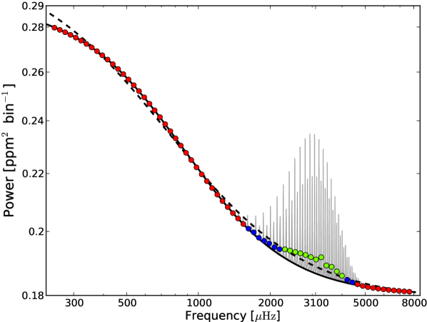
Figure 1: Illustration of the impact of applying the runs-test, here shown on artificial noiseless data shown as the limit power spectrum in grey. This limit spectrum is modelled as a series of Lorentzian peaks with a regular frequency spacing and a height modulated by a Gaussian envelope (see Eq. 10), which sits on top of a slowly varying background function. The points in the figure are the values for the binned spectrum. The dashed black curve shows the background fit to all the binned points, and as seen the fit is somewhat offset from the expected level. The green points mark the longest consecutive series of points above the background curve. The solid black curve gives the best fit to the red points, i.e., after removing the points flagged by the runs-test (green) along with the additional points on either side, given by the blue points.

A general problem when fitting the background to the power spectrum is of course that any excess power from stellar oscillations will offset the background fit, primarily through an overestimated value of the constant shot noise component, and make it very difficult to pin down the correct value for the slope of the background function (see Fig. 1) which again could produce unwanted peaks in the calculated SNR curves. As this offset will lower the PBR value it can have a determining impact on the performance of the MWPS method, especially in high noise cases.

To boost the robustness of our method and circumvent the offset from a potential power excess, a Wald-Wolfowitz runs-test (see Barlow 1989) is applied to the intial background fit to check for non-random offsets around the fitted curve. This type of information in not obtainable from the fitting procedure as the $\chi^{2}$-minimization is, by its very nature, completely blind to the sign of any deviation, whereas the Wald-Wolfowitz runs-test is blind to anything but the sign of the offset making it a good complimentary test. Any power excess which is strong enough to offset the background fit will be distributed in such a way that there will be a relatively long run (i.e., a consecutive series) of points above the fitted curve at the position of the power excess (see Fig. 1). If the false-alarm probability obtained from the runs-test falls below a given value – indicating that the chances of the run occuring by chance are low – it may be assumed that the background fit is offset due to some power excess not described by the background function.

The points comprising the longest consecutive series above (in power) the background fit are removed in addition to a certain user defined number of points at the low- and high-frequency ends of this series, and the background is fitted anew to the remaining binned points. In our testing we generally removed seven additional points at the low-frequency end, and three at the high-frequency end (remember that as the binned points are linear in $\text{ln}(\rm\nu)$ the distance in frequency between two points at the low-frequency end is much shorter than the equivalent distance at the high-frequency end).

If the best-fitting $\chi^{2}$-value remains high after this procedure has been applied, an extra power law could potentially be included in the background fit until a satisfactory fit is obtained. A good fit corresponds to a reduced $\chi^{2}$-value of $\chi^{2}_{r}\sim 1$. If the reduced $\chi^{2}$-value is lowered after the removal of the longest run from the runs-test, the MWPS procedure continues, even if this removal of points worsens the result from the runs-test. In this sense the probabilities from the runs-test are used more as indicators of a good fit, while the configuration of runs is actively used.

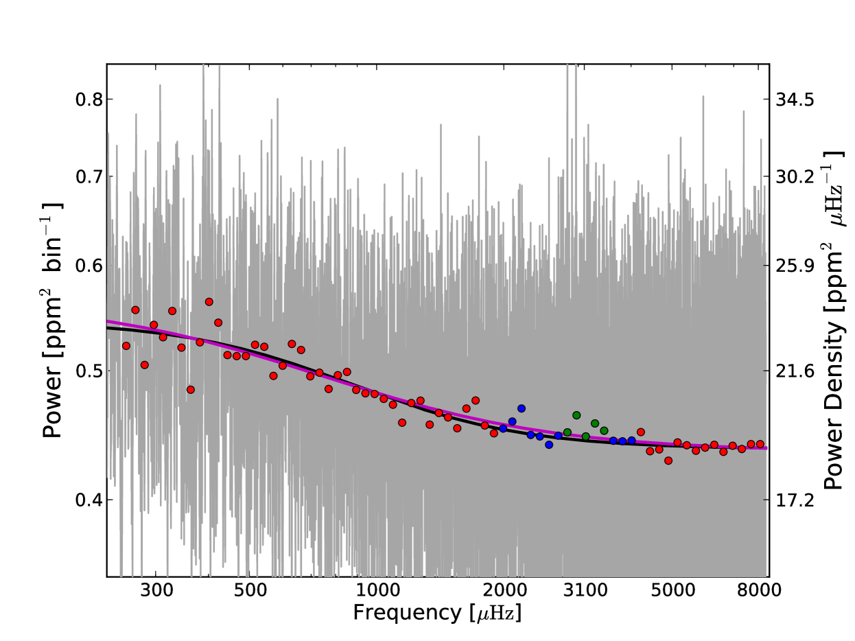
Figure 2: Example background fit for one of the $\sigma=280$ ppm realizations. The $1\rm\ \mu Hz$ smoothed power spectrum is plotted in gray, from 230 to $8500\rm\ \mu Hz$. The red points show the binned power spectrum. The longest run found by the runs-test is shown with the green points, and the additional points to be removed are plotted in blue. Also shown is the fitted background function before (magenta) and after the exclusion of the green and blue points (black).

We employed a Nelder-Mead simplex algorithm for the minimisation of the $\chi^{2}$-value, as this seems to perform in a very robust manner albeit at the expense of being somewhat slower than other frequently applied methods, e.g. steepest descent methods.

The starting values of the parameters of the background model were found as follows: For the granulation parameters – i.e., the granulation time scale $B_{g}$ and amplitude $A_{g}$ – we use information from the first derivative of the binned power spectrum in logarithmic units. This derivative is found by applying a third-order Savitzky-Golay (Savitzky & Golay 1964) smoothing filter to the binned power spectrum, from which the first derivative is directly obtainable. For the Savitzky-Golay filter we chose a window width of 41 points. In a first derivative curve like the one found, peaks will correspond to a rise or fall (i.e., a change) in power spectral density as a function of frequency. As mentioned in connection to Eq. 9, the contribution from granulation in the power spectrum falls at frequencies above $B_{g}^{-1}$. The granulation time scale is expected to be shorter than the equivalent time scale for the activity and so we identify the highest frequency peak in the first derivative curve as originating from the change in power due to the granulation, from which one can readily find the associated time scale. For the amplitude $A_{g}$ we find, in the first derivative curve, the frequency of the first dip to the low-frequency side of the granulation timescale peak, and use the power spectral density in the power spectrum at this frequency as the estimate for $A_{g}$. The shot noise level is estimated from the mean power spectral density at the high-frequency end of the power spectrum. Even though the Nelder-Mead algorithm is intended for localised optimisation, we found no significant change in the resulting background fits when the starting values for the optimisation were varied slightly, which is to be expected given the low number of fitting parameters.

3 Comparison method

We have compared the MWPS method against the power-spectrum-of-power-spectrum, or PS$\otimes$PS, method. For solar-like oscillators the PS$\otimes$PS method works well because high-order p-modes follow to good approximation a regular, periodic pattern in frequency (Tassoul 1980), described by

$$\nu_{n,\ell}=\Delta\nu(n+\frac{1}{2}\ell+\epsilon)-\ell(\ell+1)D,$$ (10)

where $n$ is the radial order and $\ell$ is the angular degree. $\Delta\nu$ is the so-called large separation, corresponding to the spacing in frequency between consecutive radial overtones, $n$, having the same angular degree, $\ell$. $\epsilon$ is a constant that is sensitive largely to the surface layers, and $D$ depends upon the sound-speed gradient in the deep interior of the star.

A near-regular pattern of modes in the power spectrum will produce significant peaks in the PS$\otimes$PS at locations corresponding to the prominent frequency separations. The most and next-most significant peaks are usually those corresponding to the separations $\Delta\nu/2$ and $\Delta\nu/4$, respectively (the former corresponding to the average separation between modes of odd and even degree, $\ell$). Before the PS$\otimes$PS is computed the power spectrum is first corrected for the background, by division of the best-fitting background model given by the procedure described in Section 2.4 above. The PS$\otimes$PS spectrum is then calculated from a window of the power spectrum centred on $\nu_{\rm max}$, as per the MWPS method. For our tests here we set the frequency window in power spectrum in advance, centered on the true location of $\nu_{\rm max}$ (rather than run a moving window through the spectrum).

The statistics of the individual and independent bins in the PS$\otimes$PS are also described to excellent approximation by $\chi^{2}$ 2-d.o.f. distribution. The probability of observing a relative power in a single bin greater than or equal to $s$ (i.e. the p-value, with $s$ the height divided by the background level of the PS$\otimes$PS) is just:

$$p(s)=\exp(-s).$$ (11)

We may then determine the probability of observing a single bin with a value of $s$ by chance out of $N$ bins of the PS$\otimes$PS by

$$P_{\rm chance}=[1-p(s)]^{\xi N},$$ (12)

where $\xi=1$ for a non-oversampled PS$\otimes$PS and $\xi\simeq 3$ for an oversampling by a factor of 10 (Chaplin et al. 2002). The final probability of observing a value greater than or equal to $s$ amongst $N$ bins in the PS$\otimes$PS spectrum (i.e., not by chance) is:

$$p_{\rm value}=1-[1-p(s)]^{\xi N}.$$ (13)

Again, if the value of $p_{\rm value}$ falls below $\alpha=0.01$ the case is flagged as a possible detection of stellar oscillations.

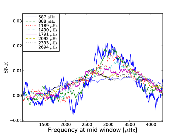
(a) SNR curves.

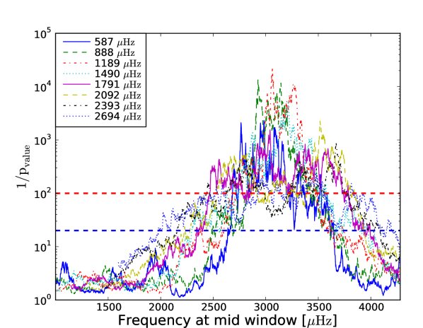
(b) $1/p_{\rm value}$ curves.

Figure 3: A typical result from an MWPS run, here for a realisation with $\sigma\leavevmode\nobreak\ =\leavevmode\nobreak\ 280$ ppm noise case. Panel (a) shows SNR curves for a representative sample of the 40 window widths (with widths indicated on the legend). Panel (b) shows the corresponding $1/p_{\rm value}$ curves. The red dashed line marks the one per cent significance level while the dashed blue line marks the five per cent significance level.

It is clear from Eq. 13 that the number of bins $N$ used in the computation is crucial in determining the absolute value of $p_{\rm value}$. Taking $N$ to be the total number of bins in the PS$\otimes$PS would only yield detections in very high SNR cases. However, we may use a priori knowledge on stellar oscillations to restrict the adopted value of $N$. The value of $\Delta\nu$ scales with $\nu_{\max}$ (Stello et al. 2009) according to

$$\Delta\nu=\alpha(\rm\nu_{max}/\mu Hz)^{\beta}$$ (14)

with values of $\alpha=0.22$ and $\beta=0.797$ (Huber et al. 2011). Predictions from stellar evolutionary models suggest that the value of $\Delta\nu$ given by the relation is accurate to around 15 per cent, which is the uncertainty we therefore adopt to define the search range around the $\Delta\nu/2$ value (having adopted the centre of the frequency window in the power spectrum as the proxy for $\nu_{\rm max}$). This decreases the value of $N$ significantly, compared to the total number of bins in the PS$\otimes$PS, and ensures that the method performs as effectively as possible when compared to the MWPS method.

4 MWPS and PS$\otimes$PS Tests

Both methods have been tested using a 500-day-long time series of photometric data on the Sun, obtained in the green band (500nm) of the VIRGO-SPM instrument (a full-disc Sun photometer) on board the ESA/NASA SOHO spacecraft. This time series has a duty cycle of nearly 99 per cent (Roca Cortès et al. 1999), which, combined with its long duration, makes it safe to assume independent frequency bins in the power spectrum with $\chi^{2}_{2}$ statistics. To this timeseries were added different levels of random Gaussian noise, with sample standard deviations covering the range $\sigma\leavevmode\nobreak\ =\leavevmode\nobreak\ \{180\ \text{ppm},200\ \text{ppm},\ldots,280\ \text{ppm}\}$, resulting in a total of six tested SNR levels. For each noise level we generated 20 power spectra, each having a different realization of the added random noise.

For all the power spectra we omitted the first $250\rm\ \mu Hz$ in the fit of the background, and found sufficiently good fits (in the sense of a low $\chi^{2}$-value) when including only the granulation and shot noise components. The chosen lag in frequency of the MWPS was $\sim 2.32\rm\ \mu Hz$ (equivalent to 100 frequency bins), which gives very good resolution. The bin size for the background binning was chosen as $\Delta_{\rm bin}=0.05$ (linear in $\text{ln}(\rm\nu)$). The envelope width of power excess was for all $\nu_{\rm max}$ proxies was taken to be $0.59$-times $\nu_{\rm max}$.

An example of one of the background fits is plotted in Fig. 2. It shows results on one of the realisations with $\sigma=280$ ppm. The plotted power spectrum has been smoothed with a $1\rm\ \mu Hz$-wide boxcar filter. The red points show the binned spectrum, to which the background function was fitted. The region with the longest run detected is shown by the green points, while the blue points show the additional points removed on the low- and high-frequency sides of the longest run. We also show the background fits to the points before (magenta curve) and after (black curve) the removal of the blue and green points. While the change in the background fit is quite subtle and hardly visible in this case, the reduced $\chi^{2}$ did change favourably, from a value of $\chi^{2}_{r}=1.24$ with 66 d.o.f. to $\chi^{2}_{r}=1.06$ with 51 d.o.f. Fig. 3 shows the MWPS results for the data plotted in Fig. 2. Panel (a) shows the SNR (i.e., $\rm PBR-1$) curves for several different window sizes (see plot anotation). The window sizes used here were selected as described in Section 2.3. A value of zero on the ordinate in effect corresponds to the total absence of oscillation signal. Negative values mean that the background was estimated to be higher than the actual observed power. Panel (b) shows the corresponding $1/p_{\rm value}$ curves. The dashed red line marks the one per cent significance level while the dashed blue line marks the five per cent significance level. Note that even though the most narrow window dominates the SNR curve its $1/p_{\rm value}$ is not as prominent due to the fact that its window comprises a smaller number of d.o.f. compared to the other windows.

We estimate $\nu_{\rm max}$ from the $1/p_{\rm value}$ curves as follows. We begin by calculating a mean $1/p_{\rm value}$ curve from all curves in which a detection was flagged. Using the mean curve instead of just the individual $1/p_{\rm value}$ curves ensures that if there are spurious peaks (e.g. from very narrow windows) these will not have a large impact as they are not seen in wider windows. The mean $1/p_{\rm value}$ curve is then smoothed with a Savitzky-Golay filter (which ensures that the area under the curve, the peak positions, and the width/height ratio of peaks, is conserved), with a window width of 61 points (corresponding to $\rm\sim 142\mu Hz$, with an adopted lag frequency of about $\rm 2.32\mu Hz$). The estimate of $\nu_{\rm max}$ is then given by the frequency at the highest value in this smoothed curve. To estimate the confidence limits on the estimated $\nu_{\rm max}$ we treat the smoothed, mean $1/p_{\rm value}$ curve as a probability density curve. Here the confidence limits are found by taking the 68.27$\%$ confidence intervals around $\nu_{\rm max}$ (see Barlow 1989). This is calculated by finding the shortest interval around $\nu_{\rm max}$ wherein 68.27$\%$ of the area under the curve is contained, equivalent to a one sigma limit for a Gaussian probability distribution. An example of an average $1/p_{\rm value}$ curve with estimated confidence limits can be seen in Fig. 4.

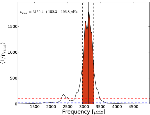
Figure 4: Smoothed average $1/p_{\rm value}$ curve, again for one of the $\sigma\leavevmode\nobreak\ =\leavevmode\nobreak\ 280$ ppm realizations. The solid black line gives the estimated $\nu_{\rm max}$, while the two dashed black lines represent the confidence interval (equivalent 1-$\sigma$ interval). The dashed red and blue lines correspond, respectively, to the one and five per cent significance levels.

For the computation of the significance in the PS$\otimes$PS we used the same background fits for correcting the power spectrum as were used for the MWPS method. For the search range, the adopted variation in the value of $\Delta\nu/2$ of $\pm 15$ per cent gave $N=13$ bins to be used in Eq. 13. The background level in the PS$\otimes$PS spectrum (not the power spectrum) was found by first smoothing the PS$\otimes$PS spectrum with a median filter. A low-order polynomial was then fitted to the smoothed spectrum, where the search range around $\Delta\nu/2$ was excluded from the fit. The PS$\otimes$PS was then divided by the fitted polynomial curve, giving relative power in the PS$\otimes$PS spectrum.

Fig. 5 shows non-oversampled and oversampled PS$\otimes$PS results for $\sigma=180$ and $\sigma=280$ ppm noise cases (the latter for the same data as Figs. 2, 3 and 4). The coloured regions in the figure show the range tested for significant power. Results are shown at both noise levels to illustrate the degradation of the PS$\otimes$PS signal in going from the lowest to the highest noise case considered. The $\sigma=280$ ppm signal may be compared with the firm detection found at this noise level by the MWPS method.

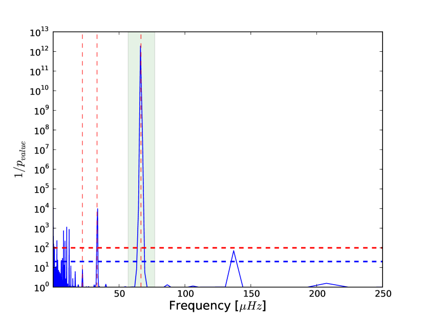
(a) Non-oversampled PS$\otimes$PS spectrum, $\sigma=180$ ppm noise.

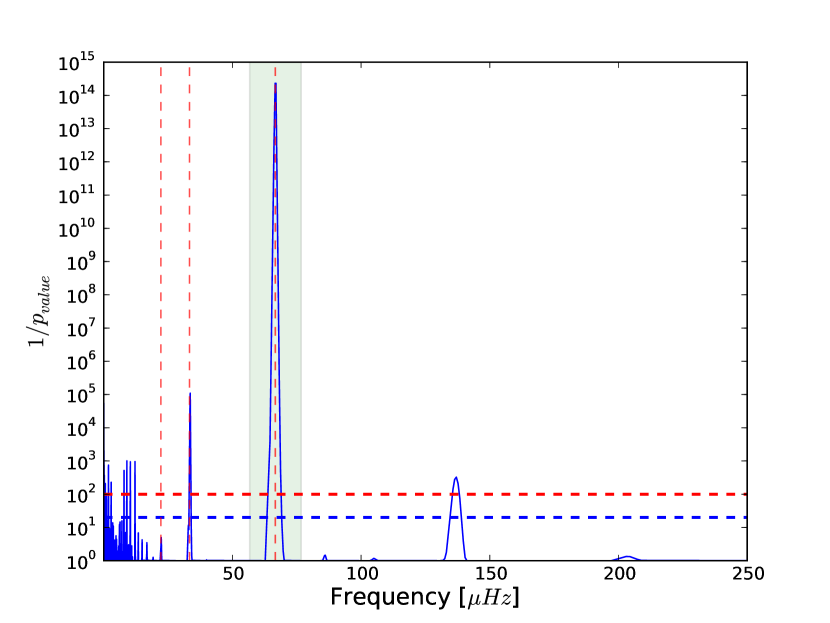
(b) PS$\otimes$PS spectrum oversampled by a factor of 10, $\sigma=180$ ppm noise.

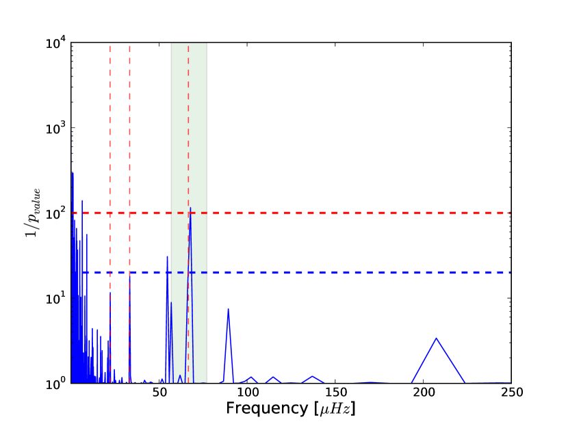
(c) Non-oversampled PS$\otimes$PS spectrum, $\sigma=280$ ppm noise.

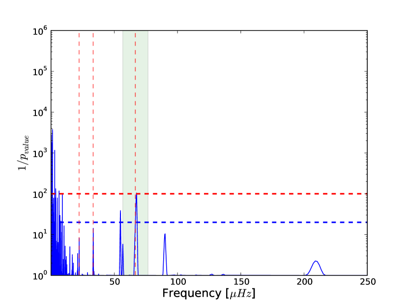
(d) PS$\otimes$PS spectrum oversampled by a factor of 10, $\sigma=280$ ppm noise.

Figure 5: Results of applying the PS$\otimes$PS method to one of the $\sigma=180$ and $\sigma=280$ ppm noise realizations. The spectra shown in this figure, each have a $1/p_{\rm value}$ that lies close to the median value for the respective noise levels, see Fig. 6. Panel (a): $1/p_{\rm value}$ for non-oversampled PS$\otimes$PS spectrum of the background corrected power spectrum. Here, the PS$\otimes$PS spectrum has been divided through by a smoothed background curve, and the $1/p_{\rm value}$ has been calculated using Eq. 13. The shaded area shows the $\pm 15$ per cent interval around $\Delta\nu/2$ which is used as the search range for significant power. Panel (b): oversampled result for the same dataset. Panels (c) and (d): results of applying the PS$\otimes$PS method to one of the $\sigma\leavevmode\nobreak\ =\leavevmode\nobreak\ 280$ ppm noise realizations (same data used to generate MWPS results in Fig. 3). The red and blue dashed lines mark the one per cent and five per cent significance levels respectively. The dashed vertical lines give the position, in frequency, of $\Delta\nu/2$, $\Delta\nu/4$, and $\Delta\nu/6$.

4.1 Results

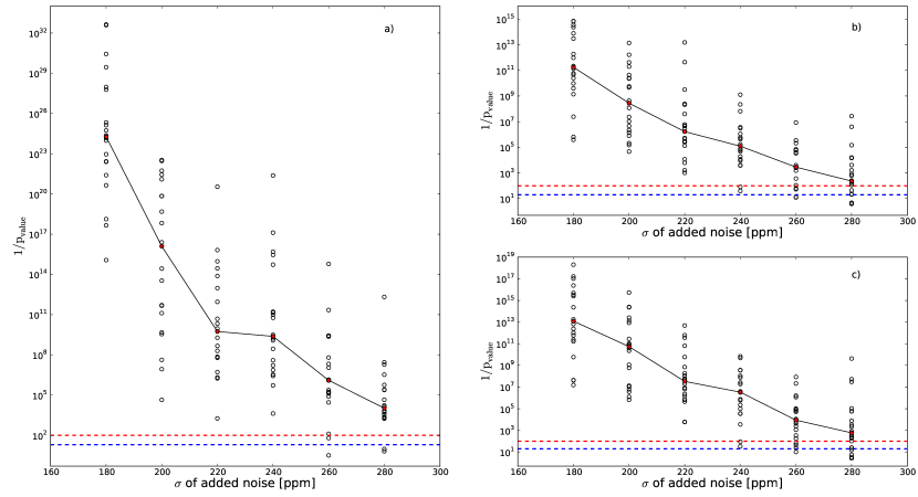
Figure 6: Results from the 20 different realisations of the $\sigma=180$ ppm to $\sigma=280$ ppm noise cases. Panel (a) shows the results obtained from the MWPS method, while panels (b) and (c) show the corresponding results from the PS$\otimes$PS method (no oversampling, and over-sampling by a factor of 10). The values in the MWPS plot, given by open symbols, are the maxima $1/p_{\rm value}$ of the smoothed, average $1/p_{\rm value}$ curves for the individual realisations. In all panels the open symbols show results of the individual realisations, while the red symbols are the median $1/p_{\rm value}$ value over all realisations at each noise level. The red and the blue dashed lines show the threshold values for, respectively, a one per cent and a five per cent detection threshold.

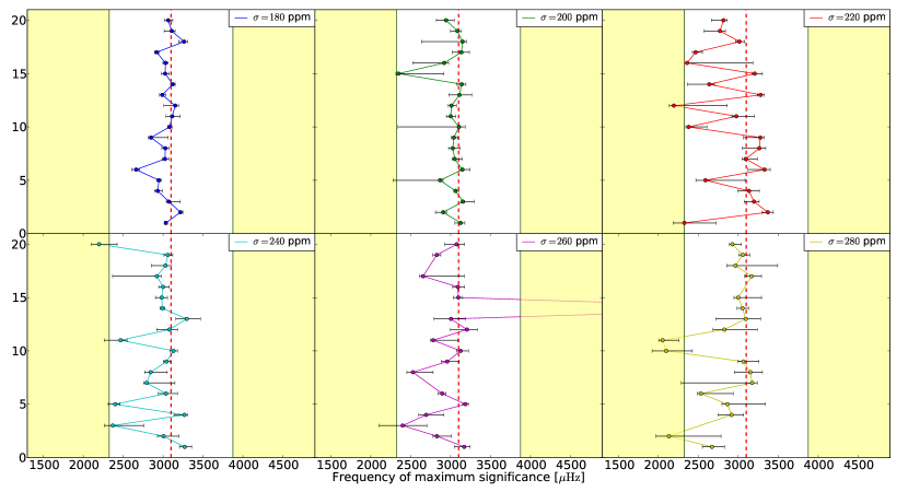
Figure 7: Estimated $\nu_{\rm max}$ values from the MWPS method, for different realizations of each noise level (see plot legends). Note that for the $\sigma=260$ and $280$ ppm only 18 points are plotted. This is due to the fact that both of these noise levels have two realisations which fall below detection at the 1 per cent level, as also indicated in Fig. 6

Panel (a) of Fig. 6 shows the $1/p_{\rm value}$ results from the MWPS tests. A detection is flagged as positive if the $1/p_{\rm value}$ is greater than 100 for $\alpha=0.01$ or 20 for $\alpha=0.05$, corresponding to the dashed red and blue lines respectively. For each of the noise levels the individual realisations are plotted with empty circles, and the median values for each of the noise realisations are marked by the red pentagons. The results for the PS$\otimes$PS method are shown in panels (b) and (c). Panel (b) shows the results from non-oversampled PS$\otimes$PS spectra, while panel (c) shows the results when oversampling by a factor 10 was used.

It is apparent that the MWPS returns a higher detection rate than the PS$\otimes$PS method, i.e., not only are the median detection rates higher, but there are also a much smaller fraction of non-detections. The MWPS also shows a much larger spread in the inferred $1/p_{\rm values}$, but as the values found in general give positive detections at a high significance level this is not a major cause for concern.

Since in our test data we know the location in frequency of the oscillations, we are also in a position to say something about the occurrence rate of false positive detections. Fig. 7 plots the position in frequency of flagged detections (at the one per cent level). The noise levels are indicated by the colour coded legend. The solar value of $\nu_{\rm max\odot}=3100\rm\ \mu Hz$ is marked by the dashed red line. The lines at 2325 and $3875\rm\ \mu Hz$ mark the interval we set for a correct positive detection. This interval corresponds to a one standard deviation of a Gaussian power envelope having $\nu_{\rm max}=3100\rm\ \mu Hz$. Points that fall in the shaded areas, outside this frequency range, might therefore be considered as putative false-positive detections. Only six realisations over the entire ensemble fell well within the shaded areas, three of which were from the highest noise case. Except for the false-positive in the $\sigma=260$ ppm case we find that in the remainder of the false-positive cases the MWPS is still picking up part of the underlying signal, but the central frequencies are offset due to beating with the noise. These cases could rightfully be seen as noise-affected detections rather than genuine false-positives. This suggests that even under quite extreme SNR conditions, the MWPS may still be used to ascertain if excess power is present, but the estimate for the actual $\nu_{\rm max}$ value should not be trusted in very high noise cases.

When at each noise level we calculate the difference between the estimated $\nu_{\rm max}$ and the true, underlying $\nu_{\rm max\odot}$, in units of the estimated uncertainties, we find that the fraction of detections that lie within $1\sigma$ of the true value stay fairly constant, at around 50 per cent. However, the average uncertainties do of course increase, reaching about 5 per cent at a noise level of $\sigma=260$. To put this fractional precision in the context of stellar properties estimation, consider, for example, the use of $\nu_{\rm max}$ to estimate $\log(g)$, via the scaling relation $\nu_{\rm max}\propto gT_{\rm eff}^{-0.5}$ (see, e.g., Brown et al. 1991; Kjeldsen & Bedding 1995). Under the assumption of superior precision in any complementary estimate of $T_{\rm eff}$, a fractional precision of 5 per cent in $\nu_{\rm max}$ equates to a similar fracitonal precision in $g$, and a precision of about 0.02 dex in $\log(g)$.

With a fraction of non-detections of only 10 per cent at $\sigma=280$ ppm we find (two realisations fall below detection at the 1 per cent level), as mentioned above, that the MWPS can be utilised at even higher noise levels to ascertain if excess power is present.

In most of the false-positive cases it is clear that there is an asymmetry in the estimated uncertainties on the central detection frequency, with the larger uncertainty pointing towards the true $\nu_{\rm max}$ value. In the bulk of these cases the asymmetry is caused by multiple peaks with nearly the same height in the mean $1/p_{\rm values}$ curve (supporting our contention that beating with the noise is to blame), where the highest peak happens to be at the low frequency end. The fact that the uncertainty goes mostly towards the true $\nu_{\rm max}$ value also supports our claim that part of the underlying signal is being picked up.

From looking at the results presented in Fig. 5, it is clear that, in the sense of determining an accurate estimate for $\nu_{\rm max}$, the PS$\otimes$PS method will be much better. This can be seen from the fact that the $1/p_{\rm values}$ peaks lie, in frequency, at the position of the $\Delta\nu/2$ value. The application of Eq. 14 would therefore return a value for $\nu_{\rm max}$ very close to the true value (under the assumption that the correct peak is used for the computation).

5 Conclusion

We have demonstrated that the MWPS method provides an efficient way of detecting excess power from solar-like oscillations under low signal-to-noise conditions, and that it also outperforms the frequently applied PS$\otimes$PS method. It is worth noting that while the efficiency of the PS$\otimes$PS will be affected by departures from near regularity of the mode spacings in frequency (e.g., in evolved solar-type stars showing mixed modes, or in stars showing significant variations of $\Delta\nu$ with frequency), such departures will not affect the performance of the MWPS method.

It is clear that the method is well suited as the initial step in the search for stellar oscillations in low SNR targets, and can provide useful information and guidelines as to where one should look more carefully for signatures of the near-regular frequency separations of the modes. It should also be evident that the greatest challenge for this otherwise relatively simple method is that of obtaining a reliable background fit, since inferences drawn rely on the implicit assumption that the fitted background is close to the actual, underlying background. We found that the introduction of the runs-test provided an extremely useful additional constraint to assess the robustness of the background fitting.

ACKNOWLEDGEMENTS

We would like to thank Andrea Miglio for checking the spread of the large separation $\Delta\nu$ about the used scaling relation.

WJC acknowledges the financial support of the UK Science and Technology Facilities Council (STFC). MNL thanks WJC and his colleagues for their hostpitality during two stays in Birmingham when the MWPS analysis was developed.

Funding for the Stellar Astrophysics Centre (SAC) is provided by The Danish National Research Foundation. The research is supported by the ASTERISK project (ASTERoseismic Investigations with SONG and Kepler) funded by the European Research Council (Grant agreement no.: 267864)

References

- [1] Appourchaux T., 2004, A&A, 428, 1039
- [2] Barlow R. J., Statistics: a guide to the use of statistical methods in the physical sciences, John Wiley and Sons, 1989
- [3] Borucki W. J. et al., 2010, Sci, 327, 977
- [4] Box, Hunter and Hunter, Statistics for experimenters: Design, Innovation, and Discovery , 2nd Edition, 2005, Wiley Series in Probability and Statistics
- [5] Brown T. M., Gilliland R. L., Noyes R. W., Ramsey L. W., 1991, ApJ, 368, 599
- [6] Campante T. L., Karoff C., Chaplin W. J., Elsworth Y. P., Handberg R., Hekker S., 2010, MNRAS, 408, 542
- [7] Chaplin W. J., Elsworth Y., Isaak G. R., Marchenkov K. I., Miller B. A., New R., Pinter B., Appourchaux T., 2002, MNRAS, 336, 979
- [8] Chaplin W. J. et al., 2011, ApJ, 732, 54
- [9] Frandsen S., Jones A., Kjeldsen H., Viskum M., Hjorth J., Andersen N. H., Thomsen B., 1995, A&A, 301, 123
- [10] Gilliland R. L. et al., PASP, 2010, 122, 131
- [11] Harvey J., 1985, in: Future Missions in Solar, Heliospheric and Space Plasma Physics, ESA Workshop, eds. E. Rolfe, B. Battrick, Noordwijk, Netherlands, p. 199
- [12] Hekker S. et al., 2010, MNRAS, 402, 2049
- [13] Huber D., Stello D., Bedding T. R., Chaplin W. J., Arentoft T., Quirion P.-O., Kjeldsen H., 2009, CoAst, 160, 74
- [14] Huber D. et al., 2011, ApJ, 743, 143
- [15] Karoff C., Campante T. L., Chaplin W. J., 2010, Astron. Nachr.
- [16] Kjeldsen H., 1992, Ph.D. Thesis, University of Aarhus, Denmark
- [17] Kjeldsen H., & Bedding T. R., 1995, A&A, 293, 87
- [18] Kjeldsen H., & Frandsen S., 1992, PASP, 104, 413
- [19] Koch D. G. et al., 2010, ApJ, 713, L79
- [20] Mathur S. et al., 2010, A&A, 511, 46
- [21] Mathur S. et al., 2011, ApJ, 741, 119
- [22] Mosser B., & Appourchaux T., 2009, A&A, 508, 877
- [23] Roca Cortès T. R., Jimènez A., Pallè P. L., and the GOLF and VIRGO teams, 1999, ESASP, 448, 135R
- [24] Savitzky A., & Golay, M. J. E., 1964, Analytical Chemistry, 36, 1627
- [25] Stello D. et al., 2007, MNRAS, 377, 584
- [26] Tassoul M., 1980, ApJS, 43, 469
- [27] Verner G. A., & Roxburgh I. W., 2011, Astron. Nachr.