Photon blockade induced by atoms with Rydberg coupling

Abstract

We study the photon blockade of two-photon scattering in a one-dimensional waveguide, which contains two atoms coupled via the Rydberg interaction. We obtain the analytic scattering solution of photonic wave packets with the Laplace transform method. We examine the photon correlation by addressing the two-photon relative wave function and the second-order correlation function in the single- and two-photon resonance cases. It is found that, under the single-photon resonance condition, photon bunching and antibunching can be observed in the two-photon transmission and reflection, respectively. In particular, the bunching and antibunching effects become stronger with the increasing of the Rydberg coupling strength. In addition, we find a phenomenon of bunching-antibunching transition caused by the two-photon resonance.

I Introduction

Controllable transport of photons in one-dimensional (1D) waveguides is crucial for realizing all-optical quantum devices, which are basic elements for implementation of photonic quantum information processing. As an example, a single-photon transistor Lukin2007 , controlling the propagation of a signal photon by another photon, can be used to implement a single-photon quantum switch. Up to now, there have been some proposals for coherent transport of single photons and two photons in waveguides with linear and nonlinear dispersion relations Fan2005 ; Fan2007 ; Zhou2008 ; Law2008 ; Liao2009 ; Gong2008 ; Chang2011 ; Shi2009 ; Shi_LSZ ; Tsoi2009 ; Liao2010A ; Liao2010B ; Shi2012 ; Rephaeli2011 ; Xu2010 ; Roy2010 ; Baranger2012 . Most of them are based on the physical mechanism of photon scattering by tunable targets.

Two-photon transport in a waveguide is a nontrivial mission since nonlinear photon-photon interaction Imamoglu1997 ; Kimble2005 may be induced by nonlinear scattering targets such as a Kerr-type nonlinear cavity Liao2010B or strongly interacting atoms Vuletic2012 . In particular, there exists a kind of induced photon nonlinearity that can lead to photon blockade Imamoglu1997 ; Kimble2005 , which can be used to realize single-photon sources. This photon nonlinearity in a cavity containing atoms is a second-order effect of the interactions between the cavity field and the atoms therein Imamoglu1997 , thus it is quite natural to ask how could the atoms directly mediate such a nonlinearity for photon blockade. Recently, Shi et al. Shi2011 have considered two-photon scattering in a waveguide coupled to a cavity containing a two-level atom. Their results on photon blockade can well fit the experiment data Kimble2005 .

We note that the blockade effect can also occur among atoms. In atomic blockade, double excitation of atoms is strongly suppressed by some direct Lukin2000 ; Lukin2001 ; Tong2004 ; Saffman2009 ; Grangier2009 and indirect Huang2012 interatom coupling. Physically, when the interaction between excited atoms is strong enough, it will be difficult to simultaneously excite two atoms due to the excess coupling-energy requirement. Since the simultaneous excitation of two atoms needs to absorb two photons, the atomic blockade will suppress the simultaneous two-photon absorption. Then the absorbed photons can only be emitted one by one. In other words, the atomic blockade can induce the photon blockade under certain conditions. With this motivation, we will investigate in this paper how the atomic blockade Lukin2001 ; Lukin2001 ; Tong2004 ; Saffman2009 ; Grangier2009 ; Adams2010 ; Buchler2011 ; Lukin2011 ; Molmer2012 ; Huang2012 exerts an influence on the photon blockade Imamoglu1997 ; Kimble2005 .

Deeply understanding the relation between these two kinds of blockade effect (atomic blockade and photon blockade) will provide a straightforward way to probe the nature of the inter-atom coupling through photon blockade effect. It is also possible to display the atomic blockade effect due to the photon blockade phenomenon. To illustrate the physical mechanism behind these scientific and technical issues, we study the spatial-wave-packet transport of two photons in a 1D linear waveguide, which contains two intercoupled two-level Rydberg atoms. To understand the single-photon contributions in the two-photon process, we first calculate spatial evolution of the single-photon wave packet. The similar approach has been used in Refs. Liao2010B ; Tsoi2009 to study the scattering problem for spatial wave packets. Then, we calculate the evolution of the spatial wave packet for two photons. Since the second-order correlation function $g^{(2)}$ can describe the photon-blockade effect, we calculate $g^{(2)}$ for both the reflected and transmitted photons. We find that the $g^{(2)}$ is proportional to the relative spatial distribution probability of the two photons with some distance. We can predict the photon statistical properties from the wave function of the two photons. Our calculation shows that the spatial distribution of the two photons is strongly dependent on the interatom coupling strength, where we have employed the direct Rydberg coupling between the two atoms. The transmitted photons are strongly bunched except for some special Rydberg coupling strength, which depends on the initial conditions. The reflected photons are strongly repulsed by each other, namely the photon-blockade effect, when Rydberg coupling strength is away from the two-photon resonance, which means the Rydberg coupling strength equals the sum of each photon’s center detuning. Here, the center detuning denotes the deviation of the frequency center for single input wave packet from the atomic transition frequency. On the contrary, at this two-photon resonance, the two reflected photons exhibits bunching behavior. We can use this sole bunching behavior for the reflected two photons to probe the nature of the interatom coupling.

This paper is organized as follows. In Sec. II, we introduce the physical model and its Hamiltonian. In Secs. III and IV, we solve the single- and two-photon scattering problem with the Laplace transform, respectively. In particular, we describe the two-photon correlation in the two-photon relative coordinate space, and calculate the second-order correlation function for the two reflected or transmitted photons. Finally, we draw our conclusion in Sec. V and present the detailed derivations for the two-photon solution in the Appendix.

II Model setup

We start by considering a $1$D linear waveguide, which contains two two-level atoms coupled via the Rydberg interaction (see Fig. 1). The model Hamiltonian (with $\hbar=1$) of the system reads as

$$\hat{H} = \int_{0}^{\infty}dk\omega_{k}(\hat{r}_{k}^{\dagger}\hat{r}_{k}+\hat{l}_{k}^{\dagger}\hat{l}_{k})+\frac{\omega_{0}}{2}(\hat{\sigma}_{1}^{z}+\hat{\sigma}_{2}^{z})$$ (1)

$$+g_{0}\int_{0}^{\infty}dk\sum_{\ell=1,2}[\hat{\sigma}_{\ell}^{+}(\hat{r}_{k}+\hat{l}_{k})+(\hat{r}_{k}^{\dagger}+\hat{l}_{k}^{\dagger})\hat{\sigma}_{\ell}^{-}]$$

$$+\xi|e\rangle_{1}\langle e|_{1}\otimes|e\rangle_{2}\langle e|_{2}.$$

The first line of Eq. (1) is the free Hamiltonian of the fields and atoms. The creation (annihilation) operators $\hat{r}_{k}^{\dagger}$ ($\hat{r}_{k}$) and $\hat{l}_{k}^{\dagger}$ ($\hat{l}_{k}$) describe, respectively, the right- and left-propagating light fields in the waveguide, with wave vector $k$ and frequency $\omega_{k}=\upsilon_{p}k$ (hereafter we take the group velocity of light $\upsilon_{p}=1$). Pauli’s operators $\hat{\sigma}_{\ell}^{x,y,z}$ [$\hat{\sigma}_{\ell}^{\pm}=\frac{1}{2}(\hat{\sigma}_{\ell}^{x}\pm i\hat{\sigma}_{\ell}^{y})$] are introduced to represent the $\ell$th ($\ell=1,2$) atom with energy level spacing $\omega_{0}$. The Hamiltonian in the second line of Eq. (1) depicts the atom-field interaction with the coupling strength $g_{0}$. In addition, the last term in Eq. (1) stands for the Rydberg interaction of strength $\xi$ between the Rydberg states $|e\rangle_{\ell}$ ($\ell=1,2$) of each atom Lukin2001 ; Adams2010 ; Cote2002 ; Marinescu1997 ; Weidemuller2010 ; Grangier2012 ; Wu2011 . Physically, this Rydberg coupling strength $\xi$ depends on the distance $r$ between the two atoms. For the dipole-dipole and van der Waals interactions, the strength $\xi$ takes the form $\xi\sim 1/r^{3}$ and $\xi\sim 1/r^{6}$, respectively. When the distance is on the order of a few $\mu$m, $\xi$ could be very strong Grangier2012 . Since the coordinates of the two atoms are external parameters rather than dynamical variables, we use the strength $\xi$ to characterize the Rydberg interaction.

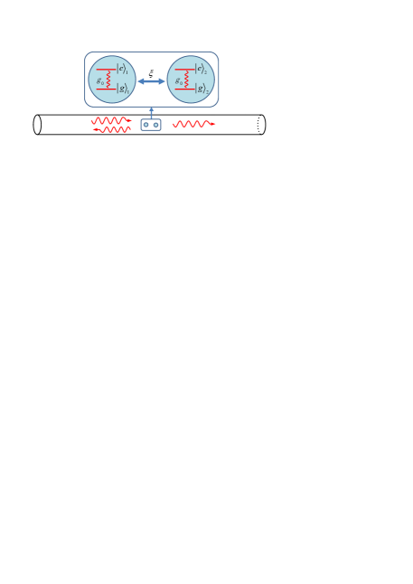
Figure 1: Schematic diagram of the physical setup. Two interacting atoms are placed in a 1D linear waveguide. Photons injected from the left-hand side of the waveguide are scattered by the atoms.

By introducing the even- and odd-parity modes,

$$\hat{b}_{k}=\frac{1}{\sqrt{2}}(\hat{r}_{k}+\hat{l}_{k}),\hskip 28.45274pt\hat{c}_{k}=\frac{1}{\sqrt{2}}(\hat{r}_{k}-\hat{l}_{k}),$$ (2)

the Hamiltonian $\hat{H}=\hat{H}^{(o)}+\hat{H}^{(e)}$ can be decomposed into two parts, the odd-parity part $\hat{H}^{(o)}=\int_{0}^{\infty}dk\omega_{k}\hat{c}_{k}^{\dagger}\hat{c}_{k}$ and the even-parity part,

$$\hat{H}^{(e)} = \int_{0}^{\infty}dk\omega_{k}\hat{b}_{k}^{\dagger}\hat{b}_{k}+\frac{\omega_{0}}{2}(\hat{\sigma}_{1}^{z}+\hat{\sigma}_{2}^{z})$$ (3)

$$+g\int_{0}^{\infty}dk[(\hat{\sigma}_{1}^{+}+\hat{\sigma}_{2}^{+})\hat{b}_{k}+\hat{b}_{k}^{\dagger}(\hat{\sigma}_{1}^{-}+\hat{\sigma}_{2}^{-})]$$

$$+\xi|e\rangle_{1}\langle e|_{1}\otimes|e\rangle_{2}\langle e|_{2},$$

where $g=\sqrt{2}g_{0}$. Obviously, the odd-parity modes decouple with the atoms so that their evolution is free. In the following we will mainly deal with the evolution of the even-parity modes.

In a rotating frame with respect to

$$\hat{H}_{0}^{(e)}=\omega_{0}\int_{0}^{\infty}dk\hat{b}_{k}^{\dagger}\hat{b}_{k}+\frac{\omega_{0}}{2}(\hat{\sigma}_{1}^{z}+\hat{\sigma}_{2}^{z}),$$ (4)

the Hamiltonian $\hat{H}^{(e)}$ becomes

$$\hat{H}_{I}^{(e)} = \int_{0}^{\infty}dk\Delta_{k}\hat{b}_{k}^{\dagger}\hat{b}_{k}+\xi|e\rangle_{1}\langle e|_{1}\otimes|e\rangle_{2}\langle e|_{2}$$ (5)

$$+g\int_{0}^{\infty}dk[(\hat{\sigma}_{1}^{+}+\hat{\sigma}_{2}^{+})\hat{b}_{k}+\hat{b}_{k}^{\dagger}(\hat{\sigma}_{1}^{-}+\hat{\sigma}_{2}^{-})],$$

where $\Delta_{k}=\omega_{k}-\omega_{0}$. Based on Hamiltonian (5), we can work out the photon scattering solution for the system. To understand the physical picture for the photon scattering, we will first consider the single-photon scattering, and then we will study how the Rydberg interaction affects the two-photon scattering.

III Single-photon scattering

In the following discussions, we will employ the dynamical approach Tsoi2009 ; Liao2010B rather than the stationary-state approach Gong2008 ; Shi2009 ; Zhou2008 ; Chang2011 ; Xu2010 ; Fan2007 ; Fan2005 to study the photon-scattering problem. We note that the total-excitation-number operator $\hat{N}=\hat{a}^{\dagger}\hat{a}+|e\rangle_{1}\langle e|_{1}+|e\rangle_{2}\langle e|_{2}$ in this system is a conserved quantity due to $[\hat{N},\hat{H}_{I}^{(e)}]=0$. Consequently, the Hilbert space of the system can be divided into the direct-sum subspaces with different excitations. For single-photon scattering, it is sufficient to consider the scattering problems within the single-excitation subspace. In this subspace, an arbitrary state of the system can be expressed as

$$|\Phi(t)\rangle = \alpha_{1}(t)|\emptyset\rangle|e\rangle_{1}|g\rangle_{2}+\alpha_{2}(t)|\emptyset\rangle|g\rangle_{1}|e\rangle_{2}$$ (6)

$$+\int_{0}^{\infty}dk\beta_{k}(t)\hat{b}_{k}^{\dagger}|\emptyset\rangle|g\rangle_{1}|g\rangle_{2},$$

where $|\emptyset\rangle$ is the vacuum state and $|1_{k}\rangle$ represents the state with a single photon in the $k$th even mode of the waveguide. The variables $\alpha_{1}(t)$, $\alpha_{2}(t)$, and $\beta_{k}(t)$ are probability amplitudes. By solving the Schrödinger equation $i\left(\partial/\partial t\right)|\Phi(t)\rangle=\hat{H}_{I}^{(e)}|\Phi(t)\rangle$, we obtain the following equations of motion for probability amplitudes:

$$\dot{\alpha}_{1}(t) = -ig\int_{0}^{\infty}dk\beta_{k}(t),$$

$$\dot{\alpha}_{2}(t) = -ig\int_{0}^{\infty}dk\beta_{k}(t),$$

$$\dot{\beta}_{k}(t) = -i\Delta_{k}\beta_{k}(t)-ig[\alpha_{1}(t)+\alpha_{2}(t)].$$ (7)

For single-photon scattering, we assume that the two atoms are initially in ground state and a single even-mode photon is in a Lorentzian wave packet. The initial condition reads

$$\alpha_{1}(0) = 0,\hskip 22.76228pt\alpha_{2}(0)=0,$$

$$\beta_{k}(0) = G_{1}\frac{e^{i\Delta_{k}l}}{\Delta_{k}-\delta+i\epsilon},\hskip 22.76228ptl\geq 0,$$ (8)

where $G_{1}=\sqrt{\epsilon/\pi}$ is the normalization constant, and $l$ is the initial distance between the wavefront of the photon wave packet and the atoms. In addition, $\delta$ and $\epsilon$ are, respectively, the center detuning and width of the wave packet. The transient solution of these probability amplitudes might be obtained using the Laplace transform method. For the scattering problem, we focus on the long-time solution,

$$\alpha_{1}(t\rightarrow\infty) = 0,\hskip 22.76228pt\alpha_{2}(t\rightarrow\infty)=0,$$

$$\beta_{k}(t\rightarrow\infty) = \bar{t}_{k}\beta_{k}(0)e^{-i\Delta_{k}t},$$ (9)

where we introduce the phase factor

$$\bar{t}_{k}=\frac{\Delta_{k}-i\gamma}{\Delta_{k}+i\gamma}$$ (10)

with $\gamma=2\pi g^{2}$ being the decay rate of each atom. It follows from Eq. (9) that the single photon with wave vector $k$ only picks up a phase shift $\varphi_{k}$ defined by $\exp{(i\varphi_{k})}=\bar{t}_{k}$ after being scattered by the two atoms.

In practice, a single photon should be injected in right- or left-propagating modes. Hence, we need to consider the single-photon scattering in modes $\hat{r}_{k}$ and $\hat{l}_{k}$. For the right-propagating single-photon injection, the initial state is

$$|\psi(0)\rangle = \int_{0}^{\infty}dk\beta_{k}(0)\hat{r}_{k}^{\dagger}|\emptyset\rangle$$ (11)

$$= \frac{1}{\sqrt{2}}\int_{0}^{\infty}dk\beta_{k}(0)(\hat{b}_{k}^{\dagger}+\hat{c}_{k}^{\dagger})|\emptyset\rangle.$$

The injected single-photon wave function in position space reads

$$\langle x|\psi(0)\rangle\simeq-i\sqrt{2\pi}G_{1}e^{i(\delta-i\epsilon)(x+l)}\theta(-x-l),$$ (12)

where $\theta(x)$ is the Heaviside step function. In the long-time limit, the single-photon wave function in $k$ space is

$$|\psi(t\rightarrow\infty)\rangle = \int_{0}^{\infty}dk\beta_{k}(0)e^{-i\Delta_{k}t}(T_{k}\hat{r}_{k}^{\dagger}+R_{k}\hat{l}_{k}^{\dagger})|\emptyset\rangle,$$

where the transmission and reflection amplitudes are obtained as

$$T_{k}=\frac{\Delta_{k}}{\Delta_{k}+i\gamma},\hskip 22.76228ptR_{k}=\frac{-i\gamma}{\Delta_{k}+i\gamma}.$$ (14)

The above result has been reported in Refs. Fan2005 ; Liao2010B . At the resonant case, i.e., $\Delta_{k}=0$, we get $T_{k}=0$ and $R_{k}=-1$, which means that the single photon is completely reflected. This complete reflection can be explained based on quantum interference. In the resonant case, the coherent amplitude for transmitted (reflected) photons disappears (increases) due to destructive (constructive) interference between the photon injection and the atom emission channels.

The output wave function in position space is

$$\langle x|\psi(t\rightarrow\infty)\rangle = \psi_{r}(x,l,\delta)+\psi_{l}(x,l,\delta),$$ (15)

where

$$\psi_{r}(x,l,\delta) = -i\sqrt{2\pi}G_{1}T_{\delta-i\epsilon}e^{i(\delta-i\epsilon)(x-t+l)}\theta(-x+t-l),$$

$$\psi_{l}(x,l,\delta) = -i\sqrt{2\pi}G_{1}R_{\delta-i\epsilon}e^{-i(\delta-i\epsilon)(x+t-l)}\theta(x+t-l).$$

We note that the output waveforms (proportional to $|\psi_{r}(x,l,\delta)|^{2}$ and $|\psi_{l}(x,l,\delta)|^{2}$) of the transmitted and reflected photons are the same as that of the input state (12), except for their normalized amplitudes by the transmission and reflection coefficients ($|T_{\delta-i\epsilon}|^{2}$ and $|R_{\delta-i\epsilon}|^{2}$), respectively.

IV Two-photon scattering

We now turn to the two-photon scattering. We will use the Laplace transform to obtain the long-time state of two photons, and special attention will be paid to clarifying the relationship between the atom blockade and the photon blockade.

IV.1 Equations of motion and solution

In the two-excitation subspace, there are four types of basis state: two excitations in atoms (with basis $|\emptyset\rangle|e\rangle_{1}|e\rangle_{2}$), one excitation in atoms and the other in light fields (with bases $|1_{k}\rangle|e\rangle_{1}|g\rangle_{2}$ and $|1_{k}\rangle|g\rangle_{1}|e\rangle_{2}$), and two excitations in light fields (with basis $|1_{p},1_{q}\rangle|g\rangle_{1}|g\rangle_{2}$). Then an arbitrary state in this subspace is written as

$$|\varphi(t)\rangle = A(t)|\emptyset\rangle|e\rangle_{1}|e\rangle_{2}+\int_{0}^{\infty}dkB_{k}(t)\hat{b}^{\dagger}_{k}|\emptyset\rangle|e\rangle_{1}|g\rangle_{2}$$ (17)

$$+\int_{0}^{\infty}dkC_{k}(t)\hat{b}^{\dagger}_{k}|\emptyset\rangle|g\rangle_{1}|e\rangle_{2}$$

$$+\int_{0}^{\infty}dp\int_{0}^{p}dqD_{p,q}(t)\hat{b}^{\dagger}_{p}\hat{b}^{\dagger}_{q}|\emptyset\rangle|g\rangle_{1}|g\rangle_{2},$$

where $A(t)$, $B_{k}(t)$, $C_{k}(t)$, and $D_{p,q}(t)$ are probability amplitudes. By solving the Schrödinger equation, we get the following equations of motion for these probability amplitudes:

$$\dot{A}(t) = -i\xi A(t)-ig\int_{0}^{\infty}dk[B_{k}(t)+C_{k}(t)],$$

$$\dot{B}_{k}(t) = -i\Delta_{k}B_{k}(t)-igA(t)-ig\int_{0}^{\infty}dpD_{p,k}(t),$$

$$\dot{C}_{k}(t) = -i\Delta_{k}C_{k}(t)-igA(t)-ig\int_{0}^{\infty}dpD_{p,k}(t),$$

$$\dot{D}_{p,q}(t) = -i(\Delta_{p}+\Delta_{q})D_{p,q}(t)-ig[B_{p}(t)+B_{q}(t)]$$ (18)

$$-ig[C_{p}(t)+C_{q}(t)],$$

where we have used the symmetry relation $D_{k,p}(t)=D_{p,k}(t)$.

We consider the initial state where the two atoms are in their ground state and the two photons are in a wave packet. The corresponding initial condition reads

$$A(0) = 0,\hskip 22.76228ptB_{k}(0)=0,\hskip 22.76228ptC_{k}(0)=0,$$

$$D_{p,q}(0) = G_{2}\left(\frac{e^{i\Delta_{p}l_{1}}}{\Delta_{p}-\delta_{1}+i\epsilon}\frac{e^{i\Delta_{q}l_{2}}}{\Delta_{q}-\delta_{2}+i\epsilon}\right.$$ (19)

$$\left.+\frac{e^{i\Delta_{q}l_{1}}}{\Delta_{q}-\delta_{1}+i\epsilon}\frac{e^{i\Delta_{p}l_{2}}}{\Delta_{p}-\delta_{2}+i\epsilon}\right),$$

where $l_{\ell}$ is the initial position of the $\ell$th ($\ell=1,2$) photon. Without loss of generality, we assume $l_{1}\geq 0$, $l_{2}\geq 0$, and $l_{1}\geq l_{2}$. The normalization constant reads

$$G_{2}=\frac{\epsilon}{\pi}\left[1+\frac{4\epsilon^{2}e^{-2\epsilon\left(l_{1}-l_{2}\right)}}{\left(\delta_{1}-\delta_{2}\right)^{2}+4\epsilon^{2}}\right]^{-1/2}.$$ (20)

Under the above initial condition, the long-time solution for these probability amplitudes can be obtained as $A(t\rightarrow\infty)=0$, $B_{k}(t\rightarrow\infty)=0$, $C_{k}(t\rightarrow\infty)=0$, and

$$D_{p,q}(t\rightarrow\infty) = [\bar{t}_{p}\bar{t}_{q}D_{p,q}(0)+J_{p,q}]e^{-i(\Delta_{p}+\Delta_{q})t},$$ (21)

where $\bar{t}_{p}$ $(\bar{t}_{q})$ has been defined by Eq. (10) and

$$J_{p,q} = 4G_{2}\gamma^{2}\frac{e^{i(\Delta_{p}+\Delta_{q})l_{1}}}{(\Delta_{p}+i\gamma)(\Delta_{q}+i\gamma)}\frac{(\Delta_{p}+\Delta_{q}-2\xi)}{(\Delta_{p}+\Delta_{q}-\xi+i\gamma)}$$ (22)

$$\times\frac{1}{(\Delta_{p}+\Delta_{q}-\delta_{1}-\delta_{2}+2i\epsilon)}$$

$$\times\left[\left(\frac{e^{-(i\delta_{2}+\epsilon)(l_{1}-l_{2})}}{i\gamma+\delta_{2}-i\epsilon}+\frac{e^{-(i\delta_{2}+\epsilon)(l_{1}-l_{2})}}{\Delta_{p}+\Delta_{q}-\delta_{2}+i\epsilon+i\gamma}\right)\right.$$

$$\left.-\left(\frac{e^{-\gamma(l_{1}-l_{2})}}{i\gamma+\delta_{2}-i\epsilon}-\frac{e^{-\gamma(l_{1}-l_{2})}}{\Delta_{p}+\Delta_{q}-\delta_{1}+i\epsilon+i\gamma}\right)\right].$$

The first term in Eq. (21) describes two-photon independent scattering process, while the second term represents photon correlation induced by scattering process. It should be pointed out that, when $\xi=0$, $J_{p,q}\neq 0$. This fact means that the photon correlation can be observed even in the absence of the Rydberg interaction. Physically, this residual photon correlation is generated due to the quantum interference between the two transition channels of the two atoms. A similar result has been shown in Ref. Rephaeli2011 .

IV.2 Two-photon wave functions in real space

We consider a realistic case with the two photons injected from the left-hand side of the waveguide. Then, the initial state of the photons can be written as

$$|\psi(0)\rangle = \int_{0}^{\infty}dp\int_{0}^{p}dqD_{p,q}(0)\hat{r}_{p}^{\dagger}\hat{r}_{q}^{\dagger}|\emptyset\rangle.$$ (23)

In terms of the basis wave function

$$\langle x_{1},x_{2}|\hat{r}_{p}^{\dagger}\hat{r}_{q}^{\dagger}|0\rangle=\mathcal{N}_{rr}\left(e^{i\Delta_{p}x_{1}}e^{i\Delta_{q}x_{2}}+x_{1}\leftrightarrow x_{2}\right)$$ (24)

with $\mathcal{N}_{rr}=1/(2\sqrt{2}\pi)$, the wave function in position space of the initial state is

$$\langle x_{1},x_{2}|\psi(0)\rangle = -4\pi^{2}\mathcal{N}_{rr}G_{2}e^{(i\delta_{1}+\epsilon)(x_{1}+l_{1})}e^{(i\delta_{2}+\epsilon)(x_{2}+l_{2})}$$ (25)

$$\times\theta(-x_{1}-l_{1})\theta(-x_{2}-l_{2})+(x_{1}\leftrightarrow x_{2}).$$

By introducing the center-of-mass coordinate $x_{c}=(x_{1}+x_{2})/2$, relative coordinate $x=x_{1}-x_{2}$, total center-detuning $E=\delta_{1}+\delta_{2}$, and relative center detuning $\delta=(\delta_{1}-\delta_{2})/2$, the wave function (25) becomes

$$\langle x_{1},x_{2}|\psi(0)\rangle = -4\pi^{2}\mathcal{N}_{rr}G_{2}\left[e^{i\delta_{1}(x_{c}+x/2+l_{1})}e^{\epsilon(x_{c}+x/2+l_{1})}\right.$$ (26)

$$\left.\times e^{i\delta_{2}(x_{c}-x/2+l_{2})}e^{\epsilon(x_{c}-x/2+l_{2})}\right.$$

$$\times\left.\theta(-x_{c}+x/2-l_{2})\theta(-x_{c}-x/2-l_{1})\right.$$

$$\left.+(x\leftrightarrow-x)\right].$$

For the special case of $l_{2}=l_{1}$, the wave function reduces to

$$\langle x_{1},x_{2}|\psi(0)\rangle = -8\pi^{2}\mathcal{N}_{rr}G_{2}e^{(iE+2\epsilon)(x_{c}+l_{1})}$$ (27)

$$\times\cos(\delta x)\theta(-x_{c}-l_{1}-|x|/2).$$

After being scattered by the two Rydberg atoms, the state of the two photons in the long-time limit can be expressed as

$$|\psi(t\rightarrow\infty)\rangle = |\psi_{rr}\rangle+|\psi_{rl}\rangle+|\psi_{lr}\rangle+|\psi_{ll}\rangle,$$ (28)

where

$$|\psi_{rr}\rangle = \int_{0}^{\infty}\int_{0}^{\infty}dpdqD_{p,q}^{rr}e^{-i(\Delta_{p}+\Delta_{q})t}\hat{r}_{p}^{\dagger}\hat{r}_{q}^{\dagger}|\emptyset\rangle,$$

$$|\psi_{rl}\rangle = \int_{0}^{\infty}\int_{0}^{\infty}dpdqD_{p,q}^{rl}e^{-i(\Delta_{p}+\Delta_{q})t}\hat{r}_{p}^{\dagger}\hat{l}_{q}^{\dagger}|\emptyset\rangle,$$

$$|\psi_{lr}\rangle = \int_{0}^{\infty}\int_{0}^{\infty}dpdqD_{p,q}^{lr}e^{-i(\Delta_{p}+\Delta_{q})t}\hat{l}_{p}^{\dagger}\hat{r}_{q}^{\dagger}|\emptyset\rangle,$$

$$|\psi_{ll}\rangle = \int_{0}^{\infty}\int_{0}^{\infty}dpdqD_{p,q}^{ll}e^{-i(\Delta_{p}+\Delta_{q})t}\hat{l}_{p}^{\dagger}\hat{l}_{q}^{\dagger}|\emptyset\rangle,$$ (29)

with

$$D_{p,q}^{rr} = \frac{1}{2}(T_{p}T_{q}D_{p,q}(0)+J_{p,q}/4),$$

$$D_{p,q}^{rl} = \frac{1}{2}(T_{p}R_{q}D_{p,q}(0)+J_{p,q}/4),$$

$$D_{p,q}^{lr} = \frac{1}{2}(R_{p}T_{q}D_{p,q}(0)+J_{p,q}/4),$$

$$D_{p,q}^{ll} = \frac{1}{2}(R_{p}R_{q}D_{p,q}(0)+J_{p,q}/4).$$ (30)

Here, $D_{p,q}^{rr}$ and $D_{p,q}^{ll}$ are, respectively, the two-photon transmission and reflection amplitudes. In addition, $D_{p,q}^{rl}$ ($D_{p,q}^{lr}$) relates to the process where the photon with wave number $p$ ($q$) is transmitted into the right-propagation mode and the photon with wave number $q$ ($p$) is reflected into the left-propagation mode.

IV.3 Two-photon correlation in position variables

To characterize the photon correlation, we will consider the two-photon transmission and reflection cases. For the two-photon transmission, the output state of the two right-going photons is

$$\langle x_{1},x_{2}|\psi_{rr}\rangle = -4\pi^{2}\mathcal{N}_{rr}G_{2}e^{i(E-2i\epsilon)(x_{c}-t)}$$ (31)

$$\times e^{i(E/2-i\epsilon)(l_{1}+l_{2})}e^{i\delta(l_{1}-l_{2})}\Phi_{rr}(x)$$

with

$$\Phi_{rr}(x) = T_{\delta_{1}-i\epsilon}T_{\delta_{2}-i\epsilon}[e^{i\delta x}\theta(-x_{c}-x/2+t-l_{1})$$ (32)

$$\times\theta(-x_{c}+x/2+t-l_{2})+x\leftrightarrow-x]$$

$$-R_{\delta_{1}-i\epsilon}R_{\delta_{2}-i\epsilon}\frac{E-2i\epsilon-2\xi}{E-2i\epsilon-\xi+i\gamma}$$

$$\times e^{i(E/2-i\epsilon+i\gamma)|x|}\theta(-x_{c}+t-|x|/2-l_{1}).$$

When $l_{2}=l_{1}$, the output state (31) reduces to

$$\langle x_{1},x_{2}|\psi_{rr}\rangle = -8\pi^{2}\mathcal{N}_{rr}G_{2}e^{(iE+2\epsilon)(x_{c}-t+l_{1})}$$ (33)

$$\times\theta(-x_{c}+t-l_{1}-|x|/2)\phi_{rr}(x),$$

where

$$\phi_{rr}(x) = T_{\delta_{1}-i\epsilon}T_{\delta_{2}-i\epsilon}\cos(\delta x)$$

$$-\frac{1}{2}R_{\delta_{1}-i\epsilon}R_{\delta_{2}-i\epsilon}\frac{E-2\xi-2i\epsilon}{E-\xi-2i\epsilon+i\gamma}e^{i(E/2-i\epsilon+i\gamma)|x|},$$

which satisfies $\phi_{rr}(-x)=\phi_{rr}(x)$. In the derivation of Eq. (31), we have used the condition $\gamma\gg\epsilon$.

We note that Eq. (33) is a product of the center-of-mass wave function $\exp[(iE+2\epsilon)(x_{c}-t+l_{1})]$ and the relative wave function $\phi_{rr}(x)$ in the region defined by the step function $\theta(-x_{c}+t-l_{1}-|x|/2)$. As $|\phi_{rr}(x)|^{2}$ is proportional to the joint probability for two photons with a separation $x$, it could be used to characterize the spatial statistics of the two photons. For example, the peak and dip feature of $|\phi_{rr}(x)|^{2}$ around zero distance $x=0$, implies photon bunching and antibunching, respectively. In Eq. (LABEL:eq:psiR2), the first term of $\phi_{rr}(x)$ describes an independent two-photon transmission process, while the second term is a two-photon correlation induced by scattering. Physically, the present system has two resonant scattering conditions: single- and two-photon resonances. When the frequency center of a single-photon wave packet matches the energy separation of a single atom, i.e. $\delta_{1}=\delta_{2}=0$ (or $E=0$ and $\delta=0$), the single photon will resonantly excite the atom. We call this as the single-photon resonance condition. On the other hand, when the total center detuning of the two photons equals to the energy shift due to the Rydberg coupling, i.e., $\delta_{1}+\delta_{2}=\xi$ (or $E=\xi$), the two photons can resonantly excite the two coupled atoms, even the single-photon process could be off-resonant. This regime is called two-photon resonance.

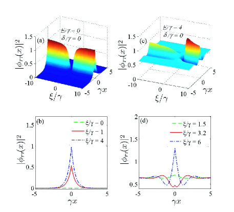
Figure 2: (Color online) Plots of $|\phi_{rr}(x)|^{2}$ vs the scaled parameters $\xi/\gamma$ and $\gamma x$ when (a) $E/\gamma=0$, $\delta=0$ and (b) $E/\gamma=4$, $\delta=0$. (c) and (d) show, respectively, the curves from (a) and (b) when the parameter $\xi/\gamma$ takes several certain values. Here, we consider the near monochromatic limit $\epsilon/\gamma=0.01$.

In the single-photon resonance case, the independent two-photon transmission process will be completely suppressed, and a pure photon-correlation effect can be seen from $|\phi_{rr}(x)|^{2}$. In Fig. 2(a), we plot $|\phi_{rr}(x)|^{2}$ as a function of $\xi/\gamma$ and $\gamma x$. When $\xi=0$, there is no photon correlation [dashed line in Fig. 2(b)]. This result corresponds to the fluorescence-complete-vanishing phenomenon found in Ref. Rephaeli2011 . For a nonzero $\xi/\gamma$, we can see clear evidence for photon bunching [Fig. 2(b)]. In particular, with the increasing of $\xi/\gamma$, $|\phi_{rr}(0)|^{2}$ increases gradually, and saturates when $\xi/\gamma\gg 1$. This means that the photon bunching becomes stronger for a larger $\xi/\gamma$ in the single-photon resonance regime.

In the case of single-photon off resonance (e.g., $E/\gamma=4$), we plot $|\phi_{rr}(x)|^{2}$ vs $\xi/\gamma$ and $\gamma x$ in Figs. 2(c) and 2(d). The curves exhibit photon bunching in most regions of $\xi/\gamma$, but there is also some oscillation pattern with respect to $\gamma x$ due to independent photon transmission. However, around the two-photon resonance, i.e., $\xi=E$, there is a clear evidence for the photon antibunching [Fig. 2(d)]. This interesting phenomenon of photon statistics transition from bunching to antibunching is induced by the two-photon resonance.

Similarly, using the basis wave function

$$\langle x_{1},x_{2}|\hat{l}_{p}^{\dagger}\hat{l}_{q}^{\dagger}|0\rangle=\mathcal{N}_{ll}\left(e^{-i\Delta_{p}x_{1}}e^{-i\Delta_{q}x_{2}}+x_{1}\leftrightarrow x_{2}\right)$$ (35)

with $\mathcal{N}_{ll}=1/(2\sqrt{2}\pi)$, the output state of the two left-going photons in the long-time limit $t\rightarrow\infty$ is

$$\langle x_{1},x_{2}|\psi_{ll}\rangle = -4\pi^{2}\mathcal{N}_{ll}G_{2}e^{i(E/2-i\epsilon)(l_{1}+l_{2})}e^{i\delta(l_{1}-l_{2})}$$ (36)

$$\times e^{i(E-2i\epsilon)(-x_{c}-t)}\Phi_{ll}(x)$$

with

$$\Phi_{ll}(x) \equiv R_{\delta_{1}-i\epsilon}R_{\delta_{2}-i\epsilon}[e^{-i\delta x}\theta(x_{c}+x/2+t-l_{1})$$ (37)

$$\times\theta(x_{c}-x/2+t-l_{2})+x\leftrightarrow-x]$$

$$-R_{\delta_{1}-i\epsilon}R_{\delta_{2}-i\epsilon}\frac{E-2i\epsilon-2\xi}{E-2i\epsilon-\xi+i\gamma}$$

$$\times e^{i(E/2-i\epsilon+i\gamma)|x|}\theta(x_{c}+t-|x|/2-l_{1}).$$

When $l_{1}=l_{2}$, the output state of two reflected photons becomes

$$\langle x_{1},x_{2}|\psi_{ll}\rangle = -8\pi^{2}\mathcal{N}_{ll}G_{2}e^{(iE+2\epsilon)(-x_{c}-t+l_{1})}$$ (38)

$$\times\theta(x_{c}+t-l_{1}-|x|/2)\phi_{ll}(x)$$

with

$$\phi_{ll}(x) = R_{\delta_{1}-i\epsilon}R_{\delta_{2}-i\epsilon}\left[\cos(\delta x)\right.$$ (39)

$$\left.-\frac{1}{2}\frac{E-2i\epsilon-2\xi}{E-2i\epsilon-\xi+i\gamma}e^{i(\frac{E}{2}-i\epsilon+i\gamma)|x|}\right].$$

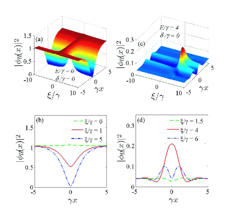
Figure 3: (Color online) Plots of $|\phi_{ll}(x)|^{2}$ vs $\xi/\gamma$ and $\gamma x$ when (a) $E/\gamma=0$, $\delta=0$ and (b) $E/\gamma=4$, $\delta=0$. (c) and (d) are, respectively, the curves from (a) and (b) when the parameter $\xi/\gamma$ takes several certain values. Here, we take $\epsilon/\gamma=0.01$.

In Figs. 3(a) and 3(b), we plot $|\phi_{ll}(x)|^{2}$ as a function of $\xi/\gamma$ and $\gamma x$ at the single-photon resonance $E/\gamma=0$ and $\delta/\gamma=0$. Similar to the two-photon transmission, when $\xi=0$, there is no photon correlation [dash line in Fig. 3(b)]. For nonzero $\xi$, we can see evident photon antibunching [Fig. 3(b)]. With the increasing of $\xi/\gamma$, the $|\phi_{ll}(0)|^{2}$ decreases gradually, and eventually approaches zero when $\xi/\gamma\gg 0$.

On the other hand, $|\phi_{ll}(x)|^{2}$ in the case of single-photon off resonance ($E/\gamma=4$) is shown in Figs. 3(c) and 3(d). Though there exists some oscillation with respect to $\gamma x$, we can still see photon antibunching in most region of the parameter $\xi/\gamma$. In addition, it is similar to the two-photon transmission in the sense that there also exists the photon statistics transition induced by the two-photon resonance. Around $\xi=E$, we see clear evidence for photon bunching [Fig. 3(d)]. We find that this bunching peak is exactly at $\xi=E$ for the reflected photons. This transition of photon statistics can be used to detect the form of the interaction between atoms.

IV.4 Second-order correlation function

We can also present a quantitative description of the statistics of the right- and left-going photons using the second-order correlation function $g^{(2)}$. In particular, we are only concerned with the two-photon reflection and transmission because the photon statistics in these two cases makes sense. In terms of the coordinates of the two photons, the component of the two-photon state in Eq. (28) can be reexpressed as

$$|\psi_{ss^{\prime}}\rangle = \frac{1}{\sqrt{2}}\int\int dx_{1}dx_{2}\langle x_{1},x_{2}|\psi_{ss^{\prime}}\rangle\hat{\psi}_{s}^{\dagger}(x_{1})\hat{\psi}_{s^{\prime}}^{\dagger}(x_{2})|\emptyset\rangle$$

for $s,s^{\prime}=r,l$, where the field operators satisfy the bosonic commutation relation $[\hat{\psi}_{s}(x_{1}),\hat{\psi}_{s}^{\dagger}(x_{2})]=\delta(x_{1}-x_{2})$. For state (LABEL:eq:output_x), the second-order correlation function is

$$g_{s}^{(2)}(\tau) = \frac{G_{s}^{(2)}(x_{1},\tau)}{G_{s}^{(1)}(x_{1})G_{s}^{(1)}(x_{1}+\tau)},\hskip 14.22636pts=r,l,$$ (41)

where

$$G_{s}^{(1)}(x) = \langle\bar{\psi}_{ss}|\hat{\psi}_{s}^{\dagger}(x)\hat{\psi}_{s}(x)|\bar{\psi}_{ss}\rangle,$$

$$G_{s}^{(2)}(x_{1},\tau) = \langle\bar{\psi}_{ss}|\hat{\psi}_{s}^{\dagger}(x_{1})\hat{\psi}_{s}^{\dagger}(x_{1}+\tau)\hat{\psi}_{s}(x_{1}+\tau)\hat{\psi}_{s}(x_{1})|\bar{\psi}_{ss}\rangle,$$

with $|\bar{\psi}_{ss}\rangle=|\psi_{ss}\rangle/\sqrt{\langle\psi_{ss}|\psi_{ss}\rangle}$. Then, combination of Eq. (LABEL:eq:output_x) with Eq. (41) yields

$$g_{s}^{(2)}(\tau) = \frac{|\psi_{ss}(x_{1},x_{1}+\tau)|^{2}\int\int dx_{1}dx_{2}|\psi_{ss}(x_{1},x_{2})|^{2}}{2\int dx_{2}|\psi_{ss}(x_{1},x_{2})|^{2}\int dx_{2}|\psi_{ss}(x_{1}+\tau,x_{2})|^{2}},$$

for $s=r,l$.

For the two transmitted photons, we introduce a new frame of reference as $x_{1}=x_{1}^{\prime}+t$ and $x_{2}=x_{2}^{\prime}+t$. Correspondingly, the center-of-mass and relative coordinates become $x_{c}^{\prime}=(x_{1}^{\prime}+x_{2}^{\prime})/2$ and $x^{\prime}=x_{1}^{\prime}-x_{2}^{\prime}$, which have the same form as those in the old frame of reference of $x$. In the new frame of reference, the state of the two right-going photons is

$$\langle x_{1}^{\prime},x_{2}^{\prime}|\psi_{rr}\rangle = -8\pi^{2}\mathcal{N}_{rr}G_{2}e^{(iE+2\epsilon)(x_{c}^{\prime}+l_{1})}$$ (44)

$$\times\theta(-x_{c}^{\prime}-l_{1}-|x^{\prime}|/2)\phi_{rr}(x^{\prime}),$$

which is independent of the time $t$. In the following, we will restrict our calculation in the new frame of reference, and omit the superscript “^′” for simplicity. After some tedious calculations, we get

$$g_{r}^{(2)}(\tau)=F_{r}(x_{1},\tau)|\phi_{rr}(\tau)|^{2},$$ (45)

where

$$F_{r}(x_{1},\tau) = M_{r}^{-1}\theta(-x_{1}-l_{1}-\tau)\theta(-x_{1}-l_{1})$$ (46)

$$\times\int_{0}^{+\infty}e^{-2\epsilon x}|\phi_{rr}(x)|^{2}dx,$$

with

$$M_{r} = 4\epsilon\theta(-x_{1}-l_{1}-\tau)\theta(-x_{1}-l_{1})e^{4\epsilon(x_{1}+l_{1}+\frac{\tau}{2})}$$

$$\times\int_{x_{1}+l_{1}}^{\infty}dxe^{-2\epsilon x}|\phi_{rr}(x)|^{2}\int_{x_{1}+\tau+l_{1}}^{\infty}dxe^{-2\epsilon x}|\phi_{rr}(x)|^{2}.$$

Similarly, for the two reflected photons, we also introduce a new frame of reference as $x_{1}=x_{1}^{\prime}-t$ and $x_{2}=x_{2}^{\prime}-t$, then the state for the two reflected photons becomes

$$\langle x_{1}^{\prime},x_{2}^{\prime}|\psi_{ll}\rangle = -8\pi^{2}\mathcal{N}_{ll}G_{2}e^{(iE+2\epsilon)(-x_{c}^{\prime}+l_{1})}$$ (48)

$$\times\theta(x_{c}^{\prime}-l_{1}-|x^{\prime}|/2)\phi_{ll}(x^{\prime}),$$

and the correlation function $g_{ll}^{(2)}(\tau)$ reads

$$g_{l}^{(2)}(\tau)=F_{l}(x_{1},\tau)|\phi_{ll}(\tau)|^{2},$$ (49)

where

$$F_{l}(x_{1},\tau) = M^{-1}_{l}\theta(x_{1}-l_{1}+\tau)\theta(x_{1}-l_{1})$$ (50)

$$\times\int_{0}^{+\infty}e^{-2\epsilon x}|\phi_{ll}(x)|^{2}dx,$$

with

$$M_{l} = 4\epsilon\theta(x_{1}-l_{1}+\tau)\theta(x_{1}-l_{1})e^{-4\epsilon(x_{1}-l_{1}+\frac{\tau}{2})}$$

$$\times\int_{l_{1}-x_{1}}^{+\infty}e^{-2\epsilon x}|\phi_{ll}(x)|^{2}dx\int_{l_{1}-(x_{1}+\tau)}^{+\infty}e^{-2\epsilon x}|\phi_{ll}(x)|^{2}dx.$$

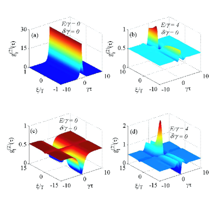
Figure 4: (Color online) The second-order correlation function $g_{r}^{(2)}(\tau)$ and $g_{l}^{(2)}(\tau)$ vs $\xi/\gamma$ and $\gamma\tau$ when (a),(c) $E/\gamma=0$, $\delta=0$ and (b),(d) $E/\gamma=4$, $\delta=0$.

In Fig. 4, we illustrate the second-order correlation function $g_{r}^{(2)}(\tau)$ and $g_{l}^{(2)}(\tau)$ as a function of the scaled parameters $\xi/\gamma$ and $\gamma\tau$. Here, the parameters are chosen to be the same as those in Figs. 2 and 3 for comparison. At the single-photon resonance, i.e., $E/\gamma=0$ and $\delta/\gamma=0$, we can see that, when $\xi/\gamma\neq 0$, $g_{r}^{(2)}(0)>g_{r}^{(2)}(\tau)$ [Fig. 4(a)] and $g_{l}^{(2)}(0)<g_{l}^{(2)}(\tau)$ [Fig. 4(c)], which represent photon bunching in transmission and photon antibunching in reflection, respectively. Interestingly, the $g_{l}^{(2)}(0)$ approaches zero when $\xi/\gamma\gg 1$, which means that the photon blockade phenomenon takes place in the reflection [Fig. 4(c)]. When $\xi/\gamma=0$, the two photons are reflected completely and independently. At the point $\xi/\gamma=0$, $g_{l}^{(2)}(\tau)=1/2$ (for Fock state $|2\rangle$) and $g_{r}^{(2)}(\tau)$ does not make sense.

On the other hand, Figs. 4(b) and 4(d) show that the two-photon resonance ($\xi=E$) will induce the photon statistics transition between bunching and antibunching. For the two-photon transmission, we see $g_{r}^{(2)}(0)>g_{r}^{(2)}(\tau)$ (bunching) in most region of $\xi/\gamma$ and $g_{r}^{(2)}(0)<g_{r}^{(2)}(\tau)$ (antibunching) around the two-photon resonance point $\xi=E$ [Fig. 4(b)]. For comparison, the result for the two-photon reflection is shown in Fig. 4(d). We can see $g_{l}^{(2)}(0)>g_{l}^{(2)}(\tau)$ (bunching) around $\xi=E$ and $g_{l}^{(2)}(0)<g_{l}^{(2)}(\tau)$ (antibunching) in other regions. These results are consistent with our analysis on photon correlation given in Sec. IV(c).

V Conclusion

To conclude, we have studied the transport of photonic wave packets in a 1D waveguide, controlled by the Rydberg interaction between two atoms. We have found that the quantum statistical properties of the scattered photons can be predicted from the relative wave function of the two photons as well as the second-order correlation function. With detailed calculations about the relative wave functions, we have also pointed out how to control the statistics of the scattered photons in the confined system. On one hand, for a certain Rydberg interaction strength, by adjusting the photon-atom detuning, it is possible to control the photon-statistics transition between bunching and antibunching. On the other hand, for a certain total center detuning, we can regulate the Rydberg interaction strength by varying the distance between the two atoms or select two different energy levels of the Rydberg atoms. We can use the change of the quantum statistic properties to detect the detail fashion of the Rydberg interaction between the two atoms.

Appendix A SOLUTION OF EQ. (18) BY THE LAPLACE TRANSFORM

In this appendix, we present a detailed derivation of Eq. (21) by employing the Laplace transform. Under the initial condition (19), the equation of motion (18) becomes

$$s\tilde{A}(s) = -i\xi\tilde{A}(s)-ig\int_{0}^{\infty}dk[\tilde{B}_{k}(s)+\tilde{C}_{k}(s)],$$

$$s\tilde{B}_{k}(s) = -i\Delta_{k}\tilde{B}_{k}(s)-ig\tilde{A}(s)-ig\int_{0}^{\infty}dp\tilde{D}_{p,k}(s),$$

$$s\tilde{C}_{k}(s) = -i\Delta_{k}\tilde{C}_{k}(s)-ig\tilde{A}(s)-ig\int_{0}^{\infty}dp\tilde{D}_{p,k}(s),$$

$$s\tilde{D}_{p,q}(s) = D_{p,q}(0)-i(\Delta_{p}+\Delta_{q})\tilde{D}_{p,q}(s)$$ (52)

$$-ig[\tilde{B}_{p}(s)+\tilde{B}_{q}(s)+\tilde{C}_{p}(s)+\tilde{C}_{q}(s)].$$

By eliminating other variables, we obtain the following equation for the variable $\tilde{B}_{k}(s)$:

$$[\Delta_{k}-i(s+\gamma)]\tilde{B}_{k}(s)$$ (53)

$$= 2g^{2}\int_{-\infty}^{\infty}d\Delta_{p}\left(\frac{1}{\xi-is}+\frac{1}{\Delta_{p}+\Delta_{k}-is}\right)\tilde{B}_{p}(s)$$

$$+ig\int_{-\infty}^{\infty}\frac{D_{p,k}(0)}{\Delta_{p}+\Delta_{k}-is}d\Delta_{p}.$$

The solution of $\tilde{B}_{k}(s)$ can be obtained as

$$\tilde{B}_{k}(s) = \frac{2\pi gG_{2}}{\Delta_{k}-i(s+\gamma)}[\widetilde{f}_{1}+2e^{-sl_{1}}\gamma(\widetilde{f}_{2}+\widetilde{f}_{3})]$$ (54)

$$\times\Theta(l_{1})\Theta(l_{2})\Theta(l_{1}-l_{2}),$$

with

$$\widetilde{f}_{1} = \frac{e^{-sl_{1}}e^{-i\left(l_{1}-l_{2}\right)\Delta_{k}}}{\left(\Delta_{k}-\delta_{2}+i\epsilon\right)\left(\Delta_{k}+\delta_{1}-i\left(s+\epsilon\right)\right)}+\frac{e^{-sl_{2}}e^{i\left(l_{1}-l_{2}\right)\Delta_{k}}}{\left(\Delta_{k}-\delta_{1}+i\epsilon\right)\left(\Delta_{k}+\delta_{2}-i\left(s+\epsilon\right)\right)},$$

$$\widetilde{f}_{2} = \frac{e^{-i\left(l_{1}-l_{2}\right)\Delta_{k}}}{\left(\Delta_{k}+i\gamma\right)\left(\Delta_{k}-\delta_{2}+i\epsilon\right)\left(s+\epsilon+i\left(\Delta_{k}+\delta_{1}\right)\right)}+\frac{e^{-\left(l_{1}-l_{2}\right)\gamma}}{\left(\gamma-\epsilon-i\delta_{2}\right)\left(s+\gamma+\epsilon+i\delta_{1}\right)}\left(\frac{1}{-\gamma+i\Delta_{k}}+\frac{1}{s+\gamma+i\xi}\right),$$

$$\widetilde{f}_{3} = \frac{e^{-\left(l_{1}-l_{2}\right)\left(i\delta_{2}+\epsilon\right)}}{s+i\delta_{1}+i\delta_{2}+2\epsilon}\left(\frac{1}{\left(i\gamma+\delta_{2}-i\epsilon\right)\left(\delta_{2}-\Delta_{k}-i\epsilon\right)}-\frac{1}{\left(s+\gamma+i\delta_{2}+\epsilon\right)\left(s+i\delta_{2}+i\Delta_{k}+\epsilon\right)}\right.$$ (55)

$$\left.-\frac{1}{\left(\gamma-i\delta_{2}-\epsilon\right)\left(s+\gamma+i\xi\right)}-\frac{1}{\left(s+\gamma+i\delta_{2}+\epsilon\right)\left(s+\gamma+i\xi\right)}\right).$$

Then we have

$$\tilde{D}_{p,q}(s)=\frac{D_{p,q}(0)-2ig[\tilde{B}_{p}(s)+\tilde{B}_{q}(s)]}{s+i(\Delta_{p}+\Delta_{q})}.$$ (56)

The transient solution of $D_{p,q}(t)$ can be obtained using the inverse Laplace transform. For studying photon scattering, it is sufficient to get the long-time solution given in Eq. (21).

References

- (1) D. E. Chang, A. S. Sørensen, E. A. Demler, and M. D. Lukin, Nature Phys. 3, 807 (2007).
- (2) J. T. Shen and S. Fan, Opt. Lett. 30, 2001 (2005); Phys. Rev. Lett. 95, 213001 (2005).
- (3) J. T. Shen and S. Fan, Phys. Rev. Lett. 98, 153003 (2007); Phys. Rev. A 76, 062709 (2007).
- (4) L. Zhou, Z. R. Gong, Y. X. Liu, C. P. Sun, and F. Nori, Phys. Rev. Lett. 101, 100501 (2008).
- (5) Z. R. Gong, H. Ian, L. Zhou, and C. P. Sun, Phys. Rev. A. 78, 053806 (2008).
- (6) T. S. Tsoi and C. K. Law, Phys. Rev. A 78, 063832 (2008); 80, 033823 (2009).
- (7) T. Shi and C. P. Sun, Phys. Rev. B 79, 205111 (2009).
- (8) J. Q. Liao, J. F. Huang, Y. X. Liu, L. M. Kuang, and C. P. Sun, Phys. Rev. A 80, 014301 (2009).
- (9) T. Shi and C. P. Sun, e-print arXiv:0907.2776.
- (10) T. S. Tsoi, M. Phil. thesis, The Chinese University of Hong Kong, 2009.
- (11) J. Q. Liao, Z. R. Gong, L. Zhou, Y. X. Liu, C. P. Sun, and F. Nori, Phys. Rev. A 81, 042304 (2010).
- (12) J. Q. Liao and C. K. Law, Phys. Rev. A 82, 053836 (2010).
- (13) D. Z. Xu, H. Ian, T. Shi, H. Dong, and C. P. Sun, Sci. China Phys. Mech. and Astron. 53, 1234 (2010).
- (14) D. Roy, Phys. Rev. B 81, 155117 (2010); Phys. Rev. Lett. 106, 053601 (2011).
- (15) Y. Chang, Z. R. Gong, and C. P. Sun, Phys. Rev. A 83, 013825 (2011).
- (16) E. Rephaeli, Ş. E. Kocabaş, and S. Fan, Phys. Rev. A 84, 063832 (2011).
- (17) H. Zheng, D. J. Gauthier, and H. U. Baranger, Phys. Rev. A 85, 043832 (2012).
- (18) T. Shi and S. Fan, e-print arXiv:1208.1258.
- (19) A. Imamoglu, H. Schmidt, G. Woods, and M. Deutsch, Phys. Rev. Lett. 79, 1467 (1997).
- (20) K. M. Birnbaum, A. Boca, R. Miller, A. D. Boozer, T. E. Northup, and H. J. Kimble, Nature (London) 436, 87 (2005).
- (21) T. Peyronel, O. Firstenberg, Q.-Y. Liang, S. Hofferberth, A. V. Gorshkov, T. Pohl, M. D. Lukin, and V. Vuletić, Nature (London) 488, 57 (2012).
- (22) T. Shi, S. Fan, and C. P. Sun, Phys. Rev. A 84, 063803 (2011).
- (23) D. Jaksch, J. I. Cirac, P. Zoller, S. L. Rolston, R. Côté and M. D. Lukin, Phys. Rev. Lett. 85, 2208 (2000).
- (24) M. D. Lukin, M. Fleischhauer, R. Cote, L. M. Duan, D. Jaksch, J. I. Cirac, and P. Zoller, Phys. Rev. Lett. 87, 037901 (2001).
- (25) D. Tong, S. M. Farooqi, J. Stanojevic, S. Krishnan, Y. P. Zhang, R. Côté, E. E. Eyler, and P. L. Gould, Phys. Rev. Lett. 93, 063001 (2004).
- (26) E. Urban, T. A. Johnson, T. Henage, L. Isenhower, D. D. Yavuz, T. G. Walker, and M. Saffman, Nature Phys. 5, 110 (2009).
- (27) A. Gaëtan, Y. Miroshnychenko, T. Wilk, A. Chotia, M. Viteau, D. Comparat, P. Pillet, A. Browaeys, and P. Grangier, Nature Phys. 5, 115 (2009).
- (28) J. F. Huang, Q. Ai, Y. Deng, C. P. Sun, and F. Nori, Phys. Rev. A 85, 023801 (2012).
- (29) J. D. Pritchard, D. Maxwell, A. Gauguet, K. J. Weatherill, M. P. A. Jones, and C. S. Adams, Phys. Rev. Lett. 105, 193603 (2010).
- (30) J. Honer, R. Löw, H. Weimer, T. Pfau, and H. P. Büchler, Phys. Rev. Lett. 107, 093601 (2011).
- (31) A. V. Gorshkov, J. Otterbach, M. Fleischhauer, T. Pohl, and M. D. Lukin, Phys. Rev. Lett. 107, 133602 (2011).
- (32) J. D. Pritchard, C. S. Adams, and K. Mølmer, Phys. Rev. Lett. 108, 043601 (2012).
- (33) M. Marinescu, Phys. Rev. A 56, 4764 (1997).
- (34) C. Boisseau, I. Simbotin, and R. Côté, Phys. Rev. Lett. 88, 133004 (2002).
- (35) T. Amthor, C. Giese, C. S. Hofmann, and M. Weidemüller, Phys. Rev. Lett. 104, 013001 (2010).
- (36) J. Stanojevic, V. Parigi, E. Bimbard, A. Ourjoumtsev, P. Pillet, and P. Grangier, Phys. Rev. A 86, 021403(R) (2012).
- (37) D. Yan, C. L. Cui, M. Zhang, and J. H. Wu, Phys. Rev. A 84, 043405 (2011).