Discontinuous Galerkin methods for the $p$–biharmonic equation from a discrete variational perspective

Abstract.

We study discontinuous Galerkin approximations of the $p$–biharmonic equation for $p\in(1,\infty)$ from a variational perspective. We propose a discrete variational formulation of the problem based on a appropriate definition of a finite element Hessian and study convergence of the method (without rates) using a weak lower semicontinuity argument. We also present numerical experiments aimed at testing the robustness of the method.

1. Introduction, problem setup and notation

The $p$–biharmonic equation is a fourth order elliptic boundary value problem, related to, in fact a nonlinear generalisation of, the biharmonic problem. Such problems typically arise from areas of elasticity, in particular the nonlinear case can be used as a model for travelling waves in suspension bridges [LM90, GM10]. It is a fourth order analog to its second order sibling, the $p$–Laplacian, and, as such, is useful as a prototypical nonlinear fourth order problem.

The efficient numerical simulation of general fourth order problems has attracted recent interest. A conforming approach to this class of problem would require the use of $\operatorname{C}^{1}$ finite elements, the Argyris element for example [Cia78, Section 6]. From a practical point of view the approach presents difficulties, in that the $\operatorname{C}^{1}$ finite elements are difficult to design and complicated to implement, especially when working in three spatial dimensions.

Discontinuous Galerkin (dG) methods form a class of nonconforming finite element method. They are extremely popular due to their successful application to an ever expanding range of problems. A very accessible unification of these methods together with a detailed historical overview is presented in [ABCM02].

If $p=2$ we have the special case that the ($2$–)biharmonic problem is linear. It has been well studied in the context of dG methods, for example, the papers [LS03, GH09] study the use of $h$–$p$ dG finite elements (where $p$ here means the local polynomial degree) applied to the ($2$–)biharmonic problem. To the authors knowledge there is currently no finite element method posed for the general $p$–biharmonic problem.

In this work we use discrete variational techniques to build a discontinuous Galerkin (dG) numerical scheme for the $p$–biharmonic operator with $p\in(1,\infty)$ . We are interested in such a methodology due to the applications to discrete symmetries, in particular, discrete versions of Noether’s Theorem [Noe71].

A key constituent to the numerical method for the $p$–biharmonic problem (and second order variational problems in general) is an appropriate definition of the Hessian of a piecewise smooth function. To formulate the general dG scheme for this problem from a variational perspective one must construct an appropriate notion of a Hessian of a piecewise smooth function. The finite element Hessian was first coined by [AM09] for use in the characterisation of discrete convex functions. Later in [LP11] it was used in a method for nonvariational problems where the strong form of the PDE was approximated and put to use in the context of fully nonlinear problems in [LP13].

Convergence of the method we propose is proved using the framework set out in [DPE10] where some extremely useful discrete functional analysis results are given. Here, the authors use the framework to prove convergence for a dG approximation to the steady state incompressible Navier–Stokes equations. A related but independent work containing similar results is given in [BO09] where the authors study dG approximations to generic first order variational minimisation problems.

The rest of the paper is set out as follows: The rest of this section introduces necessary notation and the model problem we consider. In Section 2 we give some properties of the continuous $p$–biharmonic problem. In Section 3 we give the methodology for discretisation of the model problem. In Section 4 we detail solvability and the convergence of the discrete problem. Finally, in Section 5 we study the discrete problem computationally and summarise numerical experiments.

Let $\Omega\subset\mathbb{R}^{d}$ be a bounded domain with boundary $\partial\Omega$. We begin by introducing the Sobolev spaces [Cia78, Eva98]

(1.1) $$\operatorname{L}_{p}(\Omega)=\left\{\phi:\;\int_{\Omega}\left|\phi\right|^{p}<\infty\right\}\text{ for }p\in[1,\infty)\text{ and }\operatorname{L}_{\infty}(\Omega)=\left\{\phi:\;\operatorname{ess\,sup}_{\Omega}\left|\phi\right|<\infty\right\},$$

(1.2) $$\operatorname{W}^{l}_{p}(\Omega)=\left\{\phi\in\operatorname{L}_{p}(\Omega):\;\mathrm{D}^{\boldsymbol{\mathsf{\alpha}}}\phi\in\operatorname{L}_{p}(\Omega),\text{ for }\left|\boldsymbol{\alpha}\right|\leq l\right\}\text{ and }\operatorname{H}^{l}(\Omega):=\operatorname{W}^{l}_{2}(\Omega),$$

which are equipped with the following norms and semi-norms:

(1.3) $$\left\|v\right\|_{\operatorname{L}_{p}(\Omega)}^{p}:={\int_{\Omega}\left|v\right|^{p}}$$

(1.4) $$\left\|v\right\|_{l,p}^{p}:=\left\|v\right\|_{\operatorname{W}^{l}_{p}(\Omega)}^{p}=\sum_{\left|\boldsymbol{\mathsf{\alpha}}\right|\leq k}\left\|\mathrm{D}^{\boldsymbol{\mathsf{\alpha}}}v\right\|_{\operatorname{L}_{p}(\Omega)}^{p}$$

(1.5) $$\left|v\right|_{l,p}^{p}:=\left|v\right|_{\operatorname{W}^{l}_{p}(\Omega)}^{p}=\sum_{\left|\boldsymbol{\mathsf{\alpha}}\right|=k}\left\|\mathrm{D}^{\boldsymbol{\mathsf{\alpha}}}v\right\|_{\operatorname{L}_{p}(\Omega)}^{p}$$

(1.6) $$\left\|v\right\|_{l}^{2}:=\left\|v\right\|_{\operatorname{H}^{l}(\Omega)}^{2}=\left\|v\right\|_{\operatorname{W}^{l}_{2}(\Omega)}^{2},$$

where $\boldsymbol{\mathsf{\alpha}}=\{\alpha_{1},\dots,\alpha_{d}\}$ is a multi-index, $\left|\boldsymbol{\mathsf{\alpha}}\right|=\sum_{i=1}^{d}\alpha_{i}$ and derivatives $\mathrm{D}^{\boldsymbol{\mathsf{\alpha}}}$ are understood in a weak sense. We pay particular attention to the cases $l=1,2$ and

(1.7) $${\overset{\smash{\scriptscriptstyle\circ}}{\operatorname{W}}}{}^{2}_{p}(\Omega):=\left\{\phi\in\operatorname{W}^{2}_{p}(\Omega):\;\phi={\!\left({\nabla\phi}\right)}^{{\boldsymbol{\intercal}}}\boldsymbol{n}=0\right\}.$$

In this paper we use the convention that the derivative $\mathrm{D}u$ of a function $u:\Omega\to\mathbb{R}$ is a row vector, while the gradient of $u$, $\nabla u$ is the derivatives transpose, i.e., $\nabla u={\left(\mathrm{D}u\right)}^{{\boldsymbol{\intercal}}}$. We will make use of the slight abuse of notation, following a common practice, whereby the Hessian of $u$ is denoted as $\mathrm{D}^{2}u$ (instead of the correct $\nabla\mathrm{D}u$) and is represented by a $d\times d$ matrix.

Let $L=L\!\left({\boldsymbol{x},u,\nabla u,\mathrm{D}^{2}u}\right)$ be the Lagrangian. We will let

(1.8) $$\begin{array}[]{rccl}{\mathscr{J}[\ \cdot\ ;p]}:&{{\overset{\smash{\scriptscriptstyle\circ}}{\operatorname{W}}}{}^{2}_{p}(\Omega)}&\to&{\mathbb{R}}\\ &{\phi}&\mapsto&{\mathscr{J}[\phi;p]:=\int_{\Omega}L(\boldsymbol{x},\phi,\nabla\phi,\mathrm{D}^{2}\phi)\,\mathrm{d}\boldsymbol{x}}\end{array}\quad$$

be known as the action functional. For the $p$–biharmonic problem the action functional is given explicitly as

(1.9) $$\mathscr{J}[u;p]:=\int_{\Omega}L(\boldsymbol{x},u,\nabla u,\mathrm{D}^{2}u)=\int_{\Omega}\frac{1}{p}\left|\Delta u\right|^{p}-fu,$$

where $\Delta u:=\operatorname{trace}\!\left({\mathrm{D}^{2}u}\right)$ is the Laplacian and $f\in\operatorname{L}_{q}(\Omega)$ is a known source function. We then look to find a minimiser over the space ${\overset{\smash{\scriptscriptstyle\circ}}{\operatorname{W}}}{}^{2}_{p}(\Omega)$, that is, to find $u\in{\overset{\smash{\scriptscriptstyle\circ}}{\operatorname{W}}}{}^{2}_{p}(\Omega)$ such that

(1.10) $$\mathscr{J}[u;p]=\min_{v\in{\overset{\smash{\scriptscriptstyle\circ}}{\operatorname{W}}}{}^{2}_{p}(\Omega)}\mathscr{J}[v;p].$$

If we assume temporarily that we have access to a smooth minimiser, i.e., $u\in\operatorname{C}^{4}(\Omega)$, then, given that the Lagrangian is of second order, we have that the Euler–Lagrange equations are (in general) fourth order.

Let ${\boldsymbol{X}}{:}{\boldsymbol{Y}}=\operatorname{trace}\!\left({{\boldsymbol{X}}^{{\boldsymbol{\intercal}}}\boldsymbol{Y}}\right)$ be the Frobenious inner product between matrices. We then let

(1.11) $$\boldsymbol{X}=\begin{bmatrix}{{x}}_{1}^{1}&\dotsc&{{x}}_{1}^{d}\\ \vdots&\ddots&\vdots\\ {{x}}_{d}^{1}&\dotsc&{{x}}_{d}^{d}\end{bmatrix}$$

then use

(1.12) $${\frac{\partial L}{\partial\!\left({\boldsymbol{X}}\right)}}:=\begin{bmatrix}{{{\partial L}/{\partial{x}}}}_{1}^{1}&\dotsc&{{{\partial L}/{\partial{x}}}}_{1}^{d}\\ \vdots&\ddots&\vdots\\ {{{\partial L}/{\partial{x}}}}_{d}^{1}&\dotsc&{{{\partial L}/{\partial{x}}}}_{d}^{d}\end{bmatrix}.$$

The Euler–Lagrange equations for this problem then take the following form:

(1.13) $$\mathscr{L}[u;p]:={\mathrm{D}^{2}}{:}{\!\left({\frac{\partial L}{\partial\!\left({\mathrm{D}^{2}u}\right)}}\right)}+\frac{\partial L}{\partial u}=0.$$

These can then be calculated to be

(1.14) $$\mathscr{L}[u;p]:=\Delta\!\left({\left|\Delta u\right|^{p-2}\Delta u}\right)-f=0.$$

Note that, for $p=2$, the problem coincides with the biharmonic problem $\Delta^{2}u=f$ which is well studied in the context of dG methods [Bak77, SM07, GNP08, GH09, e.g.].

2. Properties of the continuous problem

To the authors knowledge the numerical method presented here is the first finite element method presented for the $p$–biharmonic problem. As such, we will state some simple properties of the problem which are well known for the problem’s second order counterpart the $p$–Laplacian [Cia78, BE08].

2.1 Proposition (equivalence of norms over ${\overset{\smash{\scriptscriptstyle\circ}}{\operatorname{W}}}{}^{2}_{p}(\Omega)$ [GT83, Cor 9.10]).

Let $\Omega$ be a bounded domain with Lipschitz boundary then the norms $\left\|\cdot\right\|_{2,p}$ and $\left\|\mathrm{D}^{2}\cdot\right\|_{\operatorname{L}_{p}(\Omega)}$ are equivalent over ${\overset{\smash{\scriptscriptstyle\circ}}{\operatorname{W}}}{}^{2}_{p}(\Omega)$.

2.2 Proposition (coercivity of $\mathscr{J}$).

Let $u\in{\overset{\smash{\scriptscriptstyle\circ}}{\operatorname{W}}}{}^{2}_{p}(\Omega)$ and $f\in\operatorname{L}_{q}(\Omega)$, where $\tfrac{1}{p}+\tfrac{1}{q}=1$, we have that the action functional $\mathscr{J}[\ \cdot\ ;p]$ is coercive over ${\overset{\smash{\scriptscriptstyle\circ}}{\operatorname{W}}}{}^{2}_{p}(\Omega)$, that is,

(2.1) $$\mathscr{J}[u;p]\geq C\left|u\right|^{p}_{2,p}-\gamma,$$

for some $C>0\text{ and }\gamma\geq 0$. Equivalently, let

(2.2) $$\mathscr{A}\!\left({u,v;p}\right)=\int_{\Omega}\left|\Delta u\right|^{p-2}\Delta u\Delta v$$

then we have that there exists a constant $C>0$ such that

(2.3) $$\mathscr{A}\!\left({v,v;p}\right)\geq C\left|v\right|_{2,p}^{p}\quad\>\forall\>v\in{\overset{\smash{\scriptscriptstyle\circ}}{\operatorname{W}}}{}^{2}_{p}(\Omega).$$

Proof By definition of the ${\overset{\smash{\scriptscriptstyle\circ}}{\operatorname{W}}}{}^{2}_{p}(\Omega)$ norm and Proposition 2.1 we have that

(2.4) $$\mathscr{J}[u;p]\geq C(p)\left|u\right|_{2,p}^{p}-fu.$$

Upon applying Hölder and Poincaré–Friedrichs inequalities we see

(2.5) $$\begin{split}\mathscr{J}[u;p]&\geq C(p)\left|u\right|_{2,p}^{p}-\left\|f\right\|_{\operatorname{L}_{q}(\Omega)}\left\|u\right\|_{\operatorname{L}_{p}(\Omega)}\\ &\geq C(p)\left|u\right|_{2,p}^{p}-C\left\|f\right\|_{\operatorname{L}_{q}(\Omega)}.\end{split}$$

The statement (2.3) is clear due to Proposition 2.1, thus concluding the proof. ∎

2.3 Proposition (convexity of $L$).

The Lagrangian of the $p$–biharmonic problem is convex with respect to its fourth argument.

Proof Using similar arguments to [Cia78, Section 5.3] (also found in [BL94]) the convexity of the functional $J$ is a consequence of the convexity of the mapping

(2.6) $$\mathscr{F}:\xi\in\mathbb{R}\to\frac{1}{p}\left\|\xi\right\|^{p}.$$

∎

2.4 Corollary (weak lower semicontinuity).

The action functional $\mathscr{J}$ is weakly lower semicontinuous over ${\overset{\smash{\scriptscriptstyle\circ}}{\operatorname{W}}}{}^{2}_{p}(\Omega)$. That is, given a sequence of functions $\{u_{j}\}_{j\in\mathbb{N}}$ who has a weak limit $u\in{\overset{\smash{\scriptscriptstyle\circ}}{\operatorname{W}}}{}^{2}_{p}(\Omega)$, then

(2.7) $$\mathscr{J}[u;p]\leq\liminf_{j\to\infty}\mathscr{J}[u_{j};p].$$

Proof The proof of this is a straightforward extension of [Eva98, Section 8.2 Thm 1] to second order Lagrangians, noting that $\mathscr{J}$ is coercive (from Proposition 2.2) and that $L$ is convex with respect to its fourth variable (from Proposition 2.3). We omit the full details for brevity. ∎

2.5 Corollary (existence and uniquness).

There exists a unique minimiser to the $p$–biharmonic equation. Equivalently there is a unique (weak) solution to the (weak) Euler–Lagrange equations, find $u\in{\overset{\smash{\scriptscriptstyle\circ}}{\operatorname{W}}}{}^{2}_{p}(\Omega)$ such that

(2.8) $$\int_{\Omega}\left|\Delta u\right|^{p-2}\Delta u\Delta\phi=\int_{\Omega}f\phi\quad\>\forall\>\phi\in{\overset{\smash{\scriptscriptstyle\circ}}{\operatorname{W}}}{}^{2}_{p}(\Omega).$$

Proof Again, the result can be deduced by extending the arguments in [Eva98, Section 8.2] or [Cia78, Thm 5.3.1], again, noting the results of Propositions 2.2 and 2.3. The full argument is omitted for brevity. ∎

3. Discretisation

Let $\mathscr{T}$ be a conforming, shape regular triangulation of $\Omega$, namely, $\mathscr{T}$ is a finite family of sets such that

1. $K\in\mathscr{T}$ implies $K$ is an open simplex (segment for $d=1$, triangle for $d=2$, tetrahedron for $d=3$),

2. for any $K,J\in\mathscr{T}$ we have that $\overline{K}\cap\overline{J}$ is a full subsimplex (i.e., it is either $\emptyset$, a vertex, an edge, a face, or the whole of $\overline{K}$ and $\overline{J}$) of both $\overline{K}$ and $\overline{J}$ and

3. $\bigcup_{K\in\mathscr{T}}\overline{K}=\overline{\Omega}$.

The shape regularity of $\mathscr{T}$ is defined as the number

(3.1) $$\mu(\mathscr{T}):=\inf_{K\in\mathscr{T}}\frac{\rho_{K}}{h_{K}},$$

where $\rho_{K}$ is the radius of the largest ball contained inside $K$ and $h_{K}$ is the diameter of $K$. An indexed family of triangulations $\left\{{\mathscr{T}^{n}}\right\}_{n}$ is called shape regular if

(3.2) $$\mu:=\inf_{n}\mu(\mathscr{T}^{n})>0.$$

We use the convention where $h:\Omega\to\mathbb{R}$ denotes the piecewise constant meshsize function of $\mathscr{T}$, i.e.,

(3.3) $$h(\boldsymbol{x}):=\max_{\overline{K}\ni\boldsymbol{x}}h_{K},$$

which we shall commonly refer to as $h$.

We let $\mathscr{E}{}$ be the skeleton (set of common interfaces) of the triangulation $\mathscr{T}$ and say $e\in\mathscr{E}$ if $e$ is on the interior of $\Omega$ and $e\in\partial\Omega$ if $e$ lies on the boundary $\partial\Omega$ and set $h_{e}$ to be the diameter of $e$.

We also make the assumption that the mesh is sufficiently shape regular such that for any $K\in\mathscr{T}$ we have the existence of a constant such that

(3.4) $$\sum_{e\in\partial K}h_{e}\left|e\right|\leq C\left|K\right|,$$

where $\left|e\right|$ and $\left|K\right|$ denote the $d-1$ and $d$ dimensional measure of $e$ and $K$ respectively.

We let $\mathbb{P}^{k}(\mathscr{T})$ denote the space of piecewise polynomials of degree $k$ over the triangulation $\mathscr{T}$,i.e.,

(3.5) $$\mathbb{P}^{k}(\mathscr{T})=\{\phi\text{ such that }\phi|_{K}\in\mathbb{P}^{k}(K)\}$$

and introduce the finite element space

(3.6) $$\mathbb{V}:=\mathbb{D}\mathbb{G}({\mathscr{T}},{k})=\mathbb{P}^{k}(\mathscr{T})$$

to be the usual space of discontinuous piecewise polynomial functions.

3.1 Definition (finite element sequence).

A finite element sequence $\{v_{h},\mathbb{V}\}$ is a sequence of discrete objects, indexed by the mesh parameter $h$, individually represented on a particular finite element space, $\mathbb{V}$, which itself has discretisation parameter $h$, that is, we have that $\mathbb{V}=\mathbb{V}(h)$.

3.2 Definition (broken Sobolev spaces, trace spaces).

We introduce the broken Sobolev space

(3.7) $$\operatorname{W}^{l}_{p}(\mathscr{T}):=\left\{\phi:\;\phi|_{K}\in\operatorname{W}^{l}_{p}(K),\text{ for each }K\in\mathscr{T}\right\}.$$

We also make use of functions defined in these broken spaces restricted to the skeleton of the triangulation. This requires an appropriate trace space

(3.8) $$\mathcal{T}\!\left({\mathscr{E}}\right):=\prod_{K\in\mathscr{T}}\operatorname{L}_{2}(\partial K){\supset}\prod_{K\in\mathscr{T}}\operatorname{W}^{l-\frac{1}{2}}_{p}(K)$$

for $p\geq 2$, $l\geq 1$.

3.3 Definition (jumps, averages and tensor jumps).

We may define average, jump and tensor jump operators over $\mathcal{T}\!\left({\mathscr{E}}\right)$ for arbitrary scalar functions $v\in\mathcal{T}\!\left({\mathscr{E}}\right)$ and vectors $\boldsymbol{v}\in\mathcal{T}\!\left({\mathscr{E}}\right)^{d}$.

(3.9) $$\begin{array}[]{rccl}{\mathrel{\ooalign{\cr\kern 1.0pt$\{$\cr\kern-0.5pt$\{$}}\cdot\mathrel{\ooalign{$\}$\cr\kern-1.5pt$\}$\cr\kern-1.0pt}}}:&{\mathcal{T}\!\left({\mathscr{E}\cup\partial\Omega}\right)}&\to&{\operatorname{L}_{2}(\mathscr{E}\cup\partial\Omega)}\\ &{v}&\mapsto&{\begin{cases}\frac{1}{2}\!\left({v|_{K_{1}}+v|_{K_{2}}}\right)\text{ over }\mathscr{E}\\ v|_{\partial\Omega}\text{ on }\partial\Omega\end{cases}}\end{array}\quad$$

(3.10) $$\begin{array}[]{rccl}{\mathrel{\ooalign{\cr\kern 1.0pt$\{$\cr\kern-0.5pt$\{$}}\cdot\mathrel{\ooalign{$\}$\cr\kern-1.5pt$\}$\cr\kern-1.0pt}}}:&{\!\left[{\mathcal{T}\!\left({\mathscr{E}\cup\partial\Omega}\right)}\right]^{d}}&\to&{\!\left[{\operatorname{L}_{2}(\mathscr{E}\cup\partial\Omega)}\right]^{d}}\\ &{\boldsymbol{v}}&\mapsto&{\begin{cases}\frac{1}{2}\!\left({\boldsymbol{v}|_{K_{1}}+\boldsymbol{v}|_{K_{2}}}\right)\text{ over }\mathscr{E}\\ \boldsymbol{v}|_{\partial\Omega}\text{ on }\partial\Omega\end{cases}}\end{array}\quad$$

(3.11) $$\begin{array}[]{rccl}{\left\llbracket\cdot\right\rrbracket}:&{{\mathcal{T}\!\left({\mathscr{E}\cup\partial\Omega}\right)}}&\to&{\!\left[{\operatorname{L}_{2}(\mathscr{E}\cup\partial\Omega)}\right]^{d}}\\ &{v}&\mapsto&{\begin{cases}{{v}|_{K_{1}}\boldsymbol{n}_{K_{1}}+{v}|_{K_{2}}}\boldsymbol{n}_{K_{2}}\text{ over }\mathscr{E}\\ \!\left({v\boldsymbol{n}}\right)|_{\partial\Omega}\text{ on }\partial\Omega\end{cases}}\end{array}\quad$$

(3.12) $$\begin{array}[]{rccl}{\left\llbracket\cdot\right\rrbracket}:&{\!\left[{\mathcal{T}\!\left({\mathscr{E}\cup\partial\Omega}\right)}\right]^{d}}&\to&{{\operatorname{L}_{2}(\mathscr{E}\cup\partial\Omega)}}\\ &{\boldsymbol{v}}&\mapsto&{\begin{cases}{{\!\left({\boldsymbol{v}|_{K_{1}}}\right)}^{{\boldsymbol{\intercal}}}\boldsymbol{n}_{K_{1}}+{\!\left({\boldsymbol{v}|_{K_{2}}}\right)}^{{\boldsymbol{\intercal}}}\boldsymbol{n}_{K_{2}}}\text{ over }\mathscr{E}\\ \!\left({{\boldsymbol{v}}^{{\boldsymbol{\intercal}}}\boldsymbol{n}}\right)|_{\partial\Omega}\text{ on }\partial\Omega\end{cases}}\end{array}\quad$$

(3.13) $$\begin{array}[]{rccl}{\left\llbracket\cdot\right\rrbracket_{\otimes}}:&{\!\left[{\mathcal{T}\!\left({\mathscr{E}\cup\partial\Omega}\right)}\right]^{d}}&\to&{\!\left[{\operatorname{L}_{2}(\mathscr{E}\cup\partial\Omega)}\right]^{d\times d}}\\ &{\boldsymbol{v}}&\mapsto&{\begin{cases}{\boldsymbol{v}|_{K_{1}}}\otimes\boldsymbol{n}_{K_{1}}+\boldsymbol{v}|_{K_{2}}\otimes\boldsymbol{n}_{K_{2}}\text{ over }\mathscr{E}\\ \!\left({{\boldsymbol{v}}\otimes\boldsymbol{n}}\right)|_{\partial\Omega}\text{ on }\partial\Omega\end{cases}.}\end{array}\quad$$

We will often use the following Proposition which we state in full for clarity but whose proof is merely using the identities in Definition 3.3.

3.4 Proposition (elementwise integration).

For a generic vector valued function $\boldsymbol{p}$ and scalar valued function $\phi$ we have

(3.14) $$\begin{split}\sum_{K\in\mathscr{T}}\int_{K}\operatorname{div}\!\left({\boldsymbol{p}}\right)\phi\,\mathrm{d}\boldsymbol{x}=\sum_{K\in\mathscr{T}}\!\left({-\int_{K}{\boldsymbol{p}}^{{\boldsymbol{\intercal}}}\nabla_{h}\phi\,\mathrm{d}\boldsymbol{x}+\int_{\partial K}\phi{\boldsymbol{p}}^{{\boldsymbol{\intercal}}}\boldsymbol{n}_{K}\,\mathrm{d}s}\right).\end{split}$$

In particular, if we have $\boldsymbol{p}\in\mathcal{T}\!\left({\mathscr{E}\cup\partial\Omega}\right)^{d}$ and $\phi\in\mathcal{T}\!\left({\mathscr{E}\cup\partial\Omega}\right)$, the following identity holds

(3.15) $$\sum_{K\in\mathscr{T}}\int_{\partial K}\phi{{\boldsymbol{p}}}^{{\boldsymbol{\intercal}}}\boldsymbol{n}_{K}\,\mathrm{d}s=\int_{\mathscr{E}}\left\llbracket\boldsymbol{p}\right\rrbracket\mathrel{\ooalign{\cr\kern 1.0pt$\{$\cr\kern-0.5pt$\{$}}\phi\mathrel{\ooalign{$\}$\cr\kern-1.5pt$\}$\cr\kern-1.0pt}}\,\mathrm{d}s+\int_{\mathscr{E}\cup\partial\Omega}{\left\llbracket\phi\right\rrbracket}^{{\boldsymbol{\intercal}}}\mathrel{\ooalign{\cr\kern 1.0pt$\{$\cr\kern-0.5pt$\{$}}\boldsymbol{p}\mathrel{\ooalign{$\}$\cr\kern-1.5pt$\}$\cr\kern-1.0pt}}\,\mathrm{d}s=\int_{\mathscr{E}\cup\partial\Omega}\left\llbracket\boldsymbol{p}\phi\right\rrbracket\,\mathrm{d}s.$$

An equivalent tensor formulation of (3.14)–(3.15) is

(3.16) $$\begin{split}\sum_{K\in\mathscr{T}}\int_{K}\mathrm{D}_{h}{\boldsymbol{p}}\phi\,\mathrm{d}\boldsymbol{x}=\sum_{K\in\mathscr{T}}\!\left({-\int_{K}{\boldsymbol{p}}\otimes\nabla_{h}\phi\,\mathrm{d}\boldsymbol{x}+\int_{\partial K}\phi{\boldsymbol{p}}\otimes\boldsymbol{n}_{K}\,\mathrm{d}s}\right).\end{split}$$

In particular the following identity holds

(3.17) $$\sum_{K\in\mathscr{T}}\int_{\partial K}\phi{\boldsymbol{p}}\otimes\boldsymbol{n}_{K}\,\mathrm{d}s=\int_{\mathscr{E}}\left\llbracket\boldsymbol{p}\right\rrbracket_{\otimes}\mathrel{\ooalign{\cr\kern 1.0pt$\{$\cr\kern-0.5pt$\{$}}\phi\mathrel{\ooalign{$\}$\cr\kern-1.5pt$\}$\cr\kern-1.0pt}}\,\mathrm{d}s+\int_{\mathscr{E}\cup\partial\Omega}{\left\llbracket\phi\right\rrbracket}\otimes\mathrel{\ooalign{\cr\kern 1.0pt$\{$\cr\kern-0.5pt$\{$}}\boldsymbol{p}\mathrel{\ooalign{$\}$\cr\kern-1.5pt$\}$\cr\kern-1.0pt}}\,\mathrm{d}s=\int_{\mathscr{E}\cup\partial\Omega}\left\llbracket\boldsymbol{p}\phi\right\rrbracket_{\otimes}\,\mathrm{d}s.$$

The discrete problem we then propose is to minimise an appropriate discrete action functional, that is to seek $u_{h}\in\mathbb{V}$ such that

(3.18) $$\mathscr{J}_{h}[u_{h};p]=\inf_{v_{h}\in\mathbb{V}}\mathscr{J}_{h}[v_{h};p].$$

3.5 Remark (motivation for discrete action functional).

The choice of discrete action functional is crucial. A naive choice would be to take the piecewise gradient and Hessian operators, substituting them directly into the Lagrangian, i.e.,

(3.19) $$\mathscr{J}_{h}[u_{h};p]=\int_{\Omega}L\!\left({\boldsymbol{x},u_{h},\nabla_{h}u_{h},\mathrm{D}^{2}_{h}u_{h}}\right).$$

This is, however, an inconsistent notion of the derivative operators (as noted in [BO09]).

Since for the biharmonic problem the Lagrangian is only dependant on the Hessian of the sought function, we need only construct an appropriate consistent notion of discrete Hessian.

3.6 Theorem (dG Hessian).

Let $v\in{\overset{\smash{\scriptscriptstyle\circ}}{\operatorname{W}}}{}^{2}_{p}(\mathscr{T})$, $\widehat{v}:\operatorname{H}^{1}(\mathscr{T})\to\mathcal{T}\!\left({\mathscr{E}\cup\partial\Omega}\right)$ be a linear form and $\widehat{\boldsymbol{p}}:\operatorname{H}^{2}(\mathscr{T})\times\operatorname{H}^{1}(\mathscr{T})^{d}\to\mathcal{T}\!\left({\mathscr{E}\cup\partial\Omega}\right)^{d}$ a bilinear form representing consistent numerical fluxes, i.e.,

(3.20) $$\widehat{v}\!\left({v}\right)=v|_{\mathscr{E}\cup\partial\Omega}\qquad\widehat{p}(v,\nabla v)=\nabla v|_{\mathscr{E}\cup\partial\Omega},$$

in the spirit of [ABCM02]. Then the we define the dG Hessian, $\boldsymbol{H}[v]\in\mathbb{V}^{d\times d}$, to be the $\operatorname{L}_{2}$ Reisz representor of the distributional Hessian of $v$. This has the general form

(3.21) $$\begin{split}\int_{\Omega}\boldsymbol{H}[v]\ \Phi&=-\int_{\Omega}\nabla_{h}v\otimes\nabla_{h}\Phi-\int_{\mathscr{E}\cup\partial\Omega}\left\llbracket\widehat{v}-v\right\rrbracket\otimes\mathrel{\ooalign{\cr\kern 1.0pt$\{$\cr\kern-0.5pt$\{$}}\nabla_{h}\Phi\mathrel{\ooalign{$\}$\cr\kern-1.5pt$\}$\cr\kern-1.0pt}}\\ &\qquad-\int_{\mathscr{E}}\mathrel{\ooalign{\cr\kern 1.0pt$\{$\cr\kern-0.5pt$\{$}}\widehat{v}-v\mathrel{\ooalign{$\}$\cr\kern-1.5pt$\}$\cr\kern-1.0pt}}\left\llbracket\nabla_{h}\Phi\right\rrbracket_{\otimes}+\int_{\mathscr{E}\cup\partial\Omega}\left\llbracket\Phi\right\rrbracket\otimes\mathrel{\ooalign{\cr\kern 1.0pt$\{$\cr\kern-0.5pt$\{$}}\boldsymbol{\widehat{p}}\mathrel{\ooalign{$\}$\cr\kern-1.5pt$\}$\cr\kern-1.0pt}}+\int_{\mathscr{E}}\mathrel{\ooalign{\cr\kern 1.0pt$\{$\cr\kern-0.5pt$\{$}}\Phi\mathrel{\ooalign{$\}$\cr\kern-1.5pt$\}$\cr\kern-1.0pt}}\left\llbracket\boldsymbol{\widehat{p}}\right\rrbracket_{\otimes}\\ &\qquad\qquad\quad\>\forall\>\Phi\in\mathbb{V}.\end{split}$$

Proof Note that, in view of Green’s Theorem, for smooth functions, $w\in\operatorname{C}^{2}(\Omega)\cap\operatorname{C}^{1}(\overline{\Omega})$, we have

(3.22) $$\int_{\Omega}\mathrm{D}^{2}w\phi=-\int_{\Omega}\nabla w\otimes\nabla\phi+\int_{\partial\Omega}\nabla w\otimes\boldsymbol{n}\phi\quad\>\forall\>\phi\in\operatorname{C}^{1}(\Omega)\cap\operatorname{C}^{0}(\overline{\Omega}).$$

As such for a broken function $v\in{\overset{\smash{\scriptscriptstyle\circ}}{\operatorname{W}}}{}^{2}_{p}(\mathscr{T})$ we introduce an auxiliary variable $\boldsymbol{p}=\nabla_{h}v$ and consider the following primal form for the representation of the Hessian of said function: For each $K\in\mathscr{T}$

(3.23) $$\int_{K}{\boldsymbol{H}[v]}\ {\Phi}=-\int_{K}\boldsymbol{p}\otimes\nabla_{h}\Phi+\int_{\partial K}\boldsymbol{\widehat{p}}\otimes\boldsymbol{n}\ \Phi\quad\>\forall\>\Phi\in\mathbb{V}$$

(3.24) $$\int_{K}\boldsymbol{p}\otimes\boldsymbol{q}=-\int_{K}v\ \mathrm{D}\boldsymbol{q}+\int_{\partial K}\boldsymbol{q}\otimes\boldsymbol{n}\ \widehat{v}\quad\>\forall\>\boldsymbol{q}\in\mathbb{V}^{d},$$

where $\nabla_{h}={\!\left({\mathrm{D}_{h}}\right)}^{{\boldsymbol{\intercal}}}$ is the elementwise spatial gradient.

Noting the identity (3.17) and taking the sum of (3.23) over $K\in\mathscr{T}$ we see

(3.25) $$\begin{split}\int_{\Omega}{\boldsymbol{H}[v]}\ {\Phi}&=\sum_{K\in\mathscr{T}}\int_{K}{\boldsymbol{H}[v]}\ {\Phi}=\sum_{K\in\mathscr{T}}\!\left({-\int_{K}\boldsymbol{p}\otimes\nabla_{h}\Phi+\int_{\partial K}\boldsymbol{\widehat{p}}\otimes\boldsymbol{n}\ \Phi}\right)\\ &=-\int_{\Omega}\boldsymbol{p}\otimes\nabla_{h}\Phi+\int_{\mathscr{E}\cup\partial\Omega}\left\llbracket\Phi\right\rrbracket\otimes\mathrel{\ooalign{\cr\kern 1.0pt$\{$\cr\kern-0.5pt$\{$}}\boldsymbol{\widehat{p}}\mathrel{\ooalign{$\}$\cr\kern-1.5pt$\}$\cr\kern-1.0pt}}+\int_{\mathscr{E}}\mathrel{\ooalign{\cr\kern 1.0pt$\{$\cr\kern-0.5pt$\{$}}\Phi\mathrel{\ooalign{$\}$\cr\kern-1.5pt$\}$\cr\kern-1.0pt}}\left\llbracket\boldsymbol{\widehat{p}}\right\rrbracket_{\otimes}\end{split}$$

Using the same argument for (3.24)

(3.26) $$\begin{split}\int_{\Omega}\boldsymbol{p}\otimes\boldsymbol{q}&=\sum_{K\in\mathscr{T}}\int_{K}\boldsymbol{p}\otimes\boldsymbol{q}=\sum_{K\in\mathscr{T}}\!\left({-\int_{K}v\ \mathrm{D}_{h}\boldsymbol{q}+\int_{\partial K}\boldsymbol{q}\otimes\boldsymbol{n}\ \widehat{v}}\right)\\ &=-\int_{\Omega}v\ \mathrm{D}_{h}\boldsymbol{q}+\int_{\mathscr{E}\cup\partial\Omega}\left\llbracket\widehat{v}\right\rrbracket\otimes\mathrel{\ooalign{\cr\kern 1.0pt$\{$\cr\kern-0.5pt$\{$}}\boldsymbol{q}\mathrel{\ooalign{$\}$\cr\kern-1.5pt$\}$\cr\kern-1.0pt}}+\int_{\mathscr{E}}\mathrel{\ooalign{\cr\kern 1.0pt$\{$\cr\kern-0.5pt$\{$}}\widehat{v}\mathrel{\ooalign{$\}$\cr\kern-1.5pt$\}$\cr\kern-1.0pt}}\left\llbracket\boldsymbol{q}\right\rrbracket_{\otimes}\end{split}$$

Note that, again making use of (3.17) we have for each $\boldsymbol{q}\in\operatorname{H}^{1}(\mathscr{T})^{d}$ and $w\in\operatorname{H}^{1}(\mathscr{T})$ that

(3.27) $$\int_{\Omega}\boldsymbol{q}\otimes\nabla_{h}w=-\int_{\Omega}\mathrm{D}_{h}\boldsymbol{q}w+\int_{\mathscr{E}\cup\partial\Omega}\mathrel{\ooalign{\cr\kern 1.0pt$\{$\cr\kern-0.5pt$\{$}}\boldsymbol{q}\mathrel{\ooalign{$\}$\cr\kern-1.5pt$\}$\cr\kern-1.0pt}}\otimes\left\llbracket w\right\rrbracket+\int_{\mathscr{E}}\left\llbracket\boldsymbol{q}\right\rrbracket_{\otimes}\mathrel{\ooalign{\cr\kern 1.0pt$\{$\cr\kern-0.5pt$\{$}}w\mathrel{\ooalign{$\}$\cr\kern-1.5pt$\}$\cr\kern-1.0pt}}.$$

Taking $w=v$ in (3.27) and substituting into (3.24) we see

(3.28) $$\int_{\Omega}\boldsymbol{p}\otimes\boldsymbol{q}=\int_{\Omega}\boldsymbol{q}\otimes\nabla_{h}v+\int_{\mathscr{E}\cup\partial\Omega}\left\llbracket\widehat{v}-v\right\rrbracket\otimes\mathrel{\ooalign{\cr\kern 1.0pt$\{$\cr\kern-0.5pt$\{$}}\boldsymbol{q}\mathrel{\ooalign{$\}$\cr\kern-1.5pt$\}$\cr\kern-1.0pt}}+\int_{\mathscr{E}}\mathrel{\ooalign{\cr\kern 1.0pt$\{$\cr\kern-0.5pt$\{$}}\widehat{v}-v\mathrel{\ooalign{$\}$\cr\kern-1.5pt$\}$\cr\kern-1.0pt}}\left\llbracket\boldsymbol{q}\right\rrbracket_{\otimes}.$$

Now choosing $\boldsymbol{q}=\nabla_{h}\Phi$ and substituting (3.28) into (3.23) concludes the proof. ∎

3.7 Example.

An example of the possible choices of fluxes are

(3.29) $$\widehat{v}=\begin{cases}\mathrel{\ooalign{\cr\kern 1.0pt$\{$\cr\kern-0.5pt$\{$}}v\mathrel{\ooalign{$\}$\cr\kern-1.5pt$\}$\cr\kern-1.0pt}}\text{ over }\mathscr{E}\\ 0\text{ on }\partial\Omega\end{cases}$$

(3.36) $$\widehat{\boldsymbol{p}}=\mathrel{\ooalign{\cr\kern 1.0pt$\{$\cr\kern-0.5pt$\{$}}\nabla_{h}v\mathrel{\ooalign{$\}$\cr\kern-1.5pt$\}$\cr\kern-1.0pt}}\text{ on }\mathscr{E}\cup\partial\Omega.$$

The result is an interior penalty (IP) type method [DD76] applied to represent the finite element Hessian

(3.37) $$\begin{split}\int_{\Omega}\boldsymbol{H}[v]\ \Phi&=-\int_{\Omega}\nabla_{h}v\otimes\nabla_{h}\Phi+\int_{\mathscr{E}\cup\partial\Omega}\left\llbracket v\right\rrbracket\otimes\mathrel{\ooalign{\cr\kern 1.0pt$\{$\cr\kern-0.5pt$\{$}}\nabla_{h}\Phi\mathrel{\ooalign{$\}$\cr\kern-1.5pt$\}$\cr\kern-1.0pt}}\\ &\qquad+\int_{\mathscr{E}\cup\partial\Omega}\left\llbracket\Phi\right\rrbracket\otimes\mathrel{\ooalign{\cr\kern 1.0pt$\{$\cr\kern-0.5pt$\{$}}\nabla_{h}v\mathrel{\ooalign{$\}$\cr\kern-1.5pt$\}$\cr\kern-1.0pt}}.\\ &=\int_{\Omega}\mathrm{D}^{2}_{h}v\Phi-\int_{\mathscr{E}\cup\partial\Omega}\left\llbracket\nabla_{h}v\right\rrbracket_{\otimes}\mathrel{\ooalign{\cr\kern 1.0pt$\{$\cr\kern-0.5pt$\{$}}\Phi\mathrel{\ooalign{$\}$\cr\kern-1.5pt$\}$\cr\kern-1.0pt}}\\ &\qquad+\int_{\mathscr{E}\cup\partial\Omega}\left\llbracket v\right\rrbracket\otimes\mathrel{\ooalign{\cr\kern 1.0pt$\{$\cr\kern-0.5pt$\{$}}\nabla_{h}\Phi\mathrel{\ooalign{$\}$\cr\kern-1.5pt$\}$\cr\kern-1.0pt}}.\end{split}$$

This will be the form of the dG Hessian which we will take for the rest of this exposition.

3.8 Definition (lifting operators).

From the IP-Hessian defined in Example 3.7 we define the following lifting operator $l_{1},l_{2}:\mathbb{V}\to\mathbb{V}^{d\times d}$ such that

(3.44) $$\int_{\Omega}l_{1}[v_{h}]\Phi=\int_{\mathscr{E}\cup\partial\Omega}\left\llbracket v_{h}\right\rrbracket\otimes\mathrel{\ooalign{\cr\kern 1.0pt$\{$\cr\kern-0.5pt$\{$}}\nabla_{h}\Phi\mathrel{\ooalign{$\}$\cr\kern-1.5pt$\}$\cr\kern-1.0pt}}$$

(3.51) $$\int_{\Omega}l_{2}[v_{h}]\Phi=-\int_{\mathscr{E}\cup\partial\Omega}\left\llbracket\nabla_{h}u_{h}\right\rrbracket_{\otimes}\mathrel{\ooalign{\cr\kern 1.0pt$\{$\cr\kern-0.5pt$\{$}}\Phi\mathrel{\ooalign{$\}$\cr\kern-1.5pt$\}$\cr\kern-1.0pt}}.$$

As such we may write the IP-Hessian as $\boldsymbol{H}:\mathbb{V}\to\mathbb{V}^{d\times d}$ such that

(3.52) $$\int_{\Omega}\boldsymbol{H}[v_{h}]\Phi=\int_{\Omega}\!\left({\mathrm{D}^{2}_{h}v_{h}+l_{1}[v_{h}]+l_{2}[v_{h}]}\right)\Phi\quad\>\forall\>\Phi\in\mathbb{V},$$

where $\mathrm{D}^{2}_{h}$ denotes the piecewise Hessian operator.

3.9 Remark (relation to the local continuous/discontinuous Galerkin method (LCDG)).

When $\boldsymbol{H}[\cdot]$ restricted to acting on functions in $\mathbb{V}\cap\operatorname{H}^{1}_{0}(\Omega)$ we have that

(3.53) $$\int_{\Omega}\boldsymbol{H}[v_{h}]\Phi=\int_{\Omega}\!\left({\mathrm{D}^{2}v_{h}+l_{2}[v_{h}]}\right)\Phi\quad\>\forall\>\Phi\in\mathbb{V}\cap\operatorname{H}^{1}_{0}(\Omega).$$

This definition coincides with the auxilliary variable introduced in [HHH10] for Kirchoff plate problems. In addition it is the auxilliary variable used in [LP11, LP13] for applications to second order nonvariational PDEs and fully nonlinear PDEs.

4. Convergence

In this section we use the discrete operators from Section 3 to build a consistent discrete variational problem and in addition prove convergence. To that end, we being by defining the natural dG norm for the problem.

4.1 Definition (dG norm).

We define the dG norm for this problem as

(4.1) $${\left\|v_{h}\right\|_{dG,{p}}^{p}:=\left\|\mathrm{D}^{2}_{h}v_{h}\right\|^{p}_{\operatorname{L}_{p}(\Omega)}+h{{}_{e}}^{1-p}\left\|\left\llbracket\nabla_{h}v_{h}\right\rrbracket\right\|^{p}_{\operatorname{L}_{p}(\mathscr{E}\cup\partial\Omega)}+h{{}_{e}}^{1-2p}\left\|\left\llbracket v_{h}\right\rrbracket\right\|^{p}_{\operatorname{L}_{p}(\mathscr{E}\cup\partial\Omega)},}$$

where $\left\|\cdot\right\|_{\operatorname{L}_{p}(\mathscr{E}\cup\partial\Omega)}$ is the $d-1$ dimensional $\operatorname{L}_{p}$ norm over $\mathscr{E}\cup\partial\Omega$.

To prove convergence for the $p$-biharmonic equation we modify the arguments given in [DPE10] to our problem. To keep the exposition clear we will, where possible, use the same notation as in [DPE10].

We state some basic propositions, that is, a trace inequality and inverse inequality in $\operatorname{L}_{p}(\Omega)$, the proof of these is readily available in [Cia78, e.g.]. Henceforth in this section and throughout the rest of the paper we will use $C$ to denote an arbitrary positive constant which may depend upon $\mu,p\text{ and }\Omega$ but is independent of $h$.

4.2 Proposition (trace inequality).

Let $v_{h}\in\mathbb{V}$ be a finite element function then for $p\in(1,\infty)$ there exists a constant $C>0$ such that

(4.2) $$\left\|v_{h}\right\|_{\operatorname{L}_{p}({\mathscr{E}\cup\partial\Omega})}\leq Ch^{-1/p}\left\|v_{h}\right\|_{\operatorname{L}_{p}(\Omega)}.$$

4.3 Proposition (inverse inequality).

Let $v_{h}\in\mathbb{V}$ be a finite element function then for $p\in(1,\infty)$ there exists a constant $C>0$ such that

(4.3) $$\left\|\nabla_{h}v_{h}\right\|^{p}_{\operatorname{L}_{p}(\Omega)}\leq Ch^{-p}\left\|v_{h}\right\|^{p}_{\operatorname{L}_{p}(\Omega)}$$

4.4 Lemma (relating $\left\|\cdot\right\|_{dG,{s}}$ and $\left\|\cdot\right\|_{dG,{t}}$ norms).

For two integers $s,t$ such that $1\leq s<t<\infty$ we have that there exists a constant $C>0$ such that

(4.4) $$\left\|v_{h}\right\|_{dG,{s}}\leq C\left\|v_{h}\right\|_{dG,{t}}.$$

Proof The proof follows a similar line to [DPE10, Lem 6.1]. By definition of the $\left\|\cdot\right\|_{dG,{s}}$ norm we have that

(4.5) $$\begin{split}\left\|v_{h}\right\|_{dG,{s}}^{s}&=\int_{\Omega}\left|\mathrm{D}^{2}_{h}v_{h}\right|^{s}+h{{}_{e}}^{1-s}\int_{\mathscr{E}\cup\partial\Omega}\left|\left\llbracket\nabla_{h}v_{h}\right\rrbracket\right|^{s}+h{{}_{e}}^{1-2s}\int_{\mathscr{E}\cup\partial\Omega}\left|\left\llbracket v_{h}\right\rrbracket\right|^{s}.\end{split}$$

Now let us denote $r=\tfrac{t}{s}$ and $q=\tfrac{r}{r-1}$, that is, we have that $\tfrac{1}{r}+\tfrac{1}{q}=1$. Hence we may deduce that

(4.6) $$\begin{split}\left\|v_{h}\right\|_{dG,{s}}^{s}&=\int_{\Omega}\left|\mathrm{D}^{2}_{h}v_{h}\right|^{s}+\int_{\mathscr{E}\cup\partial\Omega}h{{}_{e}}^{{1}/{q}}h{{}_{e}}^{{\!\left({1-t}\right)}/{r}}\left|\left\llbracket\nabla_{h}v_{h}\right\rrbracket\right|^{s}+\int_{\mathscr{E}\cup\partial\Omega}h{{}_{e}}^{1/q}h{{}_{e}}^{\!\left({1-2t}\right)/r}\left|\left\llbracket v_{h}\right\rrbracket\right|^{s}\\ &\leq\!\left({\int_{\Omega}1^{q}}\right)^{1/{q}}\!\left({\int_{\Omega}\left|\mathrm{D}^{2}_{h}v_{h}\right|^{t}}\right)^{1/r}+\!\left({{h_{e}}\int_{\mathscr{E}\cup\partial\Omega}1^{q}}\right)^{1/q}\!\left({\int_{\mathscr{E}\cup\partial\Omega}h{{}_{e}}^{1-t}\left|\left\llbracket\nabla_{h}v_{h}\right\rrbracket\right|^{t}}\right)^{1/r}\\ &\qquad+\!\left({h{{}_{e}}\int_{\mathscr{E}\cup\partial\Omega}1^{q}}\right)^{1/q}\!\left({\int_{\mathscr{E}\cup\partial\Omega}h{{}_{e}}^{1-2t}\left|\left\llbracket v_{h}\right\rrbracket\right|^{t}}\right)^{1/r}\\ &\leq C\left\|v_{h}\right\|_{dG,{t}}^{s}\end{split}$$

where we have used a Hölder inequality together with

(4.7) $$1-s=1-\tfrac{t}{r}=\tfrac{1}{q}+\tfrac{1-t}{r}\text{ and }$$

(4.8) $$1-2s=1-\tfrac{2t}{r}=\tfrac{1}{q}+\tfrac{1-2t}{r},$$

and the shape regularity of $\mathscr{T}$ given in (3.4), concluding the proof. ∎

4.5 Definition (bounded variation).

Let $\mathscr{V}[\cdot]$ denote the variation functional defined as

(4.9) $$\mathscr{V}[u]:=\sup\left\{\int_{\Omega}u\operatorname{div}{\boldsymbol{\phi}}:\;\boldsymbol{\phi}\in[\operatorname{C}^{1}_{0}(\Omega)]^{d},\left\|\boldsymbol{\phi}\right\|_{\operatorname{L}_{\infty}(\Omega)}\leq 1\right\}.$$

The space of bounded variations denoted BV is the space of functions with bounded variation functional,

(4.10) $$BV:=\left\{\phi\in\operatorname{L}_{1}(\Omega):\;\mathscr{V}[\phi]<\infty\right\}.$$

Note that the variation functional defines a norm over $BV$, we set

(4.11) $$\left\|u\right\|_{BV}=\mathscr{V}[u].$$

4.6 Proposition (control of the $\operatorname{L}_{\frac{d}{d-1}}(\Omega)$ norm [EGH10]).

Let $u\in BV$ then we have that there exists a constant $C$ such that

(4.12) $$\left\|u\right\|_{\operatorname{L}_{\frac{d}{d-1}}(\Omega)}\leq C\left\|u\right\|_{BV}.$$

4.7 Proposition (broken Poincaré inequality [BO09]).

For $v_{h}\in\mathbb{V}$ we have that

(4.13) $$\left\|v_{h}\right\|_{\operatorname{L}_{1}(\Omega)}\leq C\!\left({\int_{\Omega}\left|\nabla_{h}v_{h}\right|+\int_{\mathscr{E}\cup\partial\Omega}\left|\left\llbracket v_{h}\right\rrbracket\right|}\right).$$

4.8 Lemma (control on the BV norm).

We have that for each $v_{h}\in\mathbb{V}$ and $p\in[1,\infty)$ that there exists a constant $C>0$ such that

(4.14) $$\left\|v_{h}\right\|_{BV}\leq C\left\|v_{h}\right\|_{dG,{p}}$$

Proof Owing to [DPE10, Lem 6.2] we have that

(4.15) $$\left\|v_{h}\right\|_{BV}\leq\int_{\Omega}\left|\nabla_{h}v_{h}\right|+\int_{\mathscr{E}\cup\partial\Omega}\left|\left\llbracket v_{h}\right\rrbracket\right|.$$

Applying the broken Poincaré inequality given in Proposition 4.7 to the first term on the (4.15) gives

(4.16) $$\begin{split}\left\|v_{h}\right\|_{BV}&\leq C\!\left({\int_{\Omega}{\left|\mathrm{D}^{2}_{h}v_{h}\right|}+\int_{\mathscr{E}\cup\partial\Omega}\left|\left\llbracket\nabla_{h}v_{h}\right\rrbracket\right|+\int_{\mathscr{E}\cup\partial\Omega}\left|\left\llbracket v_{h}\right\rrbracket\right|}\right)\\ &\leq C\!\left({\int_{\Omega}\left|\mathrm{D}^{2}_{h}v_{h}\right|+\int_{\mathscr{E}\cup\partial\Omega}\left|\left\llbracket\nabla_{h}v_{h}\right\rrbracket\right|+h{{}_{e}}^{-1}\int_{\mathscr{E}\cup\partial\Omega}\left|\left\llbracket v_{h}\right\rrbracket\right|}\right)\\ &\leq C\left\|v_{h}\right\|_{dG,{1}}.\end{split}$$

Applying Lemma 4.4 concludes the proof. ∎

4.9 Lemma (discrete Sobolev embeddings).

For $v_{h}\in\mathbb{V}$ there exists a constant $C>0$ such that

(4.17) $$\left\|v_{h}\right\|_{\operatorname{L}_{p}(\Omega)}\leq C\left\|v_{h}\right\|_{dG,{p}}.$$

Proof The proof mimics that of the Gagliardo–Nirenberg–Sobolev inequality in [Eva98, Thm 1, p.263].

We begin by noting that Proposition 4.6 together with Lemma 4.8 infers the result for $p=1$, i.e.,

(4.18) $$\left\|v_{h}\right\|_{\operatorname{L}_{1}(\Omega)}\leq C\left\|v_{h}\right\|_{dG,{1}}.$$

Now, we divide the remaining cases into two possibilities, $p\in(1,d)$ and $p\in[d,\infty)$.

Step 1. We begin with $p\in(1,d)$. First note that the result of Proposition 4.6 together with Lemma 4.8 infer that

(4.19) $$\left\|v_{h}\right\|_{\operatorname{L}_{\frac{d}{d-1}}(\Omega)}\leq C\left\|v_{h}\right\|_{dG,{1}}\quad\>\forall\>v_{h}\in\mathbb{V}.$$

Now choose $v_{h}=\left|w_{h}\right|^{\gamma}$, where $\gamma>1$ is to be chosen, we see

(4.20) $$\!\left({\int_{\Omega}\left|w_{h}\right|^{\frac{\gamma d}{d-1}}}\right)^{\frac{d-1}{d}}\leq C\!\left({\int_{\Omega}\left|\mathrm{D}^{2}_{h}\!\left({\left|w_{h}\right|^{\gamma}}\right)\right|+\int_{\mathscr{E}\cup\partial\Omega}\left|\left\llbracket\nabla_{h}\!\left({\left|w_{h}\right|^{\gamma}}\right)\right\rrbracket\right|+\int_{\mathscr{E}\cup\partial\Omega}h{{}_{e}}^{-1}\left|\left\llbracket\left|w_{h}\right|^{\gamma}\right\rrbracket\right|}\right).$$

We proceed to bound each of these terms individually. Firstly note that by the chain rule, we have that

(4.21) $$\nabla_{h}\!\left({\left|w_{h}\right|^{\gamma}}\right)=\gamma\left|w_{h}\right|^{\gamma-1}\nabla_{h}\!\left({\left|w_{h}\right|}\right)=\gamma\left|w_{h}\right|^{\gamma-2}w_{h}\nabla_{h}w_{h}.$$

Hence we see that

(4.22) $$\begin{split}\mathrm{D}^{2}_{h}\!\left({\left|w_{h}\right|^{\gamma}}\right)&=\mathrm{D}_{h}\!\left({\nabla_{h}{\left|w_{h}\right|^{\gamma}}}\right)=\mathrm{D}_{h}\!\left({\gamma\left|w_{h}\right|^{\gamma-2}w_{h}\nabla_{h}w_{h}}\right)\\ &=\gamma\!\left({\mathrm{D}_{h}\!\left({\left|w_{h}\right|^{\gamma-2}}\right)w_{h}\nabla_{h}w_{h}+\left|w_{h}\right|^{\gamma-2}\mathrm{D}_{h}w_{h}\nabla_{h}w_{h}+\left|w_{h}\right|^{\gamma-2}w_{h}\mathrm{D}^{2}_{h}w_{h}}\right)\\ &=\gamma\!\left({\gamma-1}\right)\left|w_{h}\right|^{\gamma-2}\nabla_{h}w_{h}\otimes\nabla_{h}w_{h}+\gamma\left|w_{h}\right|^{\gamma-2}w_{h}\mathrm{D}^{2}_{h}w_{h}.\end{split}$$

Using a triangle inequality it follows that

(4.23) $$\begin{split}\int_{\Omega}\left|\mathrm{D}^{2}_{h}\!\left({\left|w_{h}\right|^{\gamma}}\right)\right|\leq\gamma\int_{\Omega}\left|\left|w_{h}\right|^{\gamma-1}\mathrm{D}^{2}_{h}w_{h}\right|+\gamma\!\left({\gamma-1}\right)\int_{\Omega}\left|\left|w_{h}\right|^{\gamma-2}\nabla_{h}w_{h}\otimes\nabla_{h}w_{h}\right|\end{split}$$

By a Hölder inequality we have that

(4.24) $$\int_{\Omega}\left|w_{h}\right|^{\gamma-1}\left|\mathrm{D}^{2}_{h}w_{h}\right|\leq\!\left({\int_{\Omega}\left|w_{h}\right|^{q\!\left({\gamma-1}\right)}}\right)^{\frac{1}{q}}\!\left({\int_{\Omega}\left|\mathrm{D}^{2}_{h}w_{h}\right|^{p}}\right)^{\frac{1}{p}},$$

where $q=\frac{p}{p-1}$.

In addition we have

(4.25) $$\int_{\Omega}\left|\left|w_{h}\right|^{\gamma-2}\nabla_{h}w_{h}\otimes\nabla_{h}w_{h}\right|\leq\!\left({\int_{\Omega}\left|\left|w_{h}\right|^{\gamma-2}\nabla_{h}w_{h}\right|^{q}}\right)^{\frac{1}{q}}\!\left({\int_{\Omega}\left|\nabla_{h}w_{h}\right|^{p}}\right)^{\frac{1}{p}}.$$

Noting that

(4.26) $$\nabla_{h}\!\left({\left|w_{h}\right|^{\gamma-1}}\right)=\!\left({\gamma-1}\right)\left|w_{h}\right|^{\gamma-3}w_{h}\nabla_{h}w_{h},$$

we see

(4.27) $$\begin{split}\int_{\Omega}\left|\left|w_{h}\right|^{\gamma-2}\nabla_{h}w_{h}\otimes\nabla_{h}w_{h}\right|&\leq\frac{1}{\gamma-1}\!\left({\int_{\Omega}\left|\nabla_{h}\!\left({\left|w_{h}\right|^{\gamma-1}}\right)\right|^{q}}\right)^{\frac{1}{q}}\!\left({\int_{\Omega}\left|\nabla_{h}w_{h}\right|^{p}}\right)^{\frac{1}{p}}\\ &\leq\frac{C}{\gamma-1}\!\left({\int_{\Omega}\left|w_{h}\right|^{q\!\left({\gamma-1}\right)}}\right)^{\frac{1}{q}}\!\left({\int_{\Omega}\left|\mathrm{D}^{2}_{h}w_{h}\right|^{p}}\right)^{\frac{1}{p}}\end{split}$$

by the inverse inequality from Proposition 4.3.

Hence we have that

(4.28) $$\int_{\Omega}\left|\mathrm{D}^{2}_{h}\!\left({\left|w_{h}\right|^{\gamma}}\right)\right|\leq C\gamma\!\left({\int_{\Omega}\left|w_{h}\right|^{q\!\left({\gamma-1}\right)}}\right)^{\frac{1}{q}}\!\left({\int_{\Omega}\left|\mathrm{D}^{2}_{h}w_{h}\right|^{p}}\right)^{\frac{1}{p}}.$$

Now we must bound the skeletal terms appearing in (4.20). The jump terms here also act like derivatives in that they satisfy a ’chain rule’ inequality, using the definition of the jump and average operators it holds that

(4.29) $$\begin{split}\int_{\mathscr{E}\cup\partial\Omega}\left|\left\llbracket\nabla_{h}\left|w_{h}\right|^{\gamma}\right\rrbracket\right|&\leq\int_{\mathscr{E}\cup\partial\Omega}2\gamma\mathrel{\ooalign{\cr\kern 1.0pt$\{$\cr\kern-0.5pt$\{$}}\left|w_{h}\right|^{\gamma-1}\mathrel{\ooalign{$\}$\cr\kern-1.5pt$\}$\cr\kern-1.0pt}}\left\llbracket\nabla_{h}w_{h}\right\rrbracket\\ &\leq 2\gamma\left\|h{{}_{e}}^{\alpha}\mathrel{\ooalign{\cr\kern 1.0pt$\{$\cr\kern-0.5pt$\{$}}\left|w_{h}\right|^{\gamma-1}\mathrel{\ooalign{$\}$\cr\kern-1.5pt$\}$\cr\kern-1.0pt}}\right\|_{\operatorname{L}_{q}({\mathscr{E}\cup\partial\Omega})}\left\|h{{}_{e}}^{-\alpha}\left\llbracket\nabla_{h}{w_{h}}\right\rrbracket\right\|_{\operatorname{L}_{p}({\mathscr{E}\cup\partial\Omega})},\end{split}$$

by a Hölder inequality.

Focusing our attention to the average term it holds, in view of the trace inequality in Proposition 4.2, that

(4.30) $$\begin{split}\left\|h{{}_{e}}^{\alpha}\mathrel{\ooalign{\cr\kern 1.0pt$\{$\cr\kern-0.5pt$\{$}}\left|w_{h}\right|^{\gamma-1}\mathrel{\ooalign{$\}$\cr\kern-1.5pt$\}$\cr\kern-1.0pt}}\right\|^{q}_{\operatorname{L}_{q}({\mathscr{E}\cup\partial\Omega})}&\leq C\sum_{K\in\mathscr{T}}h{{}_{e}}^{q\alpha-{1}}\left\|\left|w_{h}\right|^{\gamma-1}\right\|^{q}_{\operatorname{L}_{q}(K)}\\ &\leq Ch{{}_{e}}^{q\alpha-{1}}\!\left({\int_{\Omega}\left|w_{h}\right|^{q\!\left({\gamma-1}\right)}}\right).\end{split}$$

Upon taking the $q$–th root we see

(4.31) $$\left\|h{{}_{e}}^{\alpha}\mathrel{\ooalign{\cr\kern 1.0pt$\{$\cr\kern-0.5pt$\{$}}\left|w_{h}\right|^{\gamma-1}\mathrel{\ooalign{$\}$\cr\kern-1.5pt$\}$\cr\kern-1.0pt}}\right\|_{\operatorname{L}_{q}({\mathscr{E}\cup\partial\Omega})}\leq Ch{{}_{e}}^{\alpha-\frac{1}{q}}\!\left({\int_{\Omega}\left|w_{h}\right|^{q\!\left({\gamma-1}\right)}}\right)^{\frac{1}{q}}.$$

Choosing $\alpha=\frac{1}{q}$ such that the exponent of $h$ vanishes and substituting into (4.29) gives

(4.32) $$\int_{\mathscr{E}\cup\partial\Omega}\left|\left\llbracket\nabla_{h}\left|w_{h}\right|^{\gamma}\right\rrbracket\right|\leq C\!\left({\int_{\Omega}\left|w_{h}\right|^{q\!\left({\gamma-1}\right)}}\right)^{\frac{1}{q}}\left\|h{{}_{e}}^{-{\frac{1}{q}}}\left\llbracket\nabla_{h}{w_{h}}\right\rrbracket\right\|_{\operatorname{L}_{p}({\mathscr{E}\cup\partial\Omega})}.$$

The final term is dealt with in much the same way. Again, using the ’chain rule’ type inequality we see that

(4.33) $$\begin{split}\int_{\mathscr{E}\cup\partial\Omega}h{{}_{e}}^{-1}\left|\left\llbracket\left|w_{h}\right|^{\gamma}\right\rrbracket\right|&\leq 2\gamma\int_{\mathscr{E}\cup\partial\Omega}h{{}_{e}}^{-1}\mathrel{\ooalign{\cr\kern 1.0pt$\{$\cr\kern-0.5pt$\{$}}\left|w_{h}\right|^{\gamma-1}\mathrel{\ooalign{$\}$\cr\kern-1.5pt$\}$\cr\kern-1.0pt}}\left|\left\llbracket w_{h}\right\rrbracket\right|\\ &\leq 2\gamma\left\|h{{}_{e}}^{\alpha}\mathrel{\ooalign{\cr\kern 1.0pt$\{$\cr\kern-0.5pt$\{$}}\left|w_{h}\right|^{\gamma-1}\mathrel{\ooalign{$\}$\cr\kern-1.5pt$\}$\cr\kern-1.0pt}}\right\|_{\operatorname{L}_{q}({\mathscr{E}\cup\partial\Omega})}\left\|h{{}_{e}}^{-\alpha-1}\left\llbracket{w_{h}}\right\rrbracket\right\|_{\operatorname{L}_{p}({\mathscr{E}\cup\partial\Omega})},\end{split}$$

which in view of (4.31) gives

(4.34) $$\int_{\mathscr{E}\cup\partial\Omega}h{{}_{e}}^{-1}\left|\left\llbracket\left|w_{h}\right|^{\gamma}\right\rrbracket\right|\leq C\!\left({\int_{\Omega}\left|w_{h}\right|^{q\!\left({\gamma-1}\right)}}\right)^{\frac{1}{q}}\left\|h{{}_{e}}^{-\frac{1}{q}-1}\left\llbracket{w_{h}}\right\rrbracket\right\|_{\operatorname{L}_{p}({\mathscr{E}\cup\partial\Omega})}$$

again where $\alpha=\frac{1}{q}$.

Collecting the three bounds (4.28), (4.32) and (4.34) and substituting into (4.20) shows

(4.35) $$\begin{split}\!\left({\int_{\Omega}\left|w_{h}\right|^{\frac{\gamma d}{d-1}}}\right)^{\frac{d-1}{d}}&\leq\!\left({\int_{\Omega}\left|w_{h}\right|^{q\!\left({\gamma-1}\right)}}\right)^{\frac{1}{q}}\bigg{(}\left\|\mathrm{D}^{2}_{h}w_{h}\right\|_{\operatorname{L}_{p}(\Omega)}+\left\|h{{}_{e}}^{-{\frac{1}{q}}}\left\llbracket\nabla_{h}{w_{h}}\right\rrbracket\right\|_{\operatorname{L}_{p}({\mathscr{E}\cup\partial\Omega})}\\ &\qquad\qquad\qquad\qquad\qquad\qquad+\left\|h{{}_{e}}^{-\frac{1}{q}-1}\left\llbracket{w_{h}}\right\rrbracket\right\|_{\operatorname{L}_{p}({\mathscr{E}\cup\partial\Omega})}\bigg{)}.\end{split}$$

The main idea of the proof is to now choose $\gamma$ such that $\frac{\gamma d}{d-1}=q\!\left({\gamma-1}\right)$. Hence $\gamma=\frac{p\!\left({d-1}\right)}{d-p}$. Using this and dividing through by the first term on the right hand side of (4.35) yields

(4.36) $$\begin{split}\!\left({\int_{\Omega}\left|w_{h}\right|^{\frac{pd}{d-p}}}\right)^{\frac{d-1}{d}-\frac{1}{q}}&\leq\bigg{(}\left\|\mathrm{D}^{2}_{h}w_{h}\right\|_{\operatorname{L}_{p}(\Omega)}+\left\|h{{}_{e}}^{-{\frac{1}{q}}}\left\llbracket\nabla_{h}{w_{h}}\right\rrbracket\right\|_{\operatorname{L}_{p}({\mathscr{E}\cup\partial\Omega})}\\ &\qquad\qquad\qquad\qquad\qquad\qquad+\left\|h{{}_{e}}^{-\frac{1}{q}-1}\left\llbracket{w_{h}}\right\rrbracket\right\|_{\operatorname{L}_{p}({\mathscr{E}\cup\partial\Omega})}\bigg{)}.\end{split}$$

Now noting that

(4.37) $$\frac{d-1}{d}-\frac{1}{q}=\frac{d-p}{dp}$$

(4.38) $$h{{}_{e}}^{-\frac{p}{q}}=h{{}_{e}}^{1-p}\text{ and }$$

(4.39) $$h{{}_{e}}^{-\frac{p}{q}-p}=h{{}_{e}}^{1-2p}$$

yields

(4.40) $$\left\|w_{h}\right\|_{\operatorname{L}_{{p^{*}}}(\Omega)}\leq\left\|w_{h}\right\|_{dG,{p}}$$

where $p^{*}=\frac{pd}{p-d}$ is the Sobolev conjugate of $p$. This yields the desired result since $p^{*}>p$ for $p\in(1,d)$ and hence we may use the embedding ${\operatorname{L}_{p^{*}}(\Omega)}\subset\subset{\operatorname{L}_{p}(\Omega)}$.

Step 2. For the case $p\in[d,\infty)$ we set $r=\frac{dp}{d+p}$. We note that $r<d$ and that the Sobolev conjugate of $r$, $r^{*}=\frac{dr}{d-r}>r$. Following the arguments given in Step 1 we arrive at

(4.41) $$\left\|w_{h}\right\|_{\operatorname{L}_{{r^{*}}}(\Omega)}\leq\left\|w_{h}\right\|_{dG,{r}}.$$

Note that

(4.42) $$r^{*}=\frac{rd}{d-r}=\frac{\frac{d^{2}p}{d+p}}{d-\frac{dp}{d+p}}=p.$$

Hence we see that

(4.43) $$\left\|w_{h}\right\|_{\operatorname{L}_{p}(\Omega)}=\left\|w_{h}\right\|_{\operatorname{L}_{r^{*}}(\Omega)}\leq C\left\|w_{h}\right\|_{dG,{r}}\leq C\left\|w_{h}\right\|_{dG,{p}},$$

where the final bound follows from Lemma 4.4, concluding the proof. ∎

4.10 Assumption (approximability of the finite element space).

Henceforth we will assume the finite element space $\mathbb{V}$ is chosen such that the $\operatorname{L}_{2}(\Omega)$ orthogonal projection operator satisfies:

(4.44) $$\lim_{h\to 0}\left\|v-\operatorname{P}_{\mathbb{V}}v\right\|_{\operatorname{L}_{p}(\Omega)}=0$$

(4.45) $$\lim_{h\to 0}\left\|\nabla v-\nabla_{h}\!\left({\operatorname{P}_{\mathbb{V}}v}\right)\right\|_{\operatorname{L}_{p}(\Omega)}=0\text{ and }$$

(4.46) $$\lim_{h\to 0}\left\|v-\operatorname{P}_{\mathbb{V}}v\right\|_{dG,{p}}=0.$$

A choice of $k\geq 2$ satisfies these assumptions.

4.11 Theorem (stability).

Let $\boldsymbol{H}[\cdot]$ be defined as in Example 3.7 then the dG Hessian is stable in the sense that

(4.47) $$\begin{split}\left\|\mathrm{D}^{2}_{h}v_{h}-\boldsymbol{H}[v_{h}]\right\|^{p}_{\operatorname{L}_{p}(\Omega)^{d\times d}}&\leq C\!\left({\left\|l_{1}[v_{h}]+l_{2}[v_{h}]\right\|^{p}_{\operatorname{L}_{p}(\Omega)^{d\times d}}}\right)\\ &\leq C\!\left({\int_{\mathscr{E}\cup\partial\Omega}h{{}_{e}}^{1-p}\left|\left\llbracket\nabla_{h}v_{h}\right\rrbracket\right|^{p}+h{{}_{e}}^{1-2p}\left|\left\llbracket v_{h}\right\rrbracket\right|^{p}}\right).\end{split}$$

Consequently we have

(4.48) $$\left\|\boldsymbol{H}[v_{h}]\right\|^{p}_{\operatorname{L}_{p}(\Omega)^{d\times d}}\leq C\left\|v_{h}\right\|_{dG,{p}}^{p}$$

Proof We begin by bounding each of the lifting operators individually. Let $q=\tfrac{p}{p-1}$ then by the definition of the $\operatorname{L}_{p}(\Omega)$ norm we have that

(4.49) $$\left\|l_{1}[v_{h}]\right\|_{\operatorname{L}_{p}(\Omega)}=\sup_{z\in\operatorname{L}_{q}(\Omega)}\int_{\Omega}\frac{l_{1}[v_{h}]z}{\left\|z\right\|_{\operatorname{L}_{q}(\Omega)}}.$$

Let $\operatorname{P}_{\mathbb{V}}:\operatorname{L}_{2}(\Omega)\to\mathbb{V}$ denote the orthogonal projection operator then using the definition of $l_{1}[\cdot]$ (3.44) we see

(4.50) $$\begin{split}\left\|l_{1}[v_{h}]\right\|_{\operatorname{L}_{p}(\Omega)}&=\sup_{z\in\operatorname{L}_{q}(\Omega)}\int_{\Omega}\frac{l_{1}[v_{h}]\operatorname{P}_{\mathbb{V}}z}{\left\|z\right\|_{\operatorname{L}_{q}(\Omega)}}\\ &=\sup_{z\in\operatorname{L}_{q}(\Omega)}\int_{\mathscr{E}\cup\partial\Omega}\frac{\left\llbracket v_{h}\right\rrbracket\otimes\mathrel{\ooalign{\cr\kern 1.0pt$\{$\cr\kern-0.5pt$\{$}}\nabla_{h}\!\left({\operatorname{P}_{\mathbb{V}}z}\right)\mathrel{\ooalign{$\}$\cr\kern-1.5pt$\}$\cr\kern-1.0pt}}}{\left\|z\right\|_{\operatorname{L}_{q}(\Omega)}}\\ &\leq d^{2}\sup_{z\in\operatorname{L}_{q}(\Omega)}\frac{\left\|h{{}_{e}}^{-\alpha}\left\llbracket v_{h}\right\rrbracket\right\|_{\operatorname{L}_{p}({\mathscr{E}\cup\partial\Omega})}\left\|\mathrel{\ooalign{\cr\kern 1.0pt$\{$\cr\kern-0.5pt$\{$}}h{{}_{e}}^{\alpha}\nabla_{h}\!\left({\operatorname{P}_{\mathbb{V}}z}\right)\mathrel{\ooalign{$\}$\cr\kern-1.5pt$\}$\cr\kern-1.0pt}}\right\|_{\operatorname{L}_{q}({\mathscr{E}\cup\partial\Omega})}}{\left\|z\right\|_{\operatorname{L}_{q}(\Omega)}}\\ &\leq d^{2}\sup_{z\in\operatorname{L}_{q}(\Omega)}\frac{\!\left({\left\|h{{}_{e}}^{-\alpha}\left\llbracket v_{h}\right\rrbracket\right\|_{\operatorname{L}_{p}({\mathscr{E}\cup\partial\Omega})}^{p}}\right)^{1/p}\!\left({\left\|\mathrel{\ooalign{\cr\kern 1.0pt$\{$\cr\kern-0.5pt$\{$}}h{{}_{e}}^{\alpha}\nabla_{h}\!\left({\operatorname{P}_{\mathbb{V}}z}\right)\mathrel{\ooalign{$\}$\cr\kern-1.5pt$\}$\cr\kern-1.0pt}}\right\|_{\operatorname{L}_{q}({\mathscr{E}\cup\partial\Omega})}^{q}}\right)^{1/q}}{\left\|z\right\|_{\operatorname{L}_{q}(\Omega)}}\end{split}$$

using a Hölder inequality, followed by a discrete Hölder inequality and where $\alpha\in\mathbb{R}$ is some parameter to be chosen.

Using the definition of the average operator we see

(4.51) $$\left\|\mathrel{\ooalign{\cr\kern 1.0pt$\{$\cr\kern-0.5pt$\{$}}h{{}_{e}}^{\alpha}\nabla_{h}\!\left({\operatorname{P}_{\mathbb{V}}z}\right)\mathrel{\ooalign{$\}$\cr\kern-1.5pt$\}$\cr\kern-1.0pt}}\right\|_{\operatorname{L}_{q}({\mathscr{E}\cup\partial\Omega})}^{q}\leq\tfrac{1}{2}\sum_{K\in\mathscr{T}}\left\|h{{}_{e}}^{\alpha}\nabla_{h}\!\left({\operatorname{P}_{\mathbb{V}}z}\right)\right\|_{\operatorname{L}_{q}(\partial K)}^{q}.$$

Now using the trace inequality given in Proposition 4.2 we have

(4.52) $$\left\|\mathrel{\ooalign{\cr\kern 1.0pt$\{$\cr\kern-0.5pt$\{$}}h{{}_{e}}^{\alpha}\nabla_{h}\!\left({\operatorname{P}_{\mathbb{V}}z}\right)\mathrel{\ooalign{$\}$\cr\kern-1.5pt$\}$\cr\kern-1.0pt}}\right\|_{\operatorname{L}_{q}({\mathscr{E}\cup\partial\Omega})}^{q}\leq C\sum_{K\in\mathscr{T}}h^{q\alpha-1}\left\|\nabla_{h}\!\left({\operatorname{P}_{\mathbb{V}}z}\right)\right\|_{\operatorname{L}_{q}(K)}^{q}.$$

Making use of the inverse inequality given in Proposition 4.3 we see

(4.53) $$\left\|\mathrel{\ooalign{\cr\kern 1.0pt$\{$\cr\kern-0.5pt$\{$}}h{{}_{e}}^{\alpha}\nabla_{h}\!\left({\operatorname{P}_{\mathbb{V}}z}\right)\mathrel{\ooalign{$\}$\cr\kern-1.5pt$\}$\cr\kern-1.0pt}}\right\|_{\operatorname{L}_{q}({\mathscr{E}\cup\partial\Omega})}^{q}\leq C\sum_{K\in\mathscr{T}}h^{q\alpha-1-q}\left\|{\operatorname{P}_{\mathbb{V}}z}\right\|_{\operatorname{L}_{q}(K)}^{q}.$$

We choose $\alpha=2-\tfrac{1}{p}$ such that the exponent of $h$ in the final term of (4.53) is zero. Substituting this bound into (4.53) and making use of the stability of the $\operatorname{L}_{2}(\Omega)$ orthogonal projection in $\operatorname{L}_{p}(\Omega)$ [CT87] we see that

(4.54) $$\begin{split}\left\|l_{1}[v_{h}]\right\|_{\operatorname{L}_{p}(\Omega)}^{p}&\leq C\left\|h{{}_{e}}^{\tfrac{1}{p}-2}\left\llbracket v_{h}\right\rrbracket\right\|_{\operatorname{L}_{p}({\mathscr{E}\cup\partial\Omega})}^{p}\\ &\leq Ch{{}_{e}}^{1-2p}\left\|\left\llbracket v_{h}\right\rrbracket\right\|_{\operatorname{L}_{p}({\mathscr{E}\cup\partial\Omega})}^{p}.\end{split}$$

The bound on $l_{2}[\cdot]$ is achieved using much the same argument. Following the steps given in (4.50) it can be verified that

(4.55) $$\left\|l_{2}[v_{h}]\right\|_{\operatorname{L}_{p}(\Omega)}\leq d^{2}\sup_{z\in\operatorname{L}_{q}(\Omega)}\frac{\!\left({\left\|h^{-\beta}\left\llbracket\nabla_{h}v_{h}\right\rrbracket\right\|_{\operatorname{L}_{p}({\mathscr{E}\cup\partial\Omega})}^{p}}\right)^{1/p}\!\left({\left\|\mathrel{\ooalign{\cr\kern 1.0pt$\{$\cr\kern-0.5pt$\{$}}h^{\beta}{\operatorname{P}_{\mathbb{V}}z}\mathrel{\ooalign{$\}$\cr\kern-1.5pt$\}$\cr\kern-1.0pt}}\right\|_{\operatorname{L}_{q}({\mathscr{E}\cup\partial\Omega})}^{q}}\right)^{1/q}}{\left\|z\right\|_{\operatorname{L}_{q}(\Omega)}}$$

for some $\beta\in\mathbb{R}$. To bound the average term, we follow the same steps (without the inverse inequality)

(4.56) $$\begin{split}\left\|\mathrel{\ooalign{\cr\kern 1.0pt$\{$\cr\kern-0.5pt$\{$}}h{{}_{e}}^{\beta}{\operatorname{P}_{\mathbb{V}}z}\mathrel{\ooalign{$\}$\cr\kern-1.5pt$\}$\cr\kern-1.0pt}}\right\|_{\operatorname{L}_{q}({\mathscr{E}\cup\partial\Omega})}^{q}&\leq\tfrac{1}{2}\sum_{K\in\mathscr{T}}\left\|{h^{\beta}{\operatorname{P}_{\mathbb{V}}z}}\right\|_{\operatorname{L}_{q}(\partial K)}^{q}\\ &\leq C\sum_{K\in\mathscr{T}}h^{q\beta-1}\left\|{{\operatorname{P}_{\mathbb{V}}z}}\right\|_{\operatorname{L}_{q}(K)}^{q}.\end{split}$$

We choose $\beta=1-\tfrac{1}{p}$ such that the exponent of $h$ vanishes and substitute into (4.55) to find

(4.57) $$\begin{split}\left\|l_{2}[v_{h}]\right\|_{\operatorname{L}_{p}(\Omega)}^{p}&\leq C\left\|h{{}_{e}}^{\tfrac{1}{p}-1}\left\llbracket v_{h}\right\rrbracket\right\|_{\operatorname{L}_{p}({\mathscr{E}\cup\partial\Omega})}^{p}\\ &\leq Ch{{}_{e}}^{1-p}\left\|\left\llbracket v_{h}\right\rrbracket\right\|_{\operatorname{L}_{p}({\mathscr{E}\cup\partial\Omega})}^{p}.\end{split}$$

The result (4.47) follows noting the definition of $\boldsymbol{H}$ given in (3.52), a Minkowski inequality and the two results (4.54) and (4.57).

To see (4.48) it suffices to again use a Minkowski inequality, together with (3.52) and the two results (4.54) and (4.57). ∎

4.12 Corollary (strong convergence of the dG-Hessian).

Given a smooth $v\in\operatorname{C}^{\infty}_{0}(\Omega)$, with $\operatorname{P}_{\mathbb{V}}:\operatorname{L}_{2}(\Omega)\to\mathbb{V}$ being the $\operatorname{L}_{2}$ orthogonal projection operator we have that

(4.58) $$\left\|\mathrm{D}^{2}v-\boldsymbol{H}[\operatorname{P}_{\mathbb{V}}v]\right\|_{\operatorname{L}_{p}(\Omega)^{d\times d}}\leq C\left\|v-\operatorname{P}_{\mathbb{V}}v\right\|_{dG,{p}}.$$

Hence using the approximation properties given in Assumption 4.10, we have that $\boldsymbol{H}[\operatorname{P}_{\mathbb{V}}v]\to\mathrm{D}^{2}v$ strongly in $\operatorname{L}_{p}(\Omega)^{d\times d}$.

4.13. Numerical minimisation problem and discrete Euler–Lagrange equations

The properties of the IP-Hessian allow us to define the following numerical scheme: To seek $u_{h}\in\mathbb{V}$ such that

(4.59) $$\mathscr{J}_{h}[u_{h};p]=\inf_{v_{h}\in\mathbb{V}}\mathscr{J}_{h}[v_{h};p].$$

Let $\mathscr{D}[v_{h}]:=\operatorname{trace}{\boldsymbol{H}[v_{h}]}$ then the discrete action functional $\mathscr{J}_{h}$ is given by

(4.60) $$\mathscr{J}_{h}[v_{h};p]:=\int_{\Omega}\frac{1}{p}\left|\mathscr{D}[v_{h}]\right|^{p}+fv_{h}+\frac{\sigma}{p}\!\left({\int_{\mathscr{E}\cup\partial\Omega}h{{}_{e}}^{1-p}\left|\left\llbracket\nabla_{h}v_{h}\right\rrbracket\right|^{p}+h{{}_{e}}^{1-2p}\left|\left\llbracket v_{h}\right\rrbracket\right|^{p}}\right)$$

where $\sigma>0$ is a penalisation parameter.

Let

(4.61) $$\begin{split}\mathscr{A}_{h}\!\left({u_{h},\Phi;p}\right)&:=\int_{\Omega}\left|\mathscr{D}[u_{h}]\right|^{p-2}\mathscr{D}[u_{h}]\mathscr{D}[\Phi]\\ &\qquad+\sigma\bigg{(}\int_{\mathscr{E}\cup\partial\Omega}h{{}_{e}}^{1-p}\left|\left\llbracket\nabla_{h}u_{h}\right\rrbracket\right|^{p-2}\left\llbracket\nabla_{h}u_{h}\right\rrbracket\left\llbracket\nabla_{h}\Phi\right\rrbracket\\ &\qquad\qquad\qquad\qquad\qquad\qquad+h{{}_{e}}^{1-2p}\left|\left\llbracket v_{h}\right\rrbracket\right|^{p-2}\left\llbracket u_{h}\right\rrbracket\left\llbracket\Phi\right\rrbracket\bigg{)}\end{split}$$

The associated (weak) discrete Euler–Lagrange equations to the problem are to seek $\!\left({u_{h},\boldsymbol{H}[u_{h}]}\right)\in\mathbb{V}\times\mathbb{V}^{d\times d}$ such that

(4.62) $$\mathscr{A}_{h}\!\left({u_{h},\Phi;p}\right)=\int_{\Omega}f\Phi\quad\>\forall\>\Phi\in\mathbb{V},$$

where $\boldsymbol{H}$ is defined in Example 3.7.

4.14 Theorem (coercivity).

Let $f\in\operatorname{L}_{q}(\Omega)$ and $\{u_{h},\mathbb{V}\}$ be the finite element sequence satisfying the discrete minimisation problem (4.59) then we have that there exists constants $C{=C(p)}>0$ and $\gamma\geq 0$ such that

(4.63) $$\mathscr{J}_{h}[u_{h};p]\geq C\left\|u_{h}\right\|_{dG,{p}}^{p}-\gamma.$$

Equivalently let $\mathscr{A}_{h}\!\left({\cdot,\cdot;p}\right)$ be defined as in (4.61) then

(4.64) $$\mathscr{A}_{h}\!\left({u_{h},u_{h};p}\right)\geq C\left\|u_{h}\right\|_{dG,{p}}^{p}.$$

Proof We have by definition of $\left\|\cdot\right\|_{dG,{p}}$ that

(4.65) $$\left\|u_{h}\right\|_{dG,{p}}^{p}=\left\|\mathrm{D}^{2}_{h}u_{h}\right\|^{p}_{\operatorname{L}_{p}(\Omega)}+h{{}_{e}}^{1-p}\left\|\left\llbracket\nabla_{h}u_{h}\right\rrbracket\right\|^{p}_{\operatorname{L}_{p}({\mathscr{E}\cup\partial\Omega})}+h{{}_{e}}^{1-2p}\left\|\left\llbracket u_{h}\right\rrbracket\right\|^{p}_{\operatorname{L}_{p}({\mathscr{E}\cup\partial\Omega})}.$$

We see by a Minkowski inequality that

(4.66) $$\begin{split}\left\|u_{h}\right\|_{dG,{p}}^{p}&\leq\left\|\mathrm{D}^{2}_{h}u_{h}-\boldsymbol{H}[u_{h}]\right\|^{p}_{\operatorname{L}_{p}(\Omega)}+\left\|\boldsymbol{H}[u_{h}]\right\|^{p}_{\operatorname{L}_{p}(\Omega)}\\ &\qquad+h{{}_{e}}^{1-p}\left\|\left\llbracket\nabla_{h}u_{h}\right\rrbracket\right\|^{p}_{\operatorname{L}_{p}({\mathscr{E}\cup\partial\Omega})}+h{{}_{e}}^{1-2p}\left\|\left\llbracket u_{h}\right\rrbracket\right\|^{p}_{\operatorname{L}_{p}({\mathscr{E}\cup\partial\Omega})}.\end{split}$$

Hence, using the stability of the discrete Hessian given in Theorem 4.11 we have that

(4.67) $$\begin{split}\left\|u_{h}\right\|_{dG,{p}}^{p}&\leq\left\|\boldsymbol{H}[u_{h}]\right\|^{p}_{\operatorname{L}_{p}(\Omega)}+\!\left({1+C{(p)}}\right)\bigg{(}h{{}_{e}}^{1-p}\left\|\left\llbracket\nabla_{h}u_{h}\right\rrbracket\right\|^{p}_{\operatorname{L}_{p}({\mathscr{E}\cup\partial\Omega})}\\ &\qquad\qquad\qquad\qquad\qquad\qquad+h{{}_{e}}^{1-2p}\left\|\left\llbracket u_{h}\right\rrbracket\right\|^{p}_{\operatorname{L}_{p}({\mathscr{E}\cup\partial\Omega})}\bigg{)}\\ &\leq C(p)\mathscr{A}_{h}\!\left({u_{h},u_{h};p}\right),\end{split}$$

where we have made use of a piecewise equivalent of Proposition 2.1 hence showing (4.64). The result (4.63) follows using a similar argument. ∎

4.15 Lemma (relative compactness).

Let $\{v_{h},\mathbb{V}\}$ be a finite element sequence that is bounded in the $\left\|\cdot\right\|_{dG,{p}}$ norm. Then the sequence is relatively compact in $\operatorname{L}_{p}(\Omega)$.

Proof The proof is an application of Kolmogorov’s Compactness Theorem noting the result of Lemma 4.9 which infers boundedness of the finite element sequence in $\operatorname{L}_{p}(\Omega)$. ∎

4.16 Lemma (limit).

Given a finite element sequence $\{v_{h},\mathbb{V}\}$ that is bounded in the $\left\|\cdot\right\|_{dG,{p}}$ norm, there exists a function $v\in{\overset{\smash{\scriptscriptstyle\circ}}{\operatorname{W}}}{}^{2}_{p}(\Omega)$ such that as $h\to 0$ we have, up to a subsequence, $v_{h}\rightharpoonup v$ weakly in $\operatorname{L}_{p}(\Omega)$. Moreover, $\boldsymbol{H}[v_{h}]\rightharpoonup\mathrm{D}^{2}v$ weakly in $\operatorname{L}_{p}(\Omega)^{d\times d}$.

Proof Lemma 4.15 infers that we may find a $v\in\operatorname{L}_{p}(\Omega)$ which is the limit of our finite element sequence. To prove that $v\in{\overset{\smash{\scriptscriptstyle\circ}}{\operatorname{W}}}{}^{2}_{p}(\Omega)$ we must show that our sequence of discrete Hessians converge to $\mathrm{D}^{2}v$.

Recall Theorem 4.11 gave us that

(4.68) $$\left\|\boldsymbol{H}[v_{h}]\right\|_{\operatorname{L}_{p}(\Omega)^{d\times d}}\leq C\left\|v_{h}\right\|_{dG,{p}}.$$

As such, we may infer the (matrix valued) finite element sequence $\{\boldsymbol{H}[v_{h}],\mathbb{V}^{d\times d}\}$ is bounded in ${\operatorname{L}_{p}(\Omega)^{d\times d}}$. Hence we have that $\boldsymbol{H}[v_{h}]\rightharpoonup\boldsymbol{X}\in\operatorname{L}_{p}(\Omega)^{d\times d}$ weakly for some matrix valued function $\boldsymbol{X}$.

Now we must verify that $\boldsymbol{X}=\mathrm{D}^{2}v$. For each $\phi\in\operatorname{C}^{\infty}_{0}(\Omega)$ we have that

(4.69) $$\int_{\Omega}\boldsymbol{H}[v_{h}]{\operatorname{P}_{\mathbb{V}}\phi}=\int_{\Omega}\mathrm{D}^{2}_{h}v_{h}{\operatorname{P}_{\mathbb{V}}\phi}-\int_{\mathscr{E}}\left\llbracket\nabla_{h}v_{h}\right\rrbracket_{\otimes}\mathrel{\ooalign{\cr\kern 1.0pt$\{$\cr\kern-0.5pt$\{$}}{\operatorname{P}_{\mathbb{V}}\phi}\mathrel{\ooalign{$\}$\cr\kern-1.5pt$\}$\cr\kern-1.0pt}}+\int_{\mathscr{E}\cup\partial\Omega}\left\llbracket v_{h}\right\rrbracket\otimes\mathrel{\ooalign{\cr\kern 1.0pt$\{$\cr\kern-0.5pt$\{$}}\nabla_{h}\!\left({\operatorname{P}_{\mathbb{V}}\phi}\right)\mathrel{\ooalign{$\}$\cr\kern-1.5pt$\}$\cr\kern-1.0pt}}.$$

Note that

(4.70) $$\begin{split}\int_{\Omega}\mathrm{D}^{2}_{h}v_{h}{\operatorname{P}_{\mathbb{V}}\phi}&=-\int_{\Omega}\nabla_{h}v_{h}\otimes\nabla_{h}\!\left({{\operatorname{P}_{\mathbb{V}}\phi}}\right)+\int_{\mathscr{E}}\left\llbracket\nabla_{h}v_{h}\right\rrbracket_{\otimes}\mathrel{\ooalign{\cr\kern 1.0pt$\{$\cr\kern-0.5pt$\{$}}{\operatorname{P}_{\mathbb{V}}\phi}\mathrel{\ooalign{$\}$\cr\kern-1.5pt$\}$\cr\kern-1.0pt}}\\ &\qquad+\int_{\mathscr{E}\cup\partial\Omega}\left\llbracket\operatorname{P}_{\mathbb{V}}\phi\right\rrbracket\otimes\mathrel{\ooalign{\cr\kern 1.0pt$\{$\cr\kern-0.5pt$\{$}}\nabla_{h}v_{h}\mathrel{\ooalign{$\}$\cr\kern-1.5pt$\}$\cr\kern-1.0pt}}\\ &=\int_{\Omega}v_{h}\mathrm{D}^{2}_{h}\!\left({{\operatorname{P}_{\mathbb{V}}\phi}}\right)+\int_{\mathscr{E}}\left\llbracket\nabla_{h}v_{h}\right\rrbracket_{\otimes}\mathrel{\ooalign{\cr\kern 1.0pt$\{$\cr\kern-0.5pt$\{$}}{\operatorname{P}_{\mathbb{V}}\phi}\mathrel{\ooalign{$\}$\cr\kern-1.5pt$\}$\cr\kern-1.0pt}}-\left\llbracket\nabla_{h}\!\left({\operatorname{P}_{\mathbb{V}}\phi}\right)\right\rrbracket_{\otimes}\mathrel{\ooalign{\cr\kern 1.0pt$\{$\cr\kern-0.5pt$\{$}}{v_{h}}\mathrel{\ooalign{$\}$\cr\kern-1.5pt$\}$\cr\kern-1.0pt}}\\ &\qquad+\int_{\mathscr{E}\cup\partial\Omega}\left\llbracket\operatorname{P}_{\mathbb{V}}\phi\right\rrbracket\otimes\mathrel{\ooalign{\cr\kern 1.0pt$\{$\cr\kern-0.5pt$\{$}}\nabla_{h}v_{h}\mathrel{\ooalign{$\}$\cr\kern-1.5pt$\}$\cr\kern-1.0pt}}-\left\llbracket v_{h}\right\rrbracket\otimes\mathrel{\ooalign{\cr\kern 1.0pt$\{$\cr\kern-0.5pt$\{$}}\nabla_{h}\!\left({\operatorname{P}_{\mathbb{V}}\phi}\right)\mathrel{\ooalign{$\}$\cr\kern-1.5pt$\}$\cr\kern-1.0pt}}\\ &=\int_{\Omega}v_{h}\boldsymbol{H}[\operatorname{P}_{\mathbb{V}}\phi]+\int_{\mathscr{E}}\left\llbracket\nabla_{h}v_{h}\right\rrbracket_{\otimes}\mathrel{\ooalign{\cr\kern 1.0pt$\{$\cr\kern-0.5pt$\{$}}{\operatorname{P}_{\mathbb{V}}\phi}\mathrel{\ooalign{$\}$\cr\kern-1.5pt$\}$\cr\kern-1.0pt}}-\int_{\mathscr{E}\cup\partial\Omega}\left\llbracket v_{h}\right\rrbracket\otimes\mathrel{\ooalign{\cr\kern 1.0pt$\{$\cr\kern-0.5pt$\{$}}\nabla_{h}\!\left({\operatorname{P}_{\mathbb{V}}\phi}\right)\mathrel{\ooalign{$\}$\cr\kern-1.5pt$\}$\cr\kern-1.0pt}}\end{split}$$

As such, we have that

(4.71) $$\begin{split}\int_{\Omega}\boldsymbol{X}\phi&=\lim_{h\to 0}\int_{\Omega}\boldsymbol{H}[v_{h}]{\operatorname{P}_{\mathbb{V}}\phi}\\ &=\lim_{h\to 0}{\int_{\Omega}v_{h}\boldsymbol{H}[\operatorname{P}_{\mathbb{V}}\phi]}\\ &=\int_{\Omega}v\mathrm{D}^{2}\phi\end{split}$$

by the strong convergence of the dG Hessian in Corollary 4.12. Hence we have that $\boldsymbol{X}=\mathrm{D}^{2}v$ in the distributional sense. ∎

4.17 Lemma (apriori bound).

Let $f\in\operatorname{L}_{q}(\Omega)$, with $q=\tfrac{p}{p-1}$ and let $\{u_{h},\mathbb{V}\}$ be the finite element sequence satisfying (4.59), then we have the following apriori bound:

(4.72) $$\left\|u_{h}\right\|_{dG,{p}}\leq\!\left({C\left\|f\right\|_{\operatorname{L}_{q}(\Omega)}}\right)^{q/p}.$$

Proof Using the coercivity condition given in Theorem 4.14 and the definition of the weak Euler–Lagrange equations we have

(4.73) $$\begin{split}\left\|u_{h}\right\|_{dG,{p}}^{p}&\leq C\mathscr{A}_{h}\!\left({u_{h},u_{h};p}\right)\\ &\leq C\int_{\Omega}fu_{h}.\end{split}$$

Now using a Hölder inequality and the discrete Sobolev embedding given in Lemma 4.9 we see

(4.74) $$\begin{split}\left\|u_{h}\right\|_{dG,{p}}^{p}&\leq C\left\|f\right\|_{\operatorname{L}_{q}(\Omega)}\left\|u_{h}\right\|_{\operatorname{L}_{p}(\Omega)}\\ &\leq C\left\|f\right\|_{\operatorname{L}_{q}(\Omega)}\left\|u_{h}\right\|_{dG,{p}}.\end{split}$$

Upon simplifying, we obtain the desired result. ∎

4.18 Theorem (convergence).

Let $f\in\operatorname{L}_{q}(\Omega)$, with $q=\tfrac{p}{p-1}$ and suppose $\{u_{h},\mathbb{V}\}$ is the finite element sequence generated by solving the nonlinear system (4.62), then we have that

• $u_{h}\to u$ in $\operatorname{L}_{p}(\Omega)$ and

• $\boldsymbol{H}[u_{h}]\to\mathrm{D}^{2}u$ in $\operatorname{L}_{p}(\Omega)^{d\times d}$.

where $u\in{\overset{\smash{\scriptscriptstyle\circ}}{\operatorname{W}}}{}^{2}_{p}(\Omega)$ be the unique solution to the $p$–biharmonic problem (1.14).

Proof Given $f\in\operatorname{L}_{q}(\Omega)$ we have that, in view of Lemma 4.17, the finite element sequence $\{u_{h},\mathbb{V}\}$ is bounded in the $\left\|\cdot\right\|_{dG,{p}}$ norm. As such we may apply Lemma 4.16 which shows that there exists a (weak) limit to the finite element sequence $\{u_{h},\mathbb{V}\}$ which we shall call $u^{\ast}$. We must now show that $u^{\ast}=u$, the solution of the $p$–biharmonic problem.

By Corollary 2.4 $\mathscr{J}[\cdot]$ is weakly lower semicontinuous, hence we have that

(4.75) $$\begin{split}\mathscr{J}[u^{\ast}]&\leq\liminf_{h\to 0}\!\left[{\frac{1}{p}\left\|\mathscr{D}[u_{h}]\right\|_{\operatorname{L}_{p}(\Omega)}^{p}+\int_{\Omega}fu_{h}}\right]\\ &\leq\liminf_{h\to 0}\bigg{[}\frac{1}{p}\left\|\mathscr{D}[u_{h}]\right\|_{\operatorname{L}_{p}(\Omega)}^{p}+\int_{\Omega}fu_{h}\\ &\qquad\qquad+\frac{\sigma}{p}\!\left({h{{}_{e}}^{1-p}\left\|\left\llbracket\nabla_{h}u_{h}\right\rrbracket\right\|_{\operatorname{L}_{p}(\Omega)}^{p}+h{{}_{e}}^{1-2p}\left\|\left\llbracket u_{h}\right\rrbracket\right\|_{\operatorname{L}_{p}(\Omega)}^{p}}\right)\bigg{]}.\\ &=\liminf_{h\to 0}\mathscr{J}_{h}[u_{h}].\end{split}$$

Now owing to Assumption 4.10 we have that for any $v\in\operatorname{C}^{\infty}_{0}(\Omega)$ that

(4.76) $$\begin{split}\mathscr{J}[v]&=\liminf_{h\to 0}\bigg{[}\frac{1}{p}\left\|\mathscr{D}[\operatorname{P}_{\mathbb{V}}v]\right\|_{\operatorname{L}_{p}(\Omega)}^{p}+\int_{\Omega}f\operatorname{P}_{\mathbb{V}}v\\ &\qquad\qquad+\frac{\sigma}{p}\!\left({h{{}_{e}}^{1-p}\left\|\left\llbracket\nabla_{h}\!\left({\operatorname{P}_{\mathbb{V}}v}\right)\right\rrbracket\right\|_{\operatorname{L}_{p}(\Omega)}^{p}+h{{}_{e}}^{1-2p}\left\|\left\llbracket\operatorname{P}_{\mathbb{V}}v\right\rrbracket\right\|_{\operatorname{L}_{p}(\Omega)}^{p}}\right)\bigg{]}\\ &=\liminf_{h\to 0}\mathscr{J}_{h}[\operatorname{P}_{\mathbb{V}}v]\end{split}$$

By the definition of the discrete scheme we have that

(4.77) $$\mathscr{J}[u^{\ast}]\leq\mathscr{J}_{h}[u_{h}]\leq\mathscr{J}_{h}[\operatorname{P}_{\mathbb{V}}v]=\mathscr{J}[v].$$

Now, since $v$ was a generic element we may use the density of $\operatorname{C}^{\infty}_{0}(\Omega)$ in ${\overset{\smash{\scriptscriptstyle\circ}}{\operatorname{W}}}{}^{2}_{p}(\Omega)$ and that since $u$ is the unique minimiser we must have that $u^{\ast}=u$. ∎

4.19 Remark (provable rates for the $2$–biharmonic problem).

In the papers [SM07, GH09] rates of convergence are given for the $2$–biharmonic problem, these are

(4.78) $$\left\|u-u_{h}\right\|=\operatorname{O}(h^{2})\text{ for }k=2\qquad\left\|u-u_{h}\right\|=\operatorname{O}(h^{k+1})\text{ for }k>2$$

(4.79) $$\left\|u-u_{h}\right\|_{dG,{p}}=\operatorname{O}(h^{k-1}).$$

Note that for piecewise quadratic finite elements the convergence rate is suboptimal in $\operatorname{L}_{2}(\Omega)$.

5. Numerical experiments

In this section we summarise some numerical experiments conducted in the method presented in Section 3.

5.1 Remark (implementation issues).

The numerical experiments were conducted using the DOLFIN interface for FEniCS [LW10]. The graphics were generated using Gnuplot and ParaView.

For computational efficiency, we chose to represent $\mathscr{D}[u_{h}]$ as an auxiliary variable in the mixed formulation, which only requires one additional variable, as apposed to the full discrete Hessian $\boldsymbol{H}[u_{h}]$ which would require $d^{2}$ (or $\tfrac{d^{2}+d}{2}$ if one uses symmetry of $\boldsymbol{H}$). We note that this is only possible due to the structure of the problem, i.e., that $L=L(\boldsymbol{x},u,\nabla u,\Delta u)$ and would not be possible in a general setting.

5.2. Benchmarking

The aims of this section are to test the robustness of the numerical method for a model test solution of the $p$–biharmonic problem. We show the method achieves the provable rates for $p=2$ (Figure 1) and numerically gauge the convergence rates for $p>2$ (Figures 2 and 3). To that end,we take $\mathscr{T}$ to be an unstructured Delaunay triangulation of the square $\Omega=[0,1]^{2}$. We fix $d=2$, let $\boldsymbol{x}={\!\left({x,y}\right)}^{{\boldsymbol{\intercal}}}$ and choose $f$ such that

(5.1) $$u(\boldsymbol{x}):=\operatorname{sin}\left(2\pi x\right)^{2}\operatorname{sin}\left(2\pi y\right)^{2}.$$

Note that this is comparable to the numerical experiment [GH09, Section 6.1].

Figure 1. Section 5.2 – Numerical experiment benchmarking the numerical method for the $2$–biharmonic problem. We fix $f$ such that the solution $u$ is given by (5.1). We plot the log of the error together with its estimated order of convergence. We study the $\operatorname{L}_{p}(\Omega)$ norms of the error of the finite element solution $u_{h}$ as well as the represented auxiliary variable $\mathscr{D}[u_{h}]$ for the dG method (4.62) with $k=2,3,4$. We also give a solution plot. We observe that the method achieves the rates given in Remark 4.19

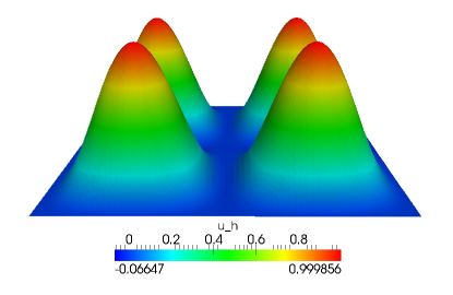
(a) finite element approximation to (5.1).

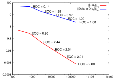
(b) $k=2$, piecewise quadratic FEs.

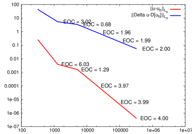
(c) $k=3$, piecewise cubic FEs.

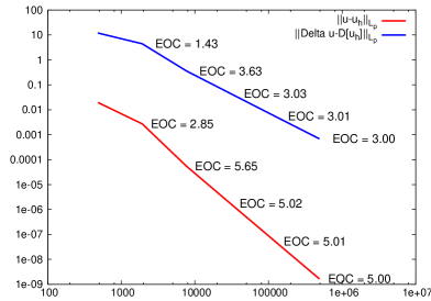
(d) $k=4$, piecewise quartic FEs.

Figure 2. Section 5.2 – The same test as in Figure 1 for the $2.1$–biharmonic problem, i.e., $p=2.1$ for $k=2\text{ and }3$.

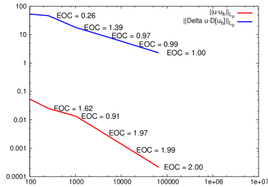
(a) $k=2$, piecewise quadratic FEs.

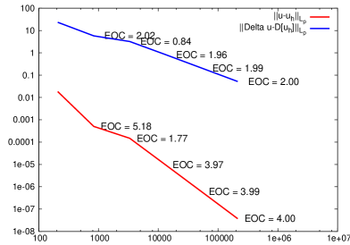
(b) $k=3$, piecewise cubic FEs.

Figure 3. Section 5.2 – The same test as in Figure 2 for the $10$–biharmonic problem,i.e., $p=10$.

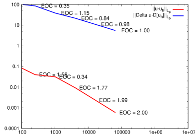
(a) $k=2$, piecewise quadratic FEs.

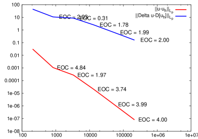
(b) $k=3$, piecewise cubic FEs.

5.3 Remark (computational observations).

Computationally, the convergence rates we observe are that

(5.2) $$\left\|u-u_{h}\right\|_{\operatorname{L}_{p}(\Omega)}=\begin{cases}\operatorname{O}(h^{2})\text{ when $k=2$}\\ \operatorname{O}(h^{k+1})\text{ otherwise }\end{cases}$$

and that

(5.3) $$\left\|\Delta u-\mathscr{D}[u_{h}]\right\|_{\operatorname{L}_{p}(\Omega)}=\operatorname{O}(h^{k-1}).$$

5.4 Remark (representation of $\boldsymbol{H}$).

Note that the dG Hessian $\boldsymbol{H}$ may be represented in a finite element space with different degree to $u_{h}\in\mathbb{V}$. Let $\mathbb{W}:=\mathbb{P}^{k-1}(\mathscr{T})$, the proof of Theorem 3.6 infers that we may choose to represent $\boldsymbol{H}[u_{h}]\in\mathbb{W}^{d\times d}$. For clarity of exposition we choose to use $\boldsymbol{H}[u_{h}]\in\mathbb{V}^{d\times d}$, however, we see no difficulty extending the arguments presented to the lower degree dG Hessian.

Numerically we observe the same convergence rates as in Remark 5.3 for the lower degree dG Hessian.

6. Conclusion and outlook

In this work we presented a dG finite element method for the $p$–biharmonic problem. To do this we introduced a auxiliary variable, the finite element Hessian and constructed a discrete variational problem.

We proved that the numerical solution of this discrete variational problem converges to the extrema of the continuous problem and that the finite element Hessian converges to the Hessian of the continuous extrema.

We foresee that this framework will prove useful when studying other (possibly more complicated) second order variational problems, such as discrete curvature problems like the affine maximal surface equation, which is the topic of ongoing research.