Communication-Efficient Algorithms for
Statistical Optimization

Abstract

We analyze two communication-efficient algorithms for distributed optimization in statistical settings involving large-scale data sets. The first algorithm is a standard averaging method that distributes the $N$ data samples evenly to $m$ machines, performs separate minimization on each subset, and then averages the estimates. We provide a sharp analysis of this average mixture algorithm, showing that under a reasonable set of conditions, the combined parameter achieves mean-squared error (MSE) that decays as $\mathcal{O}(N^{-1}+(N/m)^{-2})$. Whenever $m\leq\sqrt{N}$, this guarantee matches the best possible rate achievable by a centralized algorithm having access to all $N$ samples. The second algorithm is a novel method, based on an appropriate form of bootstrap subsampling. Requiring only a single round of communication, it has mean-squared error that decays as $\mathcal{O}(N^{-1}+(N/m)^{-3})$, and so is more robust to the amount of parallelization. In addition, we show that a stochastic gradient-based method attains mean-squared error decaying as $\mathcal{O}(N^{-1}+(N/m)^{-3/2})$, easing computation at the expense of a potentially slower MSE rate. We also provide an experimental evaluation of our methods, investigating their performance both on simulated data and on a large-scale regression problem from the internet search domain. In particular, we show that our methods can be used to efficiently solve an advertisement prediction problem from the Chinese SoSo Search Engine, which involves logistic regression with $N\approx 2.4\times 10^{8}$ samples and $d\approx 740,\!000$ covariates.

Keywords: Distributed Learning, Stochastic Optimization, Averaging, Subsampling

1 Introduction

Many procedures for statistical estimation are based on a form of (regularized) empirical risk minimization, meaning that a parameter of interest is estimated by minimizing an objective function defined by the average of a loss function over the data. Given the current explosion in the size and amount of data available in statistical studies, a central challenge is to design efficient algorithms for solving large-scale problem instances. In a centralized setting, there are many procedures for solving empirical risk minimization problems, among them standard convex programming approaches (e.g. Boyd and Vandenberghe, 2004) as well as stochastic approximation and optimization algorithms (Robbins and Monro, 1951; Hazan et al., 2006; Nemirovski et al., 2009). When the size of the dataset becomes extremely large, however, it may be infeasible to store all of the data on a single computer, or at least to keep the data in memory. Accordingly, the focus of this paper is the study of some distributed and communication-efficient procedures for empirical risk minimization.

Recent years have witnessed a flurry of research on distributed approaches to solving very large-scale statistical optimization problems. Although we cannot survey the literature adequately—the papers Nedić and Ozdaglar (2009); Ram et al. (2010); Johansson et al. (2009); Duchi et al. (2012a); Dekel et al. (2012); Agarwal and Duchi (2011); Recht et al. (2011); Duchi et al. (2012b) and references therein contain a sample of relevant work—we touch on a few important themes here. It can be difficult within a purely optimization-theoretic setting to show explicit benefits arising from distributed computation. In statistical settings, however, distributed computation can lead to gains in computational efficiency, as shown by a number of authors (Agarwal and Duchi, 2011; Dekel et al., 2012; Recht et al., 2011; Duchi et al., 2012b). Within the family of distributed algorithms, there can be significant differences in communication complexity: different computers must be synchronized, and when the dimensionality of the data is high, communication can be prohibitively expensive. It is thus interesting to study distributed estimation algorithms that require fairly limited synchronization and communication while still enjoying the greater statistical accuracy that is usually associated with a larger dataset.

With this context, perhaps the simplest algorithm for distributed statistical estimation is what we term the average mixture (Avgm) algorithm. It is an appealingly simple method: given $m$ different machines and a dataset of size $N$, first assign to each machine a (distinct) dataset of size $n=N/m$, then have each machine $i$ compute the empirical minimizer $\theta_{i}$ on its fraction of the data, and finally average all the parameter estimates $\theta_{i}$ across the machines. This approach has been studied for some classification and estimation problems by Mann et al. (2009) and McDonald et al. (2010), as well as for certain stochastic approximation methods by Zinkevich et al. (2010). Given an empirical risk minimization algorithm that works on one machine, the procedure is straightforward to implement and is extremely communication efficient, requiring only a single round of communication. It is also relatively robust to possible failures in a subset of machines and/or differences in speeds, since there is no repeated synchronization. When the local estimators are all unbiased, it is clear that the the Avgm procedure will yield an estimate that is essentially as good as that of an estimator based on all $N$ samples. However, many estimators used in practice are biased, and so it is natural to ask whether the method has any guarantees in a more general setting. To the best of our knowledge, however, no work has shown rigorously that the Avgm procedure generally has greater efficiency than the naive approach of using $n=N/m$ samples on a single machine.

This paper makes three main contributions. First, in Section 3, we provide a sharp analysis of the Avgm algorithm, showing that under a reasonable set of conditions on the population risk, it can indeed achieve substantially better rates than the naive approach. More concretely, we provide bounds on the mean-squared error (MSE) that decay as $\mathcal{O}((nm)^{-1}+n^{-2})$. Whenever the number of machines $m$ is less than the number of samples $n$ per machine, this guarantee matches the best possible rate achievable by a centralized algorithm having access to all $N=nm$ samples. In the special case of optimizing log likelihoods, the pre-factor in our bound involves the trace of the Fisher information, a quantity well-known to control the fundamental limits of statistical estimation. We also show how the result extends to stochastic programming approaches, exhibiting a stochastic gradient-descent based procedure that also attains convergence rates scaling as $\mathcal{O}((nm)^{-1})$, but with slightly worse dependence on different problem-specific parameters.

Our second contribution is to develop a novel extension of simple averaging. It is based on an appropriate form of resampling (Efron and Tibshirani, 1993; Hall, 1992; Politis et al., 1999), which we refer to as the subsampled average mixture (Savgm) approach. At a high level, the Savgm algorithm distributes samples evenly among $m$ processors or computers as before, but instead of simply returning the empirical minimizer, each processor further subsamples its own dataset in order to estimate the bias of its own estimate, and returns a subsample-corrected estimate. We establish that the Savgm algorithm has mean-squared error decaying as $\mathcal{O}(m^{-1}n^{-1}+n^{-3})$. As long as $m<n^{2}$, the subsampled method again matches the centralized gold standard in the first-order term, and has a second-order term smaller than the standard averaging approach.

Our third contribution is to perform a detailed empirical evaluation of both the Avgm and Savgm procedures, which we present in Sections 4 and 5. Using simulated data from normal and non-normal regression models, we explore the conditions under which the Savgm algorithm yields better performance than the Avgm algorithm; in addition, we study the performance of both methods relative to an oracle baseline that uses all $N$ samples. We also study the sensitivity of the algorithms to the number of splits $m$ of the data, and in the Savgm case, we investigate the sensitivity of the method to the amount of resampling. These simulations show that both Avgm and Savgm have favorable performance, even when compared to the unattainable “gold standard” procedure that has access to all $N$ samples. In Section 5, we complement our simulation experiments with a large logistic regression experiment that arises from the problem of predicting whether a user of a search engine will click on an advertisement. This experiment is large enough—involving $N\approx 2.4\times 10^{8}$ samples in $d\approx 740,000$ dimensions with a storage size of approximately 55 gigabytes—that it is difficult to solve efficiently on one machine. Consequently, a distributed approach is essential to take full advantage of this data set. Our experiments on this problem show that Savgm—with the resampling and correction it provides—gives substantial performance benefits over naive solutions as well as the averaging algorithm Avgm.

2 Background and problem set-up

We begin by setting up our decision-theoretic framework for empirical risk minimization, after which we describe our algorithms and the assumptions we require for our main theoretical results.

2.1 Empirical risk minimization

Let $\{f(\cdot;x),\;x\in\mathcal{X}\}$ be a collection of real-valued and convex loss functions, each defined on a set containing the convex set $\Theta\subseteq\mathbb{R}^{d}$. Let $P$ be a probability distribution over the sample space $\mathcal{X}$. Assuming that each function $x\mapsto f(\theta;\,x)$ is $P$-integrable, the population risk $F_{0}:\Theta\rightarrow\mathbb{R}$ is given by

$$F_{0}(\theta):=\mathbb{E}_{P}[f(\theta;X)]=\int_{\mathcal{X}}f(\theta;x)dP(x).$$ (1)

Our goal is to estimate the parameter vector minimizing the population risk, namely the quantity

$$\theta^{*}:=\mathop{\rm argmin}_{\theta\in\Theta}F_{0}(\theta)=\mathop{\rm argmin}_{\theta\in\Theta}\int_{\mathcal{X}}f(\theta;x)dP(x),$$ (2)

which we assume to be unique. In practice, the population distribution $P$ is unknown to us, but we have access to a collection $S$ of samples from the distribution $P$. Empirical risk minimization is based on estimating $\theta^{*}$ by solving the optimization problem

$$\widehat{\theta}\in\mathop{\rm argmin}_{\theta\in\Theta}\Big{\{}\frac{1}{|S|}\sum_{x\in S}f(\theta;x)\Big{\}}.$$ (3)

Throughout the paper, we impose some regularity conditions on the parameter space, the risk function $F_{0}$, and the instantaneous loss functions $f(\cdot;x):\Theta\rightarrow\mathbb{R}$. These conditions are standard in classical statistical analysis of $M$-estimators (e.g. Lehmann and Casella, 1998; Keener, 2010). Our first assumption deals with the relationship of the parameter space to the optimal parameter $\theta^{*}$.

Assumption A (Parameters)

The parameter space $\Theta\subset\mathbb{R}^{d}$ is a compact convex set, with $\theta^{*}\in\mathop{\rm int}\Theta$ and $\ell_{2}$-radius $R=\max\limits_{\theta\in\Theta}\left\|{\theta-\theta^{*}}\right\|_{2}$.

In addition, the risk function is required to have some amount of curvature. We formalize this notion in terms of the Hessian of $F_{0}$:

Assumption B (Local strong convexity)

The population risk is twice differentiable, and there exists a parameter $\lambda>0$ such that $\nabla^{2}F_{0}(\theta^{*})\succeq\lambda I_{d\times d}$.

Here $\nabla^{2}F_{0}(\theta)$ denotes the $d\times d$ Hessian matrix of the population objective $F_{0}$ evaluated at $\theta$, and we use $\succeq$ to denote the positive semidefinite ordering (i.e., $A\succeq B$ means that $A-B$ is positive semidefinite.) This local condition is milder than a global strong convexity condition and is required to hold only for the population risk $F_{0}$ evaluated at $\theta^{*}$. It is worth observing that some type of curvature of the risk is required for any method to consistently estimate the parameters $\theta^{*}$.

2.2 Averaging methods

Consider a data set consisting of $N=mn$ samples, drawn i.i.d. according to the distribution $P$. In the distributed setting, we divide this $N$-sample data set evenly and uniformly at random among a total of $m$ processors. (For simplicity, we have assumed the total number of samples is a multiple of $m$.) For $i=1,\ldots,m$, we let $S_{1,i}$ denote the data set assigned to processor $i$; by construction, it is a collection of $n$ samples drawn i.i.d. according to $P$, and the samples in subsets $S_{1,i}$ and $S_{1,j}$ are independent for $i\neq j$. In addition, for each processor $i$ we define the (local) empirical distribution $P_{1,i}$ and empirical objective $F_{1,i}$ via

$$P_{1,i}:=\frac{1}{|S_{1}|}\sum_{x\in S_{1,i}}\delta_{x},~{}~{}~{}\mbox{and}~{}~{}~{}F_{1,i}(\theta):=\frac{1}{|S_{1,i}|}\sum_{x\in S_{1,i}}f(\theta;x).$$ (4)

With this notation, the Avgm algorithm is very simple to describe:

Average mixture algorithm

1. For each $i\in\{1,\ldots,m\}$, processor $i$ uses its local dataset $S_{1,i}$ to compute the local empirical minimizer

   $$\theta_{1,i} \in\mathop{\rm argmin}_{\theta\in\Theta}\Big{\{}\underbrace{\frac{1}{|S_{1,i}|}\sum_{x\in S_{1,i}}f(\theta;x)}_{F_{1,i}(\theta)}\Big{\}}.$$ (5)

2. These $m$ local estimates are then averaged together—that is, we compute

   $$\overline{\theta}_{1}=\frac{1}{m}\sum_{i=1}^{m}\theta_{1,i}.$$ (6)

The subsampled average mixture (Savgm) algorithm is based on an additional level of sampling on top of the first, involving a fixed subsampling rate $\ratio\in[0,1]$. It consists of the following additional steps:

Subsampled average mixture algorithm

1. Each processor $i$ draws a subset $S_{2,i}$ of size $\left\lceil{rn}\right\rceil$ by sampling uniformly at random without replacement from its local data set $S_{1,i}$.

2. Each processor $i$ computes both the local empirical minimizers $\theta_{1,i}$ from equation (5) and the empirical minimizer

   $$\theta_{2,i} \in\mathop{\rm argmin}_{\theta\in\Theta}\Big{\{}\underbrace{\frac{1}{|S_{2,i}|}\sum_{x\in S_{2,i}}f(\theta;x)}_{F_{2,i}(\theta)}\Big{\}}.$$ (7)

3. In addition to the previous average (6), the Savgm algorithm computes the bootstrap average $\overline{\theta}_{2}:=\frac{1}{m}\sum_{i=1}^{m}\theta_{2,i}$, and then returns the weighted combination

   $$\overline{\theta}_{\textsc{Savgm}}:=\frac{\overline{\theta}_{1}-\ratio\overline{\theta}_{2}}{1-\ratio}.$$ (8)

The intuition for the weighted estimator (8) is similar to that for standard bias correction procedures using the bootstrap or subsampling (Efron and Tibshirani, 1993; Hall, 1992; Politis et al., 1999). Roughly speaking, if $b_{0}=\theta^{*}-\theta_{1}$ is the bias of the first estimator, then we may approximate $b_{0}$ by the subsampled estimate of bias $b_{1}=\theta^{*}-\theta_{2}$. Then, we use the fact that $b_{1}\approx b_{0}/\ratio$ to argue that $\theta^{*}\approx(\theta_{1}-\ratio\theta_{2})/(1-\ratio)$. The re-normalization enforces that the relative “weights” of $\overline{\theta}_{1}$ and $\overline{\theta}_{2}$ sum to 1.

The goal of this paper is to understand under what conditions—and in what sense—the estimators (6) and (8) approach the oracle performance, by which we mean the error of a centralized risk minimization procedure that is given access to all $N=nm$ samples.

Notation:

Before continuing, we define the remainder of our notation. We use $\ell_{2}$ to denote the usual Euclidean norm $\left\|{\theta}\right\|_{2}=(\sum_{j=1}^{d}\theta_{j}^{2})^{\frac{1}{2}}$. The $\ell_{2}$-operator norm of a matrix $A\in\mathbb{R}^{d_{1}\times d_{2}}$ is its maximum singular value, defined by

$$\left|\!\left|\!\left|{A}\right|\!\right|\!\right|_{2}:=\sup_{v\in\mathbb{R}^{d_{2}},\left\|{v}\right\|_{2}\leq 1}\|Av\|_{2}.$$

A convex function $F$ is $\lambda$-strongly convex on a set $U\subseteq\mathbb{R}^{d}$ if for arbitrary $u,v\in U$ we have

$$F(u)\geq F(v)+\left\langle\nabla F(v),u-v\right\rangle+\frac{\lambda}{2}\left\|{u-v}\right\|_{2}^{2}.$$

(If $F$ is not differentiable, we may replace $\nabla F$ with any subgradient of $F$.) We let $\otimes$ denote the Kronecker product, and for a pair of vectors $u,v$, we define the outer product $u\otimes v=uv^{\top}$. For a three-times differentiable function $F$, we denote the third derivative tensor by $\nabla^{3}F$, so that for each $u\in\mathop{\rm dom}F$ the operator $\nabla^{3}F(u):\mathbb{R}^{d\times d}\rightarrow\mathbb{R}^{d}$ is linear and satisfies the relation

$$\left[\nabla^{3}F(u)(v\otimes v)\right]_{i}=\sum_{j,k=1}^{d}\left(\frac{\partial^{3}}{\partial u_{i}\partial u_{j}\partial u_{k}}F(u)\right)v_{j}v_{k}.$$

We denote the indicator function of an event $\mathcal{E}$ by $1_{\left({\mathcal{E}}\right)}$, which is 1 if $\mathcal{E}$ is true and 0 otherwise.

3 Theoretical results

Having described the Avgm and Savgm algorithms, we now turn to statements of our main theorems on their statistical properties, along with some consequences and comparison to past work.

3.1 Smoothness conditions

In addition to our previously stated assumptions on the population risk, we require regularity conditions on the empirical risk functions. It is simplest to state these in terms of the functions $\theta\mapsto f(\theta;x)$, and we note that, as with Assumption B, we require these to hold only locally around the optimal point $\theta^{*}$, in particular within some Euclidean ball $U=\{\theta\in\mathbb{R}^{d}\mid\left\|{\theta^{*}-\theta}\right\|_{2}\leq\rho\}\subseteq\Theta$ of radius $\rho>0$.

Assumption C (Smoothness)

There are finite constants $G,H$ such that the first and the second partial derivatives of $f$ exist and satisfy the bounds

$$\mathbb{E}[\left\|{\nabla f(\theta;X)}\right\|_{2}^{8}]\leq G^{8}~{}~{}~{}\mbox{and}~{}~{}~{}\mathbb{E}[\left|\!\left|\!\left|{\nabla^{2}f(\theta;X)-\nabla^{2}F_{0}(\theta)}\right|\!\right|\!\right|_{2}^{8}]\leq H^{8}\quad\mbox{for all $\theta\in U$.}$$

In addition, for any $x\in\mathcal{X}$, the Hessian matrix $\nabla^{2}f(\theta;x)$ is $L(x)$-Lipschitz continuous, meaning that

$$\left|\!\left|\!\left|{\nabla^{2}f(\theta^{\prime};x)-\nabla^{2}f(\theta;x)}\right|\!\right|\!\right|_{2}\leq L(x)\left\|{\theta^{\prime}-\theta}\right\|_{2}\quad\mbox{ for all $\theta,\theta^{\prime}\in U$.}$$ (9)

We require that $\mathbb{E}[L(X)^{8}]\leq L^{8}$ and $\mathbb{E}[(L(X)-\mathbb{E}[L(X)])^{8}]\leq L^{8}$ for some finite constant $L$.

It is an important insight of our analysis that some type of smoothness condition on the Hessian matrix, as in the Lipschitz condition (9), is essential in order for simple averaging methods to work. This necessity is illustrated by the following example:

Example 1 (Necessity of Hessian conditions)

Let $X$ be a Bernoulli variable with parameter $\frac{1}{2}$, and consider the loss function

$$f(\theta;x)=\begin{cases}\theta^{2}-\theta&\mbox{if}~{}x=0\\ \theta^{2}1_{\left({\theta\leq 0}\right)}+\theta&\mbox{if~{}}x=1,\end{cases}$$ (10)

where $1_{\left({\theta\leq 0}\right)}$ is the indicator of the event $\{\theta\leq 0\}$. The associated population risk is $F_{0}(\theta)=\frac{1}{2}(\theta^{2}+\theta^{2}1_{\left({\theta\leq 0}\right)})$. Since $|F_{0}^{\prime}(w)-F_{0}^{\prime}(v)|\leq 2|w-v|$, the population risk is strongly convex and smooth, but it has discontinuous second derivative. The unique minimizer of the population risk is $\theta^{*}=0$, and by an asymptotic expansion given in Appendix A, it can be shown that $\mathbb{E}[\theta_{1,i}]=\Omega(n^{-\frac{1}{2}})$. Consequently, the bias of $\overline{\theta}_{1}$ is $\Omega(n^{-\frac{1}{2}})$, and the Avgm algorithm using $N=mn$ observations must suffer mean squared error $\mathbb{E}[(\overline{\theta}_{1}-\theta^{*})^{2}]=\Omega(n^{-1})$.

The previous example establishes the necessity of a smoothness condition. However, in a certain sense, it is a pathological case: both the smoothness condition given in Assumption C and the local strong convexity condition given in Assumption B are relatively innocuous for practical problems. For instance, both conditions will hold for standard forms of regression, such as linear and logistic, as long as the population data covariance matrix is not rank deficient and the data has suitable moments. Moreover, in the linear regression case, one has $L=0$.

3.2 Bounds for simple averaging

We now turn to our first theorem that provides guarantees on the statistical error associated with the Avgm procedure. We recall that $\theta^{*}$ denotes the minimizer of the population objective function $F_{0}$, and that for each $i\in\{1,\ldots,m\}$, we use $S_{i}$ to denote a dataset of $n$ independent samples. For each $i$, we use $\theta_{i}\in\mathop{\rm argmin}_{\theta\in\Theta}\{\frac{1}{n}\sum_{x\in S_{i}}f(\theta;x)\}$ to denote a minimizer of the empirical risk for the dataset $S_{i}$, and we define the averaged vector $\overline{\theta}=\frac{1}{m}\sum_{i=1}^{m}\theta_{i}$. The following result bounds the mean-squared error between this averaged estimate and the minimizer $\theta^{*}$ of the population risk.

Theorem 1

Under Assumptions A through C, the mean-squared error is upper bounded as

$$\mathbb{E}\left[\left\|{\overline{\theta}-\theta^{*}}\right\|_{2}^{2}\right]\leq\frac{2}{nm}\mathbb{E}\left[\left\|{\nabla^{2}F_{0}(\theta^{*})^{-1}\nabla f(\theta^{*};X)}\right\|_{2}^{2}\right]$$ (11)

$$\qquad\qquad~{}+\frac{c}{\lambda^{2}n^{2}}\left(H^{2}\log d+\frac{L^{2}G^{2}}{\lambda^{2}}\right)\mathbb{E}\left[\left\|{\nabla^{2}F_{0}(\theta^{*})^{-1}\nabla f(\theta^{*};X)}\right\|_{2}^{2}\right]$$

$$\qquad\qquad~{}+\mathcal{O}(m^{-1}n^{-2})+\mathcal{O}(n^{-3}),$$

where $c$ is a numerical constant.

A slightly weaker corollary of Theorem 1 makes it easier to parse. In particular, note that

$$\left\|{\nabla^{2}F_{0}(\theta^{*})^{-1}\nabla f(\theta^{*};x)}\right\|_{2}\;\stackrel{{\scriptstyle(i)}}{{\leq}}\;\left|\!\left|\!\left|{\nabla^{2}F_{0}(\theta^{*})^{-1}}\right|\!\right|\!\right|_{2}\left\|{\nabla f(\theta^{*};x)}\right\|_{2}\;\stackrel{{\scriptstyle(ii)}}{{\leq}}\;\frac{1}{\lambda}\left\|{\nabla f(\theta^{*};x)}\right\|_{2},$$ (12)

where step (i) follows from the inequality $\left|\!\left|\!\left|{Ax}\right|\!\right|\!\right|_{2}\leq\left|\!\left|\!\left|{A}\right|\!\right|\!\right|\left\|{x}\right\|_{2}$, valid for any matrix $A$ and vector $x$; and step (ii) follows from Assumption B. In addition, Assumption C implies $\mathbb{E}[\left\|{\nabla f(\theta^{*};X)}\right\|_{2}^{2}]\leq G^{2}$, and putting together the pieces, we have established the following.

Corollary 2

Under the same conditions as Theorem 1,

$$\mathbb{E}\left[\left\|{\overline{\theta}-\theta^{*}}\right\|_{2}^{2}\right] \leq\frac{2G^{2}}{\lambda^{2}nm}+\frac{cG^{2}}{\lambda^{4}n^{2}}\left(H^{2}\log d+\frac{L^{2}G^{2}}{\lambda^{2}}\right)+\mathcal{O}(m^{-1}n^{-2})+\mathcal{O}(n^{-3}).$$ (13)

This upper bound shows that the leading term decays proportionally to $(nm)^{-1}$, with the pre-factor depending inversely on the strong convexity constant $\lambda$ and growing proportionally with the bound $G$ on the loss gradient. Although easily interpretable, the upper bound (13) can be loose, since it is based on the relatively weak series of bounds (12).

The leading term in our original upper bound (11) involves the product of the gradient $\nabla f(\theta^{*};X)$ with the inverse Hessian. In many statistical settings, including the problem of linear regression, the effect of this matrix-vector multiplication is to perform some type of standardization. When the loss $f(\cdot;x):\Theta\rightarrow\mathbb{R}$ is actually the negative log-likelihood $\ell(x\mid\theta)$ for a parametric family of models $\{P_{\theta}\}$, we can make this intuition precise. In particular, under suitable regularity conditions (e.g. Lehmann and Casella, 1998, Chapter 6), we can define the Fisher information matrix

$$I(\theta^{*}):=\mathbb{E}\left[\nabla\ell(X\mid\theta^{*})\nabla\ell(X\mid\theta^{*})^{\top}\right]=\mathbb{E}[\nabla^{2}\ell(X\mid\theta^{*})].$$

Recalling that $N=mn$ is the total number of samples available, let us define the neighborhood $B_{2}(\theta,t):=\{\theta^{\prime}\in\mathbb{R}^{d}:\left\|{\theta^{\prime}-\theta}\right\|_{2}\leq t\}$. Then under our assumptions, the Hájek-Le Cam minimax theorem (van der Vaart, 1998, Theorem 8.11) guarantees for any estimator $\widehat{\theta}_{N}$ based on $N$ samples that

$$\lim_{c\rightarrow\infty}\liminf_{N\rightarrow\infty}\sup_{\theta\in B_{2}(\theta^{*},c/\sqrt{N})}N\,\mathbb{E}_{\theta}\left[\big{\|}{\widehat{\theta}_{N}-\theta}\big{\|}_{2}^{2}\right]\geq\mathop{\rm tr}(I(\theta^{*})^{-1}).$$

In connection with Theorem 1, we obtain:

Corollary 3

In addition to the conditions of Theorem 1, suppose that the loss functions $f(\cdot;x)$ are the negative log-likelihood $\ell(x\mid\theta)$ for a parametric family $\{P_{\theta},\>\theta\in\Theta\}$. Then the mean-squared error is upper bounded as

$$\mathbb{E}\left[\left\|{\overline{\theta}_{1}-\theta^{*}}\right\|_{2}^{2}\right]\leq\frac{2}{N}\mathop{\rm tr}(I(\theta^{*})^{-1})+\frac{cm^{2}\mathop{\rm tr}(I(\theta^{*})^{-1})}{\lambda^{2}N^{2}}\left(H^{2}\log d+\frac{L^{2}G^{2}}{\lambda^{2}}\right)+\mathcal{O}(mN^{-2}),$$

where $c$ is a numerical constant.

Proof: Rewriting the log-likelihood in the notation of Theorem 1, we have $\nabla\ell(x\mid\theta^{*})=\nabla f(\theta^{*};x)$ and all we need to note is that

$$I(\theta^{*})^{-1} =\mathbb{E}\left[I(\theta^{*})^{-1}\nabla\ell(X\mid\theta^{*})\nabla\ell(X\mid\theta^{*})^{\top}I(\theta^{*})^{-1}\right]$$

$$=\mathbb{E}\Big{[}\left(\nabla^{2}F_{0}(\theta^{*})^{-1}\nabla f(\theta^{*};X)\right)\left(\nabla^{2}F_{0}(\theta^{*})^{-1}\nabla f(\theta^{*};X)\right)^{\top}\Big{]}.$$

Now apply the linearity of the trace and use the fact that $\mathop{\rm tr}(uu^{\top})=\left\|{u}\right\|_{2}^{2}$.  

Except for the factor of two in the bound, Corollary 3 shows that Theorem 1 essentially achieves the best possible result. The important aspect of our bound, however, is that we obtain this convergence rate without calculating an estimate on all $N=mn$ samples: instead, we calculate $m$ independent estimators, and then average them to attain the convergence guarantee. We remark that an inspection of our proof shows that, at the expense of worse constants on higher order terms, we can reduce the factor of $2/mn$ on the leading term in Theorem 1 to $(1+c)/mn$ for any constant $c>0$; as made clear by Corollary 3, this is unimprovable, even by constant factors.

As noted in the introduction, our bounds are certainly to be expected for unbiased estimators, since in such cases averaging $m$ independent solutions reduces the variance by $1/m$. In this sense, our results are similar to classical distributional convergence results in $M$-estimation: for smooth enough problems, $M$-estimators behave asymptotically like averages (van der Vaart, 1998; Lehmann and Casella, 1998), and averaging multiple independent realizations reduces their variance. However, it is often desirable to use biased estimators, and such bias introduces difficulty in the analysis, which we explore more in the next section. We also note that in contrast to classical asymptotic results, our results are applicable to finite samples and give explicit upper bounds on the mean-squared error. Lastly, our results are not tied to a specific model, which allows for fairly general sampling distributions.

3.3 Bounds for subsampled mixture averaging

When the number of machines $m$ is relatively small, Theorem 1 and Corollary 2 show that the convergence rate of the Avgm algorithm is mainly determined by the first term in the bound (11), which is at most $\frac{G^{2}}{\lambda^{2}mn}$. In contrast, when the number of processors $m$ grows, the second term in the bound (11), in spite of being $\mathcal{O}(n^{-2})$, may have non-negligible effect. This issue is exacerbated when the local strong convexity parameter $\lambda$ of the risk $F_{0}$ is close to zero or the Lipschitz continuity constant $H$ of $\nabla f$ is large. This concern motivated our development of the subsampled average mixture (Savgm) algorithm, to which we now return.

Due to the additional randomness introduced by the subsampling in Savgm, its analysis requires an additional smoothness condition. In particular, recalling the Euclidean $\rho$-neighborhood $U$ of the optimum $\theta^{*}$, we require that the loss function $f$ is (locally) smooth through its third derivatives.

Assumption D (Strong smoothness)

For each $x\in\mathcal{X}$, the third derivatives of $f$ are $M(x)$-Lipschitz continuous, meaning that

$$\left\|{\left(\nabla^{3}f(\theta;x)-\nabla^{3}f(\theta^{\prime};x)\right)(u\otimes u)}\right\|_{2}\leq M(x)\left\|{\theta-\theta^{\prime}}\right\|_{2}\left\|{u}\right\|_{2}^{2}\quad\mbox{for all $\theta,\theta^{\prime}\in U$, and $u\in\mathbb{R}^{d}$,}$$

where $\mathbb{E}[M^{8}(X)]\leq M^{8}$ for some constant $M<\infty$.

It is easy to verify that Assumption D holds for least-squares regression with $M=0$. It also holds for various types of non-linear regression problems (e.g., logistic, multinomial etc.) as long as the covariates have finite eighth moments.

With this set-up, our second theorem establishes that bootstrap sampling yields improved performance:

Theorem 4

Under Assumptions A through D, the output $\overline{\theta}_{\textsc{Savgm}}=(\overline{\theta}_{1}-\ratio\overline{\theta}_{2})/(1-\ratio)$ of the bootstrap Savgm algorithm has mean-squared error bounded as

$$\mathbb{E}\left[\left\|{\overline{\theta}_{\textsc{Savgm}}-\theta^{*}}\right\|_{2}^{2}\right] \leq\frac{2+3\ratio}{(1-\ratio)^{2}}\cdot\frac{1}{nm}\mathbb{E}\left[\left\|{\nabla^{2}F_{0}(\theta^{*})^{-1}\nabla f(\theta^{*};X)}\right\|_{2}^{2}\right]$$ (14)

$$+c\left(\frac{M^{2}G^{6}}{\lambda^{6}}+\frac{G^{4}L^{2}d\log d}{\lambda^{4}}\right)\left(\frac{1}{\ratio(1-\ratio)^{2}}\right)n^{-3}+\mathcal{O}\left(\frac{1}{(1-\ratio)^{2}}m^{-1}n^{-2}\right)$$

for a numerical constant $c$.

Comparing the conclusions of Theorem 4 to those of Theorem 1, we see that the the $\mathcal{O}(n^{-2})$ term in the bound (11) has been eliminated. The reason for this elimination is that subsampling at a rate reduces the bias of the Savgm algorithm to $\mathcal{O}(n^{-3})$, whereas in contrast, the bias of the Avgm algorithm induces terms of order $n^{-2}$. Theorem 4 suggests that the performance of the Savgm algorithm is affected by the subsampling rate ; in order to minimize the upper bound (14) in the regime $m<N^{2/3}$, the optimal choice is of the form $\ratio\propto C\sqrt{m}/n=Cm^{3/2}/N$ where $C\approx(G^{2}/\lambda^{2})\max\{MG/\lambda,L\sqrt{d\log d}\}$. Roughly, as the number of machines $m$ becomes larger, we may increase , since we enjoy averaging affects from the Savgm algorithm.

Let us consider the relative effects of having larger numbers of machines $m$ for both the Avgm and Savgm algorithms, which provides some guidance to selecting $m$ in practice. We define $\sigma^{2}=\mathbb{E}[\left\|{\nabla^{2}F_{0}(\theta^{*})^{-1}\nabla f(\theta^{*};X)}\right\|_{2}^{2}]$ to be the asymptotic variance. Then to obtain the optimal convergence rate of $\sigma^{2}/N$, we must have

$$\frac{1}{\lambda^{2}}\max\left\{H^{2}\log d,L^{2}G^{2}\right\}\frac{m^{2}}{N^{2}}\sigma^{2}\leq\frac{\sigma^{2}}{N}~{}~{}~{}\mbox{or}~{}~{}~{}m\leq N^{\frac{1}{2}}\sqrt{\frac{\lambda^{2}}{\max\{H^{2}\log d,L^{2}G^{2}/\lambda^{2}\}}}$$ (15)

in Theorem 1. Applying the bound of Theorem 4, we find that to obtain the same rate we require

$$\max\left\{\frac{M^{2}G^{2}}{\lambda^{6}},\frac{L^{2}d\log d}{\lambda^{4}}\right\}\frac{G^{4}m^{3}}{\ratio N^{3}}\leq\frac{(1+\ratio)\sigma^{2}}{N}~{}\mbox{or}~{}m\leq N^{\frac{2}{3}}\left(\frac{\lambda^{4}\ratio(1+\ratio)\sigma^{2}}{\max\left\{M^{2}G^{6}/\lambda^{2},G^{4}L^{2}d\log d\right\}}\right)^{\frac{1}{3}}\!\!\!.$$

Now suppose that we replace with $Cm^{3/2}/N$ as in the previous paragraph. Under the conditions $\sigma^{2}\approx G^{2}$ and $\ratio=o(1)$, we then find that

$$m\leq N^{\frac{2}{3}}\left(\frac{\lambda^{2}\sigma^{2}m^{3/2}}{G^{2}\max\left\{MG/\lambda,L\sqrt{d\log d}\right\}N}\right)^{\frac{1}{3}}~{}\mbox{or}~{}m\leq N^{\frac{2}{3}}\left(\frac{\lambda^{2}}{\max\left\{MG/\lambda,L\sqrt{d\log d}\right\}}\right)^{\frac{2}{3}}.$$ (16)

Comparing inequalities (15) and (16), we see that in both cases $m$ may grow polynomially with the global sample size $N$ while still guaranteeing optimal convergence rates. On one hand, this asymptotic growth is faster in the subsampled case (16); on the other hand, the dependence on the dimension $d$ of the problem is more stringent than the standard averaging case (15). As the local strong convexity constant $\lambda$ of the population risk shrinks, both methods allow less splitting of the data, meaning that the sample size per machine must be larger. This limitation is intuitive, since lower curvature for the population risk means that the local empirical risks associated with each machine will inherit lower curvature as well, and this effect will be exacerbated with a small local sample size per machine. Averaging methods are, of course, not a panacea: the allowed number of partitions $m$ does not grow linearly in either case, so blindly increasing the number of machines proportionally to the total sample size $N$ will not lead to a useful estimate.

In practice, an optimal choice of may not be apparent, which may necessitate cross validation or another type of model evaluation. We leave as intriguing open questions whether computing multiple subsamples at each machine can yield improved performance or reduce the variance of the Savgm procedure, and whether using estimates based on resampling the data with replacement, as opposed to without replacement as considered here, can yield improved performance.

3.4 Time complexity

In practice, the exact empirical minimizers assumed in Theorems 1 and 4 may be unavailable. Instead, we need to use a finite number of iterations of some optimization algorithm in order to obtain reasonable approximations to the exact minimizers. In this section, we sketch an argument that shows that both the Avgm algorithm and the Savgm algorithm can use such approximate empirical minimizers, and as long as the optimization error is sufficiently small, the resulting averaged estimate achieves the same order-optimal statistical error. Here we provide the arguments only for the Avgm algorithm; the arguments for the Savgm algorithm are analogous.

More precisely, suppose that each processor runs a finite number of iterations of some optimization algorithm, thereby obtaining the vector $\theta_{i}^{\prime}$ as an approximate minimizer of the objective function $F_{1,i}$. Thus, the vector $\theta_{i}^{\prime}$ can be viewed as an approximate form of $\theta_{i}$, and we let $\overline{\theta}^{\prime}=\frac{1}{m}\sum_{i=1}^{m}\theta_{i}^{\prime}$ denote the average of these approximate minimizers, which corresponds to the output of the approximate Avgm algorithm. With this notation, we have

$$\mathbb{E}\left[\big{\|}{\overline{\theta}^{\prime}-\theta^{*}}\big{\|}_{2}^{2}\right]\;\stackrel{{\scriptstyle(i)}}{{\leq}}\;2\mathbb{E}[\left\|{\overline{\theta}-\theta^{*}}\right\|_{2}^{2}]+2\mathbb{E}\left[\big{\|}{\overline{\theta}^{\prime}-\overline{\theta}}\big{\|}_{2}^{2}\right]\;\stackrel{{\scriptstyle(ii)}}{{\leq}}\;2\mathbb{E}[\left\|{\overline{\theta}-\theta^{*}}\right\|_{2}^{2}]+2\mathbb{E}[\left\|{\theta_{1}^{\prime}-\theta_{1}}\right\|_{2}^{2}],$$ (17)

where step (i) follows by triangle inequality and the elementary bound $(a+b)^{2}\leq 2a^{2}+2b^{2}$; step (ii) follows by Jensen’s inequality. Consequently, suppose that processor $i$ runs enough iterations to obtain an approximate minimizer $\theta^{\prime}_{1}$ such that

$$\mathbb{E}[\left\|{\theta_{i}^{\prime}-\theta_{i}}\right\|_{2}^{2}] =\mathcal{O}((mn)^{-2}).$$ (18)

When this condition holds, the bound (17) shows that the average $\overline{\theta}^{\prime}$ of the approximate minimizers shares the same convergence rates provided by Theorem 1.

But how long does it take to compute an approximate minimizer $\theta^{\prime}_{i}$ satisfying condition (18)? Assuming processing one sample requires one unit of time, we claim that this computation can be performed in time $\mathcal{O}(n\log(mn))$. In particular, the following two-stage strategy, involving a combination of stochastic gradient descent (see the following subsection for more details) and standard gradient descent, has this complexity:

1. As shown in the proof of Theorem 1, with high probability, the empirical risk $F_{1}$ is strongly convex in a ball $B_{\rho}(\theta_{1})$ of constant radius $\rho>0$ around $\theta_{1}$. Consequently, performing stochastic gradient descent on $F_{1}$ for $\mathcal{O}(\log^{2}(mn)/\rho^{2})$ iterations yields an approximate minimizer that falls within $B_{\rho}(\theta_{1})$ with high probability (e.g. Nemirovski et al., 2009, Proposition 2.1). Note that the radius $\rho$ for local strong convexity is a property of the population risk $F_{0}$ we use as a prior knowledge.

2. This initial estimate can be further improved by a few iterations of standard gradient descent. Under local strong convexity of the objective function, gradient descent is known to converge at a geometric rate (see, e.g. Nocedal and Wright, 2006; Boyd and Vandenberghe, 2004), so $\mathcal{O}(\log(1/\epsilon))$ iterations will reduce the error to order $\epsilon$. In our case, we have $\epsilon=(mn)^{-2}$, and since each iteration of standard gradient descent requires $\mathcal{O}(n)$ units of time, a total of $\mathcal{O}(n\log(mn))$ time units are sufficient to obtain a final estimate $\theta_{1}^{\prime}$ satisfying condition (18).

Overall, we conclude that the speed-up of the Avgm  relative to the naive approach of processing all $N=mn$ samples on one processor, is at least of order $m/\log(N)$.

3.5 Stochastic gradient descent with averaging

The previous strategy involved a combination of stochastic gradient descent and standard gradient descent. In many settings, it may be appealing to use only a stochastic gradient algorithm, due to their ease of their implementation and limited computational requirements. In this section, we describe an extension of Theorem 1 to the case in which each machine computes an approximate minimizer using only stochastic gradient descent.

Stochastic gradient algorithms have a lengthy history in statistics, optimization, and machine learning (Robbins and Monro, 1951; Polyak and Juditsky, 1992; Nemirovski et al., 2009; Rakhlin et al., 2012). Let us begin by briefly reviewing the basic form of stochastic gradient descent (SGD). Stochastic gradient descent algorithms iteratively update a parameter vector $\theta^{t}$ over time based on randomly sampled gradient information. Specifically, at iteration $t$, a sample $X_{t}$ is drawn at random from the distribution $P$ (or, in the case of a finite set of data $\{X_{1},\ldots,X_{n}\}$, a sample $X_{t}$ is chosen from the data set). The method then performs the following two steps:

$$\theta^{t+\frac{1}{2}}=\theta^{t}-\eta_{t}\nabla f(\theta^{t};X_{t})~{}~{}~{}\mbox{and}~{}~{}~{}\theta^{t+1}=\mathop{\rm argmin}_{\theta\in\Theta}\left\{\big{\|}{\theta-\theta^{t+\frac{1}{2}}}\big{\|}_{2}^{2}\right\}.$$ (19)

Here $\eta_{t}>0$ is a stepsize, and the first update in (19) is a gradient descent step with respect to the random gradient $\nabla f(\theta^{t};X_{t})$. The method then projects the intermediate point $\theta^{t+\frac{1}{2}}$ back onto the constraint set $\Theta$ (if there is a constraint set). The convergence of SGD methods of the form (19) has been well-studied, and we refer the reader to the papers by Polyak and Juditsky (1992), Nemirovski et al. (2009), and Rakhlin et al. (2012) for deeper investigations.

To prove convergence of our stochastic gradient-based averaging algorithms, we require the following smoothness and strong convexity condition, which is an alternative to the Assumptions B and C used previously.

Assumption E (Smoothness and Strong Convexity II)

There exists a function $L:\mathcal{X}\rightarrow\mathbb{R}_{+}$ such that

$$\left|\!\left|\!\left|{\nabla^{2}f(\theta;x)-\nabla^{2}f(\theta^{*};x)}\right|\!\right|\!\right|_{2}\leq L(x)\left\|{\theta-\theta^{*}}\right\|_{2}~{}~{}~{}\mbox{for~{}all}~{}x\in\mathcal{X},$$

and $\mathbb{E}[L^{2}(X)]\leq L^{2}<\infty$. There are finite constants $G$ and $H$ such that

$$\mathbb{E}[\left\|{\nabla f(\theta;X)}\right\|_{2}^{4}]\leq G^{4},\quad\mbox{and}\quad\mathbb{E}[\left|\!\left|\!\left|{\nabla^{2}f(\theta^{*};X)}\right|\!\right|\!\right|_{2}^{4}]\leq H^{4}\quad\mbox{for each fixed}~{}\theta\in\Theta.$$

In addition, the population function $F_{0}$ is $\lambda$-strongly convex over the space $\Theta$, meaning that

$$\nabla^{2}F_{0}(\theta)\succeq\lambda I_{d\times d}\quad\mbox{for all}~{}\theta\in\Theta.$$ (20)

Assumption E does not require as many moments as does Assumption C, but it does require each moment bound to hold globally, that is, over the entire space $\Theta$, rather than only in a neighborhood of the optimal point $\theta^{*}$. Similarly, the necessary curvature—in the form of the lower bound on the Hessian matrix $\nabla^{2}F_{0}$—is also required to hold globally, rather than only locally. Nonetheless, Assumption E holds for many common problems; for instance, it holds for any linear regression problem in which the covariates have finite fourth moments and the domain $\Theta$ is compact.

The averaged stochastic gradient algorithm (SGDavgm) is based on the following two steps:

1. Given some constant $c>1$, each machine performs $n$ iterations of stochastic gradient descent (19) on its local dataset of $n$ samples using the stepsize $\eta_{t}=\frac{c}{\lambda t}$, then outputs the resulting local parameter $\theta^{\prime}_{i}$.

2. The algorithm computes the average $\overline{\theta}^{n}=\frac{1}{m}\sum_{i=1}^{m}\theta^{\prime}_{i}$.

The following result characterizes the mean-squared error of this procedure in terms of the constants

$$\alpha:=4c^{2}\quad\mbox{and}\quad\beta:=\max\left\{\left\lceil{\frac{cH}{\lambda}}\right\rceil,\frac{c\alpha^{3/4}G^{3/2}}{(c-1)\lambda^{5/2}}\left(\frac{\alpha^{1/4}LG^{1/2}}{\lambda^{1/2}}+\frac{4G+HR}{\rho^{3/2}}\right)\right\}.$$

Theorem 5

Under Assumptions A and E, the output $\overline{\theta}^{n}$ of the Savgm algorithm has mean-squared error upper bounded as

$$\mathbb{E}\left[\big{\|}{\overline{\theta}^{n}-\theta^{*}}\big{\|}_{2}^{2}\right]\leq\frac{\alpha G^{2}}{\lambda^{2}mn}+\frac{\beta^{2}}{n^{3/2}}.$$ (21)

Theorem 5 shows that the averaged stochastic gradient descent procedure attains the optimal convergence rate $\mathcal{O}(N^{-1})$ as a function of the total number of observations $N=mn$. The constant and problem-dependent factors are somewhat worse than those in the earlier results we presented in Theorems 1 and 4, but the practical implementability of such a procedure may in some circumstances outweigh those differences. We also note that the second term of order $\mathcal{O}(n^{-3/2})$ may be reduced to $\mathcal{O}(n^{(2-2k)/k})$ for any $k\geq 4$ by assuming the existence of $k$th moments in Assumption E; we show this in passing after our proof of the theorem in Appendix D. It is not clear whether a bootstrap correction is possible for the stochastic-gradient based estimator; such a correction could be significant, because the term $\beta^{2}/n^{3/2}$ arising from the bias in the stochastic gradient estimator may be non-trivial. We leave this question to future work.

4 Performance on synthetic data

In this section, we report the results of simulation studies comparing the Avgm, Savgm, and SGDavgm methods, as well as a trivial method using only a fraction of the data available on a single machine. For each of our simulated experiments, we use a fixed total number of samples $N=100,\!000$, but we vary the number of parallel splits $m$ of the data (and consequently, the local dataset sizes $n=N/m$) and the dimensionality $d$ of the problem solved.

For our experiments, we simulate data from one of three regression models:

$$y =\left\langle u,x\right\rangle+\varepsilon,$$ (22a)

$$y =\left\langle u,x\right\rangle+\sum_{j=1}^{d}v_{j}x_{j}^{3}+\varepsilon,~{}~{}~{}~{}\mbox{or}~{}$$ (22b)

$$y =\left\langle u,x\right\rangle+h(x)|\varepsilon|,$$ (22c)

where $\varepsilon\sim N(0,1)$, and $h$ is a function to be specified. Specifically, the data generation procedure is as follows. For each individual simulation, we choose fixed vector $u\in\mathbb{R}^{d}$ with entries $u_{i}$ distributed uniformly in $[0,1]$ (and similarly for $v$), and we set $h(x)=\sum_{j=1}^{d}(x_{j}/2)^{3}$. The models (22a) through (22c) provide points on a curve from correctly-specified to grossly mis-specified models, so models (22b) and (22c) help us understand the effects of subsampling in the Savgm algorithm. (In contrast, the standard least-squares estimator is unbiased for model (22a).) The noise variable $\varepsilon$ is always chosen as a standard Gaussian variate $N(0,1)$, independent from sample to sample.

In our simulation experiments we use the least-squares loss

$$f(\theta;(x,y)):=\frac{1}{2}(\left\langle\theta,x\right\rangle-y)^{2}.$$

The goal in each experiment is to estimate the vector $\theta^{*}$ minimizing $F_{0}(\theta):=\mathbb{E}[f(\theta;(X,Y))]$. For each simulation, we generate $N$ samples according to either the model (22a) or (22c). For each $m\in\{2,4,8,16,32,64,128\}$, we estimate $\theta^{*}=\arg\min_{\theta}F_{0}(\theta)$ using a parallel method with data split into $m$ independent sets of size $n=N/m$, specifically

1. The Avgm method

2. The Savgm method with several settings of the subsampling ratio

3. The SGDavgm method with stepsize $\eta_{t}=d/(10(d+t))$, which gave good performance.

In addition to (i)–(iii), we also estimate $\theta^{*}$ with

1. The empirical minimizer of a single split of the data of size $n=N/m$

2. The empirical minimizer on the full dataset (the oracle solution).

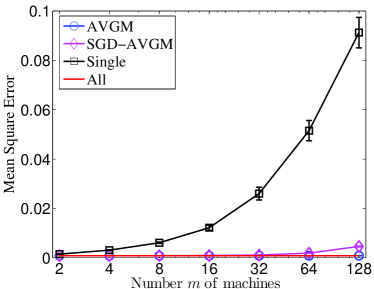
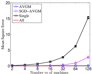
(a) $d=20$	(b) $d=200$

Figure 1: The error $\|{\widehat{\theta}-\theta^{*}}\|_{2}^{2}$ versus number of machines, with standard errors across twenty simulations, for solving least squares with data generated according to the normal model (22a). The oracle least-squares estimate using all $N$ samples is given by the line “All,” while the line “Single” gives the performance of the naive estimator using only $n=N/m$ samples.

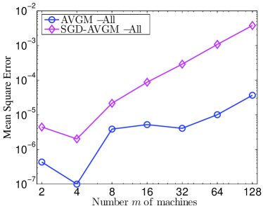
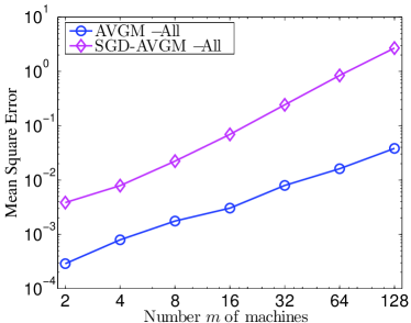
(a) $d=20$	(b) $d=200$

Figure 2: Comparison of Avgm and SGDavgm methods as in Figure 1 plotted on logarithmic scale. The plot shows $\|{\widehat{\theta}-\theta^{*}}\|_{2}^{2}-\left\|{\theta_{N}-\theta^{*}}\right\|_{2}^{2}$, where $\theta_{N}$ is the oracle least-squares estimator using all $N$ data samples.

4.1 Averaging methods

For our first set of experiments, we study the performance of the averaging methods (Avgm and Savgm), showing their scaling as the number of splits of data—the number of machines $m$—grows for fixed $N$ and dimensions $d=20$ and $d=200$. We use the standard regression model (22a) to generate the data, and throughout we let $\widehat{\theta}$ denote the estimate returned by the method under consideration (so in the Avgm case, for example, this is the vector $\widehat{\theta}:=\overline{\theta}_{1}$). The data samples consist of pairs $(x,y)$, where $x\in\mathbb{R}^{d}$ and $y\in\mathbb{R}$ is the target value. To sample each $x$ vector, we choose five distinct indices in $\{1,\ldots,d\}$ uniformly at random, and the entries of $x$ at those indices are distributed as $N(0,1)$. For the model (22a), the population optimal vector $\theta^{*}$ is $u$.

In Figure 1, we plot the error $\|{\widehat{\theta}-\theta^{*}}\|_{2}^{2}$ of the inferred parameter vector $\widehat{\theta}$ for the true parameters $\theta^{*}$ versus the number of splits $m$, or equivalently, the number of separate machines available for use. We also plot standard errors (across twenty experiments) for each curve. As a baseline in each plot, we plot as a red line the squared error $\|{\widehat{\theta}_{N}-\theta^{*}}\|_{2}^{2}$ of the centralized “gold standard,” obtained by applying a batch method to all $N$ samples.

From the plots in Figure 1, we can make a few observations. The Avgm algorithm enjoys excellent performance, as predicted by our theoretical results, especially compared to the naive solution using only a fraction $1/m$ of the data. In particular, if $\widehat{\theta}$ is obtained by the batch method, then Avgm is almost as good as the full-batch baseline even for $m$ as large as $128$, though there is some evident degradation in solution quality. The SGDavgm (stochastic-gradient with averaging) solution also yields much higher accuracy than the naive solution, but its performance degrades more quickly than the Avgm method’s as $m$ grows. In higher dimensions, both the Avgm and SGDavgm procedures have somewhat worse performance; again, this is not unexpected since in high dimensions the strong convexity condition is satisfied with lower probability in local datasets.

We present a comparison between the Avgm method and the SGDavgm method with somewhat more distinguishing power in Figure 2. For these plots, we compute the gap between the Avgm mean-squared-error and the unparallel baseline MSE, which is the accuracy lost due to parallelization or distributing the inference procedure across multiple machines. Figure 2 shows that the mean-squared error grows polynomially with the number of machines $m$, which is consistent with our theoretical results. From Corollary 3, we expect the Avgm method to suffer (lower-order) penalties proportional to $m^{2}$ as $m$ grows, while Theorem 5 suggests the somewhat faster growth we see for the SGDavgm method in Figure 2. Thus, we see that the improved run-time performance of the SGDavgm method—requiring only a single pass through the data on each machine, touching each datum only once—comes at the expense of some loss of accuracy, as measured by mean-squared error.

4.2 Subsampling correction

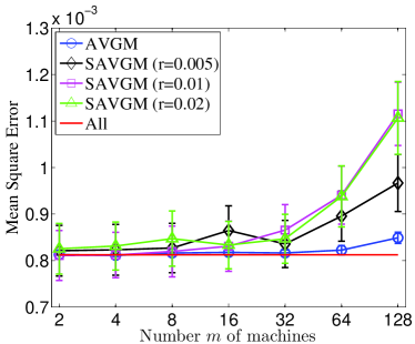
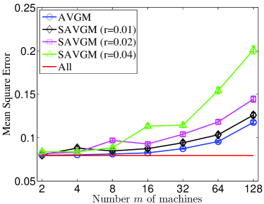
(a) $d=20$	(b) $d=200$

Figure 3: The error $\|{\widehat{\theta}-\theta^{*}}\|_{2}^{2}$ plotted against the number of machines $m$ for the Avgm and Savgm methods, with standard errors across twenty simulations, using the normal regression model (22a). The oracle estimator is denoted by the line “All.”

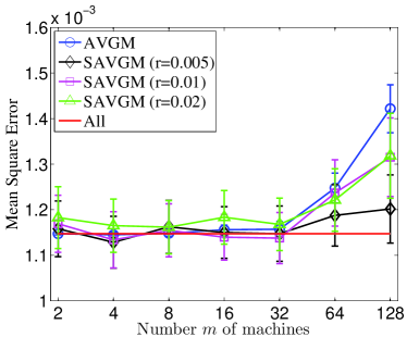
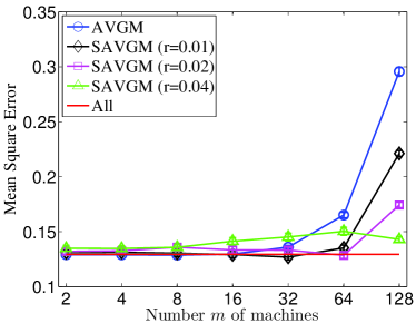
(a) $d=20$	(b) $d=200$

Figure 4: The error $\|{\widehat{\theta}-\theta^{*}}\|_{2}^{2}$ plotted against the number of machines $m$ for the Avgm and Savgm methods, with standard errors across twenty simulations, using the non-normal regression model (22c). The oracle estimator is denoted by the line “All.”

We now turn to developing an understanding of the Savgm algorithm in comparison to the standard average mixture algorithm, developing intuition for the benefits and drawbacks of the method. Before describing the results, we remark that for the standard regression model (22a), the least-squares solution is unbiased for $\theta^{*}$, so we expect subsampled averaging to yield little (if any) improvement. The Savgm method is essentially aimed at correcting the bias of the estimator $\overline{\theta}_{1}$, and de-biasing an unbiased estimator only increases its variance. However, for the mis-specified models (22b) and (22c) we expect to see some performance gains. In our experiments, we use multiple sub-sampling rates to study their effects, choosing $\ratio\in\{0.005,0.01,0.02,0.04\}$, where we recall that the output of the Savgm algorithm is the vector $\widehat{\theta}:=(\overline{\theta}_{1}-\ratio\overline{\theta}_{2})/(1-\ratio)$.

We begin with experiments in which the data is generated as in the previous section. That is, to generate a feature vector $x\in{}^{d}$, choose five distinct indices in $\{1,\ldots,d\}$ uniformly at random, and the entries of $x$ at those indices are distributed as $N(0,1)$. In Figure 3, we plot the results of simulations comparing Avgm and Savgm with data generated from the normal regression model (22a). Both algorithms have have low error rates, but the Avgm method is slightly better than the Savgm method for both values of the dimension $d$ and all and sub-sampling rates . As expected, in this case the Savgm method does not offer improvement over Avgm, since the estimators are unbiased. (In Figure 3(a), we note that the standard error is in fact very small, since the mean-squared error is only of order $10^{-3}$.)

To understand settings in which subsampling for bias correction helps, in Figure 4, we plot mean-square error curves for the least-squares regression problem when the vector $y$ is sampled according to the non-normal regression model (22c). In this case, the least-squares estimator is biased for $\theta^{*}$ (which, as before, we estimate by solving a larger regression problem using $10N$ data samples). Figure 4 shows that both the Avgm and Savgm method still enjoy good performance; in some cases, the Savgm method even beats the oracle least-squares estimator for $\theta^{*}$ that uses all $N$ samples. Since the Avgm estimate is biased in this case, its error curve increases roughly quadratically with $m$, which agrees with our theoretical predictions in Theorem 1. In contrast, we see that the Savgm algorithm enjoys somewhat more stable performance, with increasing benefit as the number of machines $m$ increases. For example, in case of $d=200$, if we choose $\ratio=0.01$ for $m\leq 32$, choose $\ratio=0.02$ for $m=64$ and $\ratio=0.04$ for $m=128$, then Savgm has performance comparable with the oracle method that uses all $N$ samples. Moreover, we see that all the values of —at least for the reasonably small values we use in the experiment—provide performance improvements over a non-subsampled distributed estimator.

For our final simulation, we plot results comparing Savgm with Avgm in model (22b), which is mis-specified but still a normal model. We use a simpler data generating mechanism, specifically, we draw $x\sim N(0,I_{d\times d})$ from a standard $d$-dimensional normal, and $v$ is chosen uniformly in $[0,1]$; in this case, the population minimizer has the closed form $\theta^{*}=u+3v$. Figure 5 shows the results for dimensions $d=20$ and $d=40$ performed over $100$ experiments (the standard errors are too small to see). Since the model (22b) is not that badly mis-specified, the performance of the Savgm method improves upon that of the Avgm method only for relatively large values of $m$, however, the performance of the Savgm is always at least as good as that of Avgm.

\psfrag{Avgm}{\small{{Avgm}}}\psfrag{SAvgm (r=(d/n) 2/3)--}{\small{{Savgm}\ $(\ratio=(d/n)^{2/3})$}}\includegraphics[width=195.12767pt]{Images/mse-20}	\psfrag{Avgm}{\small{{Avgm}}}\psfrag{SAvgm (r=(d/n) 2/3)--}{\small{{Savgm}\ $(\ratio=(d/n)^{2/3})$}}\includegraphics[width=195.12767pt]{Images/mse-40}
(a) $d=20$	(b) $d=40$

Figure 5: The error $\|{\widehat{\theta}-\theta^{*}}\|_{2}^{2}$ plotted against the number of machines $m$ for the Avgm and Savgm methods using regression model (22b).

5 Experiments with advertising data

Table 1: Features used in online advertisement prediction problem.

Feature Name	Dimension	Description
Query	20000	Word tokens appearing in the query.
Gender	3	Gender of the user
Keyword	20000	Word tokens appearing in the purchase keywords.
Title	20000	Word tokens appearing in the ad title.
Advertiser	39191	Advertiser’s ID
AdID	641707	Advertisement’s ID.
Age	6	Age of the user
UserFreq	25	Number of appearances of the same user.
Position	3	Position of advertisement on search page.
Depth	3	Number of ads in the session.
QueryFreq	25	Number of occurrences of the same query.
AdFreq	25	Number of occurrences of the same ad.
QueryLength	20	Number of words in the query.
TitleLength	30	Number of words in the ad title.
DespLength	50	Number of words in the ad description.
QueryCtr	150	Average click-through-rate for query.
UserCtr	150	Average click-through-rate for user.
AdvrCtr	150	Average click-through-rate for advertiser.
WordCtr	150	Average click-through-rate for keyword advertised.
UserAdFreq	20	Number of times this user sees an ad.
UserQueryFreq	20	Number of times this user performs a search.

Predicting whether a user of a search engine will click on an advertisement presented to him or her is of central importance to the business of several internet companies, and in this section, we present experiments studying the performance of the Avgm and Savgm methods for this task. We use a large dataset from the Tencent search engine, soso.com (Sun, 2012), which contains 641,707 distinct advertisement items with $N=235,\!582,\!879$ data samples.

Each sample consists of a so-called impression, which in the terminology of the information retrieval literature (e.g., see the book by Manning et al. (2008)), is a list containing a user-issued search, the advertisement presented to the user in response to the search, and a label $y\in\{+1,-1\}$ indicating whether the user clicked on the advertisement. The ads in our dataset were presented to 23,669,283 distinct users.

Transforming an impression into a useable set of regressors $x$ is non-trivial, but the Tencent dataset provides a standard encoding. We list the features present in the data in Table 1, along with some description of their meaning. Each text-based feature—that is, those made up of words, which are Query, Keyword, and Title—is given a “bag-of-words” encoding (Manning et al., 2008). This encoding assigns each of 20,000 possible words an index, and if the word appears in the query (or Keyword or Title feature), the corresponding index in the vector $x$ is set to 1. Words that do not appear are encoded with a zero. Real-valued features, corresponding to the bottom fifteen features in Table 1 beginning with “Age”, are binned into a fixed number of intervals $[-\infty,a_{1}],\left({a_{1}},{a_{2}}\right],\ldots,\left({a_{k}},{\infty}\right]$, each of which is assigned an index in $x$. (Note that the intervals and number thereof vary per feature, and the dimension of the features listed in Table 1 corresponds to the number of intervals). When a feature falls into a particular bin, the corresponding entry of $x$ is assigned a 1, and otherwise the entries of $x$ corresponding to the feature are 0. Each feature has one additional value for “unknown.” The remaining categorical features—gender, advertiser, and advertisement ID (AdID)—are also given $\{0,1\}$ encodings, where only one index of $x$ corresponding to the feature may be non-zero (which indicates the particular gender, advertiser, or AdID). This combination of encodings yields a binary-valued covariate vector $x\in\{0,1\}^{d}$ with $d=741,\!725$ dimensions. Note also that the features incorporate information about the user, advertisement, and query issued, encoding information about their interactions into the model.

Our goal is to predict the probability of a user clicking a given advertisement as a function of the covariates in Table 1. To do so, we use a logistic regression model to estimate the probability of a click response

$$P(y=1\mid x;\theta):=\frac{1}{1+\exp(-\left\langle\theta,x\right\rangle)},$$

where $\theta\in\mathbb{R}^{d}$ is the unknown regression vector. We use the negative logarithm of $P$ as the loss, incorporating a ridge regularization penalty. This combination yields instantaneous loss

$$f(\theta;(x,y))=\log\left(1+\exp(-y\left\langle\theta,x\right\rangle)\right)+\frac{\lambda}{2}\left\|{\theta}\right\|_{2}^{2}.$$ (23)

In all our experiments, we assume that the population negative log-likelihood risk has local strong convexity as suggested by Assumption B. In practice, we use a small regularization parameter $\lambda=10^{-6}$ to ensure fast convergence for the local sub-problems.

\psfrag{AVGM}{\small{{Avgm}}}\psfrag{BAVGM $r=0.1$}{\small{{Savgm}\ ($\ratio=.1$)}}\psfrag{BAVGM $r=0.25$}{\small{{Savgm}\ ($\ratio=.25$)}}\includegraphics[width=195.12767pt]{Images/soso_comparison}
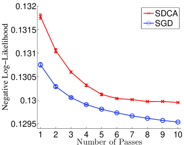
(a)	(b)

Figure 6: The negative log-likelihood of the output of the Avgm, Savgm, and stochastic methods on the held-out dataset for the click-through prediction task. (a) Performance of the Avgm and Savgm methods versus the number of splits $m$ of the data. (b) Performance of SDCA and SGD baselines as a function of number of passes through the entire dataset.

For this problem, we cannot evaluate the mean-squared error $\|{\widehat{\theta}-\theta^{*}}\|_{2}^{2}$, as we do not know the true optimal parameter $\theta^{*}$. Consequently, we evaluate the performance of an estimate $\widehat{\theta}$ using log-loss on a held-out dataset. Specifically, we perform a five-fold validation experiment, where we shuffle the data and partition it into five equal-sized subsets. For each of our five experiments, we hold out one partition to use as the test set, using the remaining data as the training set for inference. When studying the Avgm or Savgm method, we compute the local estimate $\theta_{i}$ via a trust-region Newton-based method (Nocedal and Wright, 2006) implemented by LIBSVM (Chang and Lin, 2011).

The dataset is too large to fit in the memory of most computers: in total, four splits of the data require 55 gigabytes. Consequently, it is difficult to provide an oracle training comparison using the full $N$ samples. Instead, for each experiment, we perform 10 passes of stochastic dual coordinate ascent (SDCA) (Shalev-Shwartz and Zhang, 2012) and 10 passes of stochastic gradient descent (SGD) through the dataset to get two rough baselines of the performance attained by the empirical minimizer for the entire training dataset. Figure 6(b) shows the hold-out set log-loss after each of the sequential passes through the training data finishes. Note that although the SDCA enjoys faster convergence rate on the regularized empirical risk (Shalev-Shwartz and Zhang, 2012), the plot shows that the SGD has better generalization performance.

In Figure 6(a), we show the average hold-out set log-loss (with standard errors) of the estimator $\overline{\theta}_{1}$ provided by the Avgm method versus number of splits of the data $m$, and we also plot the log-loss of the Savgm method using subsampling ratios of $\ratio\in\{.1,.25\}$. The plot shows that for small $m$, both Avgm and Savgm enjoy good performance, comparable to or better than (our proxy for) the oracle solution using all $N$ samples. As the number of machines $m$ grows, however, the de-biasing provided by the subsampled bootstrap method yields substantial improvements over the standard Avgm method. In addition, even with $m=128$ splits of the dataset, the Savgm method gives better hold-out set performance than performing two passes of stochastic gradient on the entire dataset of $m$ samples; with $m=64$, Savgm enjoys performance as strong as looping through the data four times with stochastic gradient descent. This is striking, since doing even one pass through the data with stochastic gradient descent gives minimax optimal convergence rates (Polyak and Juditsky, 1992; Agarwal et al., 2012). In ranking applications, rather than measuring negative log-likelihood, one may wish to use a direct measure of prediction error; to that end, Figure 7 shows plots of the area-under-the-curve (AUC) measure for the Avgm and Savgm methods; AUC is a well-known measure of prediction error for bipartite ranking (Manning et al., 2008). Broadly, this plot shows a similar story to that in Figure 6.

\psfrag{AVGM}{{Avgm}}\psfrag{BAVGM $r=0.1$}{{Savgm}\ $(r=.1)$}\psfrag{BAVGM $r=0.25$}{{Savgm}\ $(r=.25)$}\includegraphics[width=216.81pt]{Images/soso_comparison_auc}

Figure 7: The area-under-the-curve (AUC) measure of ranking error for the output of the Avgm and Savgm methods for the click-through prediction task.

\psfrag{BAVGM $m=128$}{\small{{Savgm}\ $(m=128)$}}\includegraphics[width=195.12767pt]{Images/soso_r_compare}

Figure 8: The log-loss on held-out data for the Savgm method applied with $m=128$ parallel splits of the data, plotted versus the sub-sampling rate .

It is instructive and important to understand the sensitivity of the Savgm method to the value of the resampling parameter . We explore this question in Figure 8 using $m=128$ splits, where we plot the log-loss of the Savgm estimator on the held-out data set versus the subsampling ratio . We choose $m=128$ because more data splits provide more variable performance in . For the soso.com ad prediction data set, the choice $\ratio=.25$ achieves the best performance, but Figure 8 suggests that mis-specifying the ratio is not terribly detrimental. Indeed, while the performance of Savgm degrades to that of the Avgm method, a wide range of settings of give improved performance, and there does not appear to be a phase transition to poor performance.

6 Discussion

Large scale statistical inference problems are challenging, and the difficulty of solving them will only grow as data becomes more abundant: the amount of data we collect is growing much faster than the speed or storage capabilities of our computers. Our Avgm, Savgm, and SGDavgm methods provide strategies for efficiently solving such large-scale risk minimization problems, enjoying performance comparable to an oracle method that is able to access the entire large dataset. We believe there are several interesting questions that remain open after this work. First, nonparametric estimation problems, which often suffer superlinear scaling in the size of the data, may provide an interesting avenue for further study of decomposition-based methods. Our own recent work has addressed aspects of this challenge in the context of kernel methods for non-parametric regression (Zhang et al., 2013). More generally, an understanding of the interplay between statistical efficiency and communication could provide an avenue for further research, and it may also be interesting to study the effects of subsampled or bootstrap-based estimators in other distributed environments.

Acknowledgments

We thank Joel Tropp for some informative discussions on and references for matrix concentration and moment inequalities. We also thank Ohad Shamir for pointing out a mistake in the statements of results related to Theorem 1, and the editor and reviewers for their helpful comments and feedback. JCD was supported by the Department of Defence under the NDSEG Fellowship Program and by a Facebook PhD fellowship. This work was partially funded by Office of Naval Research MURI grant N00014-11-1-0688 to MJW.

A The necessity of smoothness

Here we show that some version of the smoothness conditions presented in Assumption C are necessary for averaging methods to attain better mean-squared error than using only the $n$ samples on a single processor. Given the loss function (10), let $n_{0}=\sum_{i=1}^{n}1_{\left({X_{i}=0}\right)}$ to be the count of 0 samples. Using $\theta_{1}$ as shorthand for $\theta_{1,i}$, we see by inspection that the empirical minimizer $\theta_{1}$ is

$$\theta_{1}=\begin{cases}\frac{n_{0}}{n}-\frac{1}{2}&\mbox{when}~{}n_{0}\leq n/2\\ 1-\frac{n}{2n_{0}}&\mbox{otherwise.}\end{cases}$$

For simplicity, we may assume that $n$ is odd. In this case, we obtain that

$$\mathbb{E}[\theta_{1}] =\frac{1}{4}+\mathbb{E}\left[\frac{n_{0}}{n}1_{\left({n_{0}<n/2}\right)}\right]-\mathbb{E}\left[\frac{n}{2n_{0}}1_{\left({n_{0}>n/2}\right)}\right]$$

$$=\frac{1}{4}+\frac{1}{2^{n}}\sum_{i=0}^{\left\lfloor{n/2}\right\rfloor}\binom{n}{i}\frac{i}{n}-\frac{1}{2^{n}}\sum_{i=\left\lceil{n/2}\right\rceil}^{n}\binom{n}{i}\frac{n}{2i}=\frac{1}{4}+\frac{1}{2^{n}}\sum_{i=0}^{\left\lfloor{n/2}\right\rfloor}\binom{n}{i}\left[\frac{i}{n}-\frac{n}{2(n-i)}\right]$$

by the symmetry of the binomial. Adding and subtracting $\frac{1}{2}$ from the term within the braces, noting that $P(n_{0}<n/2)=1/2$, we have the equality

$$\mathbb{E}[\theta_{1}]=\frac{1}{2^{n}}\sum_{i=0}^{\left\lfloor{n/2}\right\rfloor}\binom{n}{i}\left[\frac{i}{n}-\frac{n}{2(n-i)}+\frac{1}{2}\right]=\frac{1}{2^{n}}\sum_{i=0}^{\left\lfloor{n/2}\right\rfloor}\binom{n}{i}\frac{i(n-2i)}{2n(n-i)}.$$

If $Z$ is distributed normally with mean $1/2$ and variance $1/(4n)$, then an asymptotic expansion of the binomial distribution yields

$$\left(\frac{1}{2}\right)^{n}\sum_{i=0}^{\left\lfloor{n/2}\right\rfloor}\binom{n}{i}\frac{i(n-2i)}{2n(n-i)} =\mathbb{E}\left[\frac{Z(1-2Z)}{2-2Z}\mid 0\leq Z\leq\frac{1}{2}\right]+o(n^{-1/2})$$

$$\geq\frac{1}{2}\mathbb{E}\left[Z-2Z^{2}\mid 0\leq Z\leq\frac{1}{2}\right]+o(n^{-1/2})=\Omega(n^{-\frac{1}{2}}),$$

the final equality following from standard calculations, since $\mathbb{E}[|Z|]=\Omega(n^{-1/2})$.

B Proof of Theorem 1

Although Theorem 1 is in terms of bounds on $8^{th}$ order moments, we prove a somewhat more general result in terms of a set of $({k_{0}},{k_{1}},{k_{2}})$ moment conditions given by

$$\mathbb{E}[\left\|{\nabla f(\theta;X)}\right\|_{2}^{k_{0}}]\leq G^{k_{0}},\qquad~{}~{}~{}\mathbb{E}[\left|\!\left|\!\left|{\nabla^{2}f(\theta;X)-\nabla^{2}F_{0}(\theta)}\right|\!\right|\!\right|_{2}^{k_{1}}]\leq H^{k_{1}},$$

$$\mathbb{E}[L(X)^{k_{2}}]\leq L^{k_{2}}\quad\mbox{and}\quad\mathbb{E}[(L(X)-\mathbb{E}[L(X)])^{k_{2}}]\leq L^{k_{2}}$$

for $\theta\in U$. (Recall the definition of $U$ prior to Assumption C). Doing so allows sharper control if higher moment bounds are available. The reader should recall throughout our arguments that we have assumed $\min\{{k_{0}},{k_{1}},{k_{2}}\}\geq 8$. Throughout the proof, we use $F_{1}$ and $\theta_{1}$ to indicate the local empirical objective and empirical minimizer of machine $1$ (which have the same distribution as those of the other processors), and we recall the notation $1_{\left({\mathcal{E}}\right)}$ for the indicator function of the event $\mathcal{E}$.

Before beginning the proof of Theorem 1 proper, we begin with a simple inequality that relates the error term $\overline{\theta}-\theta^{*}$ to an average of the errors $\theta_{i}-\theta^{*}$, each of which we can bound in turn. Specifically, a bit of algebra gives us that

$$\mathbb{E}[\left\|{\overline{\theta}-\theta^{*}}\right\|_{2}^{2}] =\mathbb{E}\bigg{[}\bigg{\|}{\frac{1}{m}\sum_{i=1}^{m}\theta_{i}-\theta^{*}}\bigg{\|}_{2}^{2}\bigg{]}$$

$$=\frac{1}{m^{2}}\sum_{i=1}^{m}\mathbb{E}[\left\|{\theta_{i}-\theta^{*}}\right\|_{2}^{2}]+\frac{1}{m^{2}}\sum_{i\neq j}\mathbb{E}[\left\langle\theta_{i}-\theta^{*},\theta_{j}-\theta^{*}\right\rangle]$$

$$\leq\frac{1}{m}\mathbb{E}[\left\|{\theta_{1}-\theta^{*}}\right\|_{2}^{2}]+\frac{m(m-1)}{m^{2}}\left\|{\mathbb{E}[\theta_{1}-\theta^{*}]}\right\|_{2}^{2}$$

$$\leq\frac{1}{m}\mathbb{E}[\left\|{\theta_{1}-\theta^{*}}\right\|_{2}^{2}]+\left\|{\mathbb{E}[\theta_{1}-\theta^{*}]}\right\|_{2}^{2}.$$ (24)

Here we used the definition of the averaged vector $\overline{\theta}$ and the fact that for $i\neq j$, the vectors $\theta_{i}$ and $\theta_{j}$ are statistically independent, they are functions of independent samples. The upper bound (24) illuminates the path for the remainder of our proof: we bound each of $\mathbb{E}[\left\|{\theta_{i}-\theta^{*}}\right\|_{2}^{2}]$ and $\left\|{\mathbb{E}[\theta_{i}-\theta^{*}]}\right\|_{2}^{2}$. Intuitively, since our objective is locally strongly convex by Assumption B, the empirical minimizing vector $\theta_{1}$ is a nearly unbiased estimator for $\theta^{*}$, which allows us to prove the convergence rates in the theorem.

We begin by defining three events—which we (later) show hold with high probability—that guarantee the closeness of $\theta_{1}$ and $\theta^{*}$. In rough terms, when these events hold, the function $F_{1}$ behaves similarly to the population risk $F_{0}$ around the point $\theta^{*}$; since $F_{0}$ is locally strongly convex, the minimizer $\theta_{1}$ of $F_{1}$ will be close to $\theta^{*}$. Recall that Assumption C guarantees the existence of a ball $U_{\rho}=\{\theta\in\mathbb{R}^{d}:\left\|{\theta-\theta^{*}}\right\|_{2}<\rho\}$ of radius $\rho\in(0,1)$ such that

$$\left|\!\left|\!\left|{\nabla^{2}f(\theta;x)-\nabla^{2}f(\theta^{\prime};x)}\right|\!\right|\!\right|_{2}\leq L(x)\left\|{\theta-\theta^{\prime}}\right\|_{2}$$

for all $\theta,\theta^{\prime}\in U_{\rho}$ and any $x$, where $\mathbb{E}[L(X)^{k_{2}}]\leq L^{k_{2}}$. In addition, Assumption B guarantees that $\nabla^{2}F_{0}(\theta^{*})\succeq\lambda I$. Now, choosing the potentially smaller radius $\delta_{\rho}=\min\{\rho,\rho\lambda/4L\}$, we can define the three “good” events

$$\mathcal{E}_{0} :=\bigg{\{}\frac{1}{n}\sum_{i=1}^{n}L(X_{i})\leq 2L\bigg{\}},$$

$$\mathcal{E}_{1} :=\left\{\left|\!\left|\!\left|{\nabla^{2}F_{1}(\theta^{*})-\nabla^{2}F_{0}(\theta^{*})}\right|\!\right|\!\right|_{2}\leq\frac{\rho\lambda}{2}\right\},\quad\mbox{and}$$ (25)

$$\mathcal{E}_{2} :=\left\{\left\|{\nabla F_{1}(\theta^{*})}\right\|_{2}\leq\frac{(1-\rho)\lambda\delta_{\rho}}{2}\right\}.$$

We then have the following lemma:

Lemma 6

Under the events $\mathcal{E}_{0}$, $\mathcal{E}_{1}$, and $\mathcal{E}_{2}$ previously defined (25), we have

$$\left\|{\theta_{1}-\theta^{*}}\right\|_{2}\leq\frac{2\left\|{\nabla F_{1}(\theta^{*})}\right\|_{2}}{(1-\rho)\lambda},\quad\mbox{and}\quad\nabla^{2}F_{1}(\theta)\succeq(1-\rho)\lambda I_{d\times d}.$$

The proof of Lemma 6 relies on some standard optimization guarantees relating gradients to minimizers of functions (e.g. Boyd and Vandenberghe (2004), Chapter 9), although some care is required since smoothness and strong convexity hold only locally in our problem. As the argument is somewhat technical, we defer it to Appendix E.

Our approach from here is to give bounds on $\mathbb{E}[\left\|{\theta_{1}-\theta^{*}}\right\|_{2}^{2}]$ and $\left\|{\mathbb{E}[\theta_{1}-\theta^{*}]}\right\|_{2}^{2}$ by careful Taylor expansions, which allows us to bound $\mathbb{E}[\left\|{\overline{\theta}_{1}-\theta^{*}}\right\|_{2}^{2}]$ via our initial expansion (24). We begin by noting that whenever the events $\mathcal{E}_{0}$, $\mathcal{E}_{1}$, and $\mathcal{E}_{2}$ hold, then $\nabla F_{1}(\theta_{1})=0$, and moreover, by a Taylor series expansion of $\nabla F_{1}$ between $\theta^{*}$ and $\theta_{1}$, we have

$$0=\nabla F_{1}(\theta_{1}) =\nabla F_{1}(\theta^{*})+\nabla^{2}F_{1}(\theta^{\prime})(\theta_{1}-\theta^{*})$$

where $\theta^{\prime}=\kappa\theta^{*}+(1-\kappa)\theta_{1}$ for some $\kappa\in[0,1]$. By adding and subtracting terms, we have

$$0=\nabla F_{1}(\theta^{*})+(\nabla^{2}F_{1}(\theta^{\prime})-\nabla^{2}F_{1}(\theta^{*}))(\theta_{1}-\theta^{*})\\ +(\nabla^{2}F_{1}(\theta^{*})-\nabla^{2}F_{0}(\theta^{*}))(\theta_{1}-\theta^{*})+\nabla^{2}F_{0}(\theta^{*})(\theta_{1}-\theta^{*}).$$ (26)

Since $\nabla^{2}F_{0}(\theta^{*})\succeq\lambda I$, we can define the inverse Hessian matrix $\Sigma^{-1}:=[\nabla^{2}F_{0}(\theta^{*})]^{-1}$, and setting $\Delta:=\theta_{1}-\theta^{*}$, we multiply both sides of the Taylor expansion (26) by $\Sigma^{-1}$ to obtain the relation

$$\Delta=-\Sigma^{-1}\nabla F_{1}(\theta^{*})+\Sigma^{-1}(\nabla^{2}F_{1}(\theta^{*})-\nabla^{2}F_{1}(\theta^{\prime}))\Delta+\Sigma^{-1}(\nabla^{2}F_{0}(\theta^{*})-\nabla^{2}F_{1}(\theta^{*}))\Delta.$$ (27)

Thus, if we define the matrices $P=\nabla^{2}F_{0}(\theta^{*})-\nabla^{2}F_{1}(\theta^{*})$ and $Q=\nabla^{2}F_{1}(\theta^{*})-\nabla^{2}F_{1}(\theta^{\prime})$, equality (27) can be re-written as

$$\theta_{1}-\theta^{*}=-\Sigma^{-1}\nabla F_{1}(\theta^{*})+\Sigma^{-1}(P+Q)(\theta_{1}-\theta^{*}).$$ (28)

Note that equation (28) holds when the conditions of Lemma 6 hold, and otherwise we may simply assert only that $\left\|{\theta_{1}-\theta^{*}}\right\|_{2}\leq R$. Roughly, we expect the final two terms in the error expansion (28) to be of smaller order than the first term, since we hope that $\theta_{1}-\theta^{*}\rightarrow 0$ and additionally that the Hessian differences decrease to zero at a sufficiently fast rate. We now formalize this intuition.

Inspecting the Taylor expansion (28), we see that there are several terms of a form similar to $(\nabla^{2}F_{0}(\theta^{*})-\nabla^{2}F_{1}(\theta^{*}))(\theta_{1}-\theta^{*})$; using the smoothness Assumption C, we can convert these terms into higher order terms involving only $\theta_{1}-\theta^{*}$. Thus, to effectively control the expansions (27) and (28), we must show that higher order terms of the form $\mathbb{E}[\left\|{\theta_{1}-\theta^{*}}\right\|_{2}^{k}]$, for $k\geq 2$, decrease quickly enough in $n$.

Control of $\mathbb{E}[\left\|{\theta_{1}-\theta^{*}}\right\|_{2}^{k}]$:

Recalling the events (25), we define $\mathcal{E}:=\mathcal{E}_{0}\cap\mathcal{E}_{1}\cap\mathcal{E}_{2}$ and then observe that

$$\mathbb{E}[\left\|{\theta_{1}-\theta^{*}}\right\|_{2}^{k}] =\mathbb{E}[1_{\left({\mathcal{E}}\right)}\left\|{\theta_{1}-\theta^{*}}\right\|_{2}^{k}]+\mathbb{E}[1_{\left({\mathcal{E}^{c}}\right)}\left\|{\theta_{1}-\theta^{*}}\right\|_{2}^{k}]$$

$$\leq\frac{2^{k}\mathbb{E}[1_{\left({\mathcal{E}}\right)}\left\|{\nabla F_{1}(\theta^{*})}\right\|_{2}^{k}]}{(1-\rho)^{k}\lambda^{k}}+\mathbb{P}(\mathcal{E}^{c})R^{k}$$

$$\leq\frac{2^{k}\mathbb{E}[\left\|{\nabla F_{1}(\theta^{*})}\right\|_{2}^{k}]}{(1-\rho)^{k}\lambda^{k}}+\mathbb{P}(\mathcal{E}^{c})R^{k},$$

where we have used the bound $\left\|{\theta-\theta^{*}}\right\|_{2}\leq R$ for all $\theta\in\Theta$, from Assumption A. Our goal is to prove that $\mathbb{E}[\left\|{\nabla F_{1}(\theta^{*})}\right\|_{2}^{k}]=\mathcal{O}(n^{-k/2})$ and that $\mathbb{P}(\mathcal{E}^{c})=\mathcal{O}(n^{-k/2})$. We move forward with a two lemmas that lay the groundwork for proving these two facts:

Lemma 7

Under Assumption C, there exist constants $C$ and $C^{\prime}$ (dependent only on the moments ${k_{0}}$ and ${k_{1}}$ respectively) such that

$$\mathbb{E}[\left\|{\nabla F_{1}(\theta^{*})}\right\|_{2}^{k_{0}}] \leq C\frac{G^{k_{0}}}{n^{{k_{0}}/2}},~{}~{}~{}\mbox{and}$$ (29a)

$$\mathbb{E}[\left|\!\left|\!\left|{\nabla^{2}F_{1}(\theta^{*})-\nabla^{2}F_{0}(\theta^{*})}\right|\!\right|\!\right|_{2}^{k_{1}}] \leq C^{\prime}\frac{\log^{{k_{1}}/2}(2d)H^{k_{1}}}{n^{{k_{1}}/2}}.$$ (29b)

See Appendix F for the proof of this claim.

As an immediate consequence of Lemma 7, we see that the events $\mathcal{E}_{1}$ and $\mathcal{E}_{2}$ defined by (25) occur with reasonably high probability. Indeed, recalling that $\mathcal{E}=\mathcal{E}_{0}\cap\mathcal{E}_{1}\cap\mathcal{E}_{2}$, Boole’s law and the union bound imply

$$\mathbb{P}(\mathcal{E}^{c})=\mathbb{P}(\mathcal{E}_{0}^{c}\cup\mathcal{E}_{1}^{c}\cup\mathcal{E}_{2}^{c})$$

$$\leq\mathbb{P}(\mathcal{E}_{0}^{c})+\mathbb{P}(\mathcal{E}_{1}^{c})+\mathbb{P}(\mathcal{E}_{2}^{c})$$

$$\leq\frac{\mathbb{E}[|\frac{1}{n}\sum_{i=1}^{n}L(X_{i})-\mathbb{E}[L(X)]|^{k_{2}}]}{L^{k_{2}}}+\frac{2^{k_{1}}\mathbb{E}[\left|\!\left|\!\left|{\nabla^{2}F_{1}(\theta^{*})-\nabla^{2}F_{0}(\theta^{*})}\right|\!\right|\!\right|_{2}^{k_{1}}]}{\rho^{k_{1}}\lambda^{k_{1}}}+\frac{2^{k_{0}}\mathbb{E}[\left\|{\nabla F_{1}(\theta^{*})}\right\|_{2}^{k_{0}}]}{(1-\rho)^{k_{0}}\lambda^{k_{0}}\delta_{\rho}^{k_{0}}}$$

$$\leq C_{2}\frac{1}{n^{{k_{2}}/2}}+C_{1}\frac{\log^{{k_{1}}/2}(2d)H^{k_{1}}}{n^{{k_{1}}/2}}+C_{0}\frac{G^{k_{0}}}{n^{{k_{0}}/2}}$$ (30)

for some universal constants $C_{0},C_{1},C_{2}$, where in the second-to-last line we have invoked the moment bound in Assumption C. Consequently, we find that

$$\mathbb{P}(\mathcal{E}^{c})R^{k}=\mathcal{O}(R^{k}(n^{-{k_{1}}/2}+n^{-{k_{2}}/2}+n^{-{k_{0}}/2})\quad\mbox{for any $k\in\mathbb{N}$.}$$

In summary, we have proved the following lemma:

Lemma 8

Let Assumptions B and C hold. For any $k\in\mathbb{N}$ with $k\leq\min\{{k_{0}},{k_{1}},{k_{2}}\}$, we have

$$\mathbb{E}[\left\|{\theta_{1}-\theta^{*}}\right\|_{2}^{k}]=\mathcal{O}\left(n^{-k/2}\cdot\frac{G^{k}}{(1-\rho)^{k}\lambda^{k}}+n^{-{k_{0}}/2}+n^{-{k_{1}}/2}+n^{-{k_{2}}/2}\right)=\mathcal{O}\left(n^{-k/2}\right),$$

where the order statements hold as $n\rightarrow+\infty$.

Now recall the matrix $Q=\nabla^{2}F_{1}(\theta^{*})-\nabla^{2}F_{1}(\theta^{\prime})$ defined following equation (27). The following result controls the moments of its operator norm:

Lemma 9

For $k\leq\min\{{k_{2}},{k_{1}},{k_{0}}\}/2$, we have $\mathbb{E}[\left|\!\left|\!\left|{Q}\right|\!\right|\!\right|_{2}^{k}]=\mathcal{O}(n^{-k/2})$.

Proof: We begin by using Jensen’s inequality and Assumption C to see that

$$\left|\!\left|\!\left|{Q}\right|\!\right|\!\right|^{k}\leq\frac{1}{n}\sum_{i=1}^{n}\left|\!\left|\!\left|{\nabla^{2}f(\theta^{\prime};X_{i})-\nabla^{2}f(\theta^{*};X_{i})}\right|\!\right|\!\right|^{k}\leq\frac{1}{n}\sum_{i=1}^{n}L(X_{i})^{k}\left\|{\theta^{\prime}-\theta^{*}}\right\|_{2}^{k}.$$

Now we apply the Cauchy-Schwarz inequality and Lemma 8, thereby obtaining

$$\mathbb{E}[\left|\!\left|\!\left|{Q}\right|\!\right|\!\right|_{2}^{k}]\leq\mathbb{E}\left[\bigg{(}\frac{1}{n}\sum_{i=1}^{n}L(X_{i})^{k}\bigg{)}^{2}\right]^{\frac{1}{2}}\mathbb{E}\left[\left\|{\theta_{1}-\theta^{*}}\right\|_{2}^{2k}\right]^{\frac{1}{2}}=\mathcal{O}\left(L^{k}\frac{G^{k}}{(1-\rho)^{k}\lambda^{k}}n^{-k/2}\right),$$

where we have used Assumption C again.  

Lemma 8 allows us to control the first term from our initial bound (24) almost immediately. Indeed, using our last Taylor expansion (28) and the definition of the event $\mathcal{E}=\mathcal{E}_{0}\cap\mathcal{E}_{1}\cap\mathcal{E}_{2}$, we have

$$\mathbb{E}[\left\|{\theta_{1}-\theta^{*}}\right\|_{2}^{2}] =\mathbb{E}\left[1_{\left({\mathcal{E}}\right)}\left\|{-\Sigma^{-1}\nabla F_{1}(\theta^{*})+\Sigma^{-1}(P+Q)(\theta_{1}-\theta^{*})}\right\|_{2}^{2}\right]+\mathbb{E}[1_{\left({\mathcal{E}^{c}}\right)}\left\|{\theta_{1}-\theta^{*}}\right\|_{2}^{2}]$$

$$\leq 2\mathbb{E}\left[\left\|{\Sigma^{-1}\nabla F_{1}(\theta^{*})}\right\|_{2}^{2}\right]+2\mathbb{E}\left[\left\|{\Sigma^{-1}(P+Q)(\theta_{1}-\theta^{*})}\right\|_{2}^{2}\right]+\mathbb{P}(\mathcal{E}^{c})R^{2},$$

where we have applied the inequality $(a+b)^{2}\leq 2a^{2}+2b^{2}$. Again using this same inequality, then applying Cauchy-Schwarz and Lemmas 8 and 9, we see that

$$\mathbb{E}\left[\left\|{\Sigma^{-1}(P+Q)(\theta_{1}-\theta^{*})}\right\|_{2}^{2}\right]\leq 2\left|\!\left|\!\left|{\Sigma^{-1}}\right|\!\right|\!\right|_{2}^{2}\left(\mathbb{E}[\left|\!\left|\!\left|{P}\right|\!\right|\!\right|_{2}^{2}\left\|{\theta_{1}-\theta^{*}}\right\|_{2}^{2}]+\mathbb{E}[\left|\!\left|\!\left|{Q}\right|\!\right|\!\right|_{2}^{2}\left\|{\theta_{1}-\theta^{*}}\right\|_{2}^{2}]\right)$$

$$\qquad\qquad\qquad\qquad\quad~{}\leq 2\left|\!\left|\!\left|{\Sigma^{-1}}\right|\!\right|\!\right|_{2}^{2}\left(\sqrt{\mathbb{E}[\left|\!\left|\!\left|{P}\right|\!\right|\!\right|_{2}^{4}]\mathbb{E}[\left\|{\theta_{1}-\theta^{*}}\right\|_{2}^{4}]}+\sqrt{\mathbb{E}[\left|\!\left|\!\left|{Q}\right|\!\right|\!\right|_{2}^{4}]\mathbb{E}[\left\|{\theta_{1}-\theta^{*}}\right\|_{2}^{4}]}\right)$$

$$\qquad\qquad\qquad\qquad\quad~{}=\mathcal{O}(n^{-2}),$$

where we have used the fact that $\min\{{k_{0}},{k_{1}},{k_{2}}\}\geq 8$ to apply Lemma 9. Combining these results, we obtain the upper bound

$$\mathbb{E}[\left\|{\theta_{1}-\theta^{*}}\right\|_{2}^{2}]\leq 2\mathbb{E}\left[\left\|{\Sigma^{-1}\nabla F_{1}(\theta^{*})}\right\|_{2}^{2}\right]+\mathcal{O}(n^{-2}),$$ (31)

which completes the first part of our proof of Theorem 1.

Control of $\left\|{\mathbb{E}[\theta_{1}-\theta^{*}]}\right\|_{2}^{2}$:

It remains to consider the $\left\|{\mathbb{E}[\theta_{1}-\theta^{*}]}\right\|_{2}^{2}$ term from our initial error inequality (24). When the events (25) occur, we know that all derivatives exist, so we may recursively apply our expansion (28) of $\theta_{1}-\theta^{*}$ to find that

$$\theta_{1}-\theta^{*} =-\Sigma^{-1}\nabla F_{1}(\theta^{*})+\Sigma^{-1}(P+Q)(\theta_{1}-\theta^{*})$$

$$=\underbrace{-\Sigma^{-1}\nabla F_{1}(\theta^{*})+\Sigma^{-1}(P+Q)\left[-\Sigma^{-1}\nabla F_{1}(\theta^{*})+\Sigma^{-1}(P+Q)(\theta_{1}-\theta^{*})\right]}_{=:v}$$ (32)

where we have introduced $v$ as shorthand for the vector on the right hand side. Thus, with a bit of algebraic manipulation we obtain the relation

$$\theta_{1}-\theta^{*}=1_{\left({\mathcal{E}}\right)}v+1_{\left({\mathcal{E}^{c}}\right)}(\theta_{1}-\theta^{*})=v+1_{\left({\mathcal{E}^{c}}\right)}(\theta_{1}-\theta^{*})-1_{\left({\mathcal{E}^{c}}\right)}v=v+1_{\left({\mathcal{E}^{c}}\right)}(\theta_{1}-\theta^{*}-v).$$ (33)

Now note that $\mathbb{E}[\nabla F_{1}(\theta^{*})]=0$ thus

$$\mathbb{E}[v] =\mathbb{E}\left[-\Sigma^{-1}\nabla F_{1}(\theta^{*})+\Sigma^{-1}(P+Q)[-\Sigma^{-1}\nabla F_{1}(\theta^{*})+\Sigma^{-1}(P+Q)(\theta_{1}-\theta^{*})]\right]$$

$$=\mathbb{E}\left[\Sigma^{-1}(P+Q)\Sigma^{-1}\left[(P+Q)(\theta_{1}-\theta^{*})-\nabla F_{1}(\theta^{*})\right]\right].$$

Thus, by re-substituting the appropriate quantities in (33) and applying the triangle inequality, we have

$$\left\|{\mathbb{E}[\theta_{1}-\theta^{*}]}\right\|_{2}$$

$$\leq\left\|{\mathbb{E}[\Sigma^{-1}(P+Q)\Sigma^{-1}\left((P+Q)(\theta_{1}-\theta^{*})-\nabla F_{1}(\theta^{*})\right)]}\right\|_{2}+\left\|{\mathbb{E}[1_{\left({\mathcal{E}^{c}}\right)}(\theta_{1}-\theta^{*}-v)]}\right\|_{2}$$

$$\leq\left\|{\mathbb{E}[\Sigma^{-1}(P+Q)\Sigma^{-1}\left((P+Q)(\theta_{1}-\theta^{*})-\nabla F_{1}(\theta^{*})\right)]}\right\|_{2}+\mathbb{E}[1_{\left({\mathcal{E}^{c}}\right)}\left\|{\theta_{1}-\theta^{*}}\right\|_{2}]$$

$$\quad~{}+\mathbb{E}\left[1_{\left({\mathcal{E}^{c}}\right)}\left\|{-\Sigma^{-1}\nabla F_{1}(\theta^{*})+\Sigma^{-1}(P+Q)\Sigma^{-1}\left[-\nabla F_{1}(\theta^{*})+(P+Q)(\theta_{1}-\theta^{*})\right]}\right\|_{2}\right].$$ (34)

Since $\left\|{\theta_{1}-\theta^{*}}\right\|_{2}\leq R$ by assumption, we have

$$\mathbb{E}[1_{\left({\mathcal{E}^{c}}\right)}\left\|{\theta_{1}-\theta^{*}}\right\|_{2}]\leq\mathbb{P}(\mathcal{E}^{c})R\stackrel{{\scriptstyle(i)}}{{=}}\mathcal{O}(Rn^{-k/2})$$

for any $k\leq\min\{{k_{2}},{k_{1}},{k_{0}}\}$, where step (i) follows from the inequality (30). Hölder’s inequality also yields that

$$\mathbb{E}\left[1_{\left({\mathcal{E}^{c}}\right)}\left\|{\Sigma^{-1}(P+Q)\Sigma^{-1}\nabla F_{1}(\theta^{*})}\right\|_{2}\right]\leq\mathbb{E}\left[1_{\left({\mathcal{E}^{c}}\right)}\left|\!\left|\!\left|{\Sigma^{-1}(P+Q)}\right|\!\right|\!\right|_{2}\left\|{\Sigma^{-1}\nabla F_{1}(\theta^{*})}\right\|_{2}\right]$$

$$\qquad\qquad\qquad\qquad\qquad\qquad\quad\leq\sqrt{\mathbb{P}(\mathcal{E}^{c})}\mathbb{E}\left[\left|\!\left|\!\left|{\Sigma^{-1}(P+Q)}\right|\!\right|\!\right|_{2}^{4}\right]^{1/4}\mathbb{E}\left[\left\|{\Sigma^{-1}\nabla F_{1}(\theta^{*})}\right\|_{2}^{4}\right]^{1/4}.$$

Recalling Lemmas 7 and 9, we have $\mathbb{E}[\left|\!\left|\!\left|{\Sigma^{-1}(P+Q)}\right|\!\right|\!\right|_{2}^{4}]=\mathcal{O}(\log^{2}(d)n^{-2})$, and we similarly have $\mathbb{E}[\left\|{\Sigma^{-1}\nabla F_{1}(\theta^{*})}\right\|_{2}^{4}]=\mathcal{O}(n^{-2})$. Lastly, we have $\mathbb{P}(\mathcal{E}^{c})=\mathcal{O}(n^{-k/2})$ for $k\leq\min\{{k_{0}},{k_{1}},{k_{2}}\}$, whence we find that for any such $k$,

$$\mathbb{E}\left[1_{\left({\mathcal{E}^{c}}\right)}\left\|{\Sigma^{-1}(P+Q)\Sigma^{-1}\nabla F_{1}(\theta^{*})}\right\|_{2}\right]=\mathcal{O}\left(\sqrt{\log(d)}n^{-k/4-1}\right).$$

We can similarly apply Lemma 8 to the last remaining term in the inequality (34) to obtain that for any $k\leq\min\{{k_{2}},{k_{1}},{k_{0}}\}$,

$$\mathbb{E}\left[1_{\left({\mathcal{E}^{c}}\right)}\left\|{-\Sigma^{-1}\nabla F_{1}(\theta^{*})+\Sigma^{-1}(P+Q)\left[-\Sigma^{-1}\nabla F_{1}(\theta^{*})+\Sigma^{-1}(P+Q)(\theta_{1}-\theta^{*})\right]}\right\|_{2}\right]~{}~{}~{}~{}~{}$$

$$=\mathcal{O}(n^{-k/2}+n^{-k/4-1}).$$

Applying these two bounds, we find that

$$\left\|{\mathbb{E}[\theta_{1}-\theta^{*}]}\right\|_{2}\leq\left\|{\mathbb{E}\left[\Sigma^{-1}(P+Q)\Sigma^{-1}\left((P+Q)(\theta_{1}-\theta^{*})-\nabla F_{1}(\theta^{*})\right)\right]}\right\|_{2}+\mathcal{O}(n^{-k})$$ (35)

for any $k$ such that $k\leq\min\{{k_{0}},{k_{1}},{k_{2}}\}/2$ and $k\leq\min\{{k_{0}},{k_{1}},{k_{2}}\}/4+1$.

In the remainder of the proof, we show that part of the bound (35) still consists only of higher-order terms, leaving us with an expression not involving $\theta_{1}-\theta^{*}$. To that end, note that

$$\mathbb{E}\left[\left\|{\Sigma^{-1}(P+Q)\Sigma^{-1}(P+Q)(\theta_{1}-\theta^{*})}\right\|_{2}^{2}\right]=\mathcal{O}(n^{-3})$$

by three applications of Hölder’s inequality, the fact that $\left\|{Ax}\right\|_{2}\leq\left|\!\left|\!\left|{A}\right|\!\right|\!\right|_{2}\left\|{x}\right\|_{2}$, and Lemmas 7, 8 and 9. Coupled with our bound (35), we use the fact that $(a+b)^{2}\leq 2a^{2}+2b^{2}$ to obtain

$$\left\|{\mathbb{E}[\theta_{1}-\theta^{*}]}\right\|_{2}^{2}\leq 2\left\|{\mathbb{E}[\Sigma^{-1}(P+Q)\Sigma^{-1}\nabla F_{1}(\theta^{*})]}\right\|_{2}^{2}+\mathcal{O}(n^{-3}).$$ (36)

We focus on bounding the remaining expectation. We have the following series of inequalities:

$$\left\|{\mathbb{E}[\Sigma^{-1}(P+Q)\Sigma^{-1}\nabla F_{1}(\theta^{*})]}\right\|_{2} \stackrel{{\scriptstyle(i)}}{{\leq}}\mathbb{E}\left[\left|\!\left|\!\left|{\Sigma^{-1}(P+Q)}\right|\!\right|\!\right|_{2}\left\|{\Sigma^{-1}\nabla F_{1}(\theta^{*})}\right\|_{2}\right]$$

$$\stackrel{{\scriptstyle(ii)}}{{\leq}}\left(\mathbb{E}\left[\left|\!\left|\!\left|{\Sigma^{-1}(P+Q)}\right|\!\right|\!\right|_{2}^{2}\right]\mathbb{E}\left[\left\|{\Sigma^{-1}\nabla F_{1}(\theta^{*})}\right\|_{2}^{2}\right]\right)^{\frac{1}{2}}$$

$$\stackrel{{\scriptstyle(iii)}}{{\leq}}\left(2\mathbb{E}\left[\left|\!\left|\!\left|{\Sigma^{-1}P}\right|\!\right|\!\right|_{2}^{2}+\left|\!\left|\!\left|{\Sigma^{-1}Q}\right|\!\right|\!\right|_{2}^{2}\right]\mathbb{E}\left[\left\|{\Sigma^{-1}\nabla F_{1}(\theta^{*})}\right\|_{2}^{2}\right]\right)^{\frac{1}{2}}.$$

Here step (i) follows from Jensen’s inequality and the fact that $\left\|{Ax}\right\|_{2}\leq\left|\!\left|\!\left|{A}\right|\!\right|\!\right|_{2}\left\|{x}\right\|_{2}$; step (ii) uses the Cauchy-Schwarz inequality; and step (iii) follows from the fact that $(a+b)^{2}\leq 2a^{2}+2b^{2}$. We have already bounded the first two terms in the product in our proofs; in particular, Lemma 7 guarantees that $\mathbb{E}[\left|\!\left|\!\left|{P}\right|\!\right|\!\right|_{2}^{2}]\leq CH\log d/n$, while

$$\mathbb{E}[\left|\!\left|\!\left|{Q}\right|\!\right|\!\right|_{2}^{2}]\leq\mathbb{E}\bigg{[}\frac{1}{n}\sum_{i=1}^{n}L(X_{i})^{4}\bigg{]}^{\frac{1}{2}}\ \mathbb{E}[\left\|{\theta_{1}-\theta^{*}}\right\|_{2}^{4}]^{\frac{1}{2}}\leq C\frac{L^{2}G^{2}}{(1-\rho)^{2}\lambda^{2}}\cdot n^{-1}$$

for some numerical constant $C$ (recall Lemma 9). Summarizing our bounds on $\left|\!\left|\!\left|{P}\right|\!\right|\!\right|_{2}$ and $\left|\!\left|\!\left|{Q}\right|\!\right|\!\right|_{2}$, we have

$$\left\|{\mathbb{E}\left[\Sigma^{-1}(P+Q)\Sigma^{-1}\nabla F_{1}(\theta^{*})\right]}\right\|_{2}^{2}$$

$$\leq 2\left|\!\left|\!\left|{\Sigma^{-1}}\right|\!\right|\!\right|_{2}^{2}\left(\frac{2H^{2}(\log d+1)}{n}+2C\frac{L^{2}G^{2}}{(1-\rho)^{2}\lambda^{2}n}+\mathcal{O}(n^{-2})\right)\mathbb{E}\left[\left\|{\Sigma^{-1}\nabla F_{1}(\theta^{*})}\right\|_{2}^{2}\right].$$ (37)

From Assumption C we know that $\mathbb{E}[\left\|{\nabla F_{1}(\theta^{*})}\right\|_{2}^{2}]\leq G^{2}/n$ and $\left|\!\left|\!\left|{\Sigma^{-1}}\right|\!\right|\!\right|_{2}\leq 1/\lambda$, and hence we can further simplify the bound (37) to obtain

$$\left\|{\mathbb{E}[\theta_{1}-\theta^{*}]}\right\|_{2}^{2} \leq\frac{C}{\lambda^{2}}\left(\frac{H^{2}\log d+L^{2}G^{2}/\lambda^{2}(1-\rho)^{2}}{n}\right)\mathbb{E}\left[\left\|{\Sigma^{-1}\nabla F_{1}(\theta^{*})}\right\|_{2}^{2}\right]+\mathcal{O}(n^{-3})$$

$$=\frac{C}{\lambda^{2}}\left(\frac{H^{2}\log d+L^{2}G^{2}/\lambda^{2}(1-\rho)^{2}}{n^{2}}\right)\mathbb{E}\left[\left\|{\Sigma^{-1}\nabla f(\theta^{*};X)}\right\|_{2}^{2}\right]+\mathcal{O}(n^{-3})$$

for some numerical constant $C$, where we have applied our earlier inequality (36). Noting that we may (without loss of generality) take $\rho<\frac{1}{2}$, then applying this inequality with the bound (31) on $\mathbb{E}[\left\|{\theta_{1}-\theta^{*}}\right\|_{2}^{2}]$ we previously proved to our decomposition (24) completes the proof.

C Proof of Theorem 4

Our proof of Theorem 4 begins with a simple inequality that mimics our first inequality (24) in the proof of Theorem 1. Recall the definitions of the averaged vector $\overline{\theta}_{1}$ and subsampled averaged vector $\overline{\theta}_{2}$. Let $\theta_{1}$ denote the minimizer of the (an arbitrary) empirical risk $F_{1}$, and $\theta_{2}$ denote the minimizer of the resampled empirical risk $F_{2}$ (from the same samples as $\theta_{1}$). Then we have

$$\mathbb{E}\left[\left\|{\frac{\overline{\theta}_{1}-\ratio\overline{\theta}_{2}}{1-\ratio}-\theta^{*}}\right\|_{2}^{2}\right]\leq\left\|{\mathbb{E}\left[\frac{\theta_{1}-\ratio\theta_{2}}{1-\ratio}-\theta^{*}\right]}\right\|_{2}^{2}+\frac{1}{m}\mathbb{E}\left[\left\|{\frac{\theta_{1}-\ratio\theta_{2}}{1-\ratio}-\theta^{*}}\right\|_{2}^{2}\right].$$ (38)

Thus, parallel to our proof of Theorem 1, it suffices to bound the two terms in the decomposition (38) separately. Specifically, we prove the following two lemmas.

Lemma 10

Under the conditions of Theorem 4,

$$\left\|{\mathbb{E}\left[\frac{\theta_{1}-\ratio\theta_{2}}{1-\ratio}-\theta^{*}\right]}\right\|_{2}^{2}\leq\mathcal{O}(1)\frac{1}{\ratio(1-\ratio)^{2}}\left(\frac{M^{2}G^{6}}{\lambda^{6}}+\frac{G^{4}L^{2}}{\lambda^{4}}d\log d\right)\frac{1}{n^{3}}.$$ (39)

Lemma 11

Under the conditions of Theorem 4,

$$\mathbb{E}\left[\left\|{\theta_{1}-\theta^{*}-\ratio(\theta_{2}-\theta^{*})}\right\|_{2}^{2}\right]\leq(2+3\ratio)\mathbb{E}\left[\left\|{\nabla^{2}F_{0}(\theta^{*})^{-1}\nabla F_{1}(\theta^{*})}\right\|_{2}^{2}\right]+\mathcal{O}(n^{-2})$$ (40)

In conjunction, Lemmas 10 and 11 coupled with the decomposition (38) yield the desired claim. Indeed, applying each of the lemmas to the decomposition (38), we see that

$$\mathbb{E}\left[\left\|{\frac{\overline{\theta}_{1}-\ratio\overline{\theta}_{2}}{1-\ratio}-\theta^{*}}\right\|_{2}^{2}\right] \leq\frac{2+3\ratio}{(1-\ratio)^{2}m}\mathbb{E}\left[\left\|{\nabla^{2}F_{0}(\theta^{*})^{-1}\nabla F_{1}(\theta^{*})}\right\|_{2}^{2}\right]$$

$$\qquad~{}+\mathcal{O}\left(\frac{1}{(1-\ratio)^{2}}m^{-1}n^{-2}\right)+\mathcal{O}\left(\frac{1}{\ratio(1-\ratio)^{2}}n^{-3}\right),$$

which is the statement of Theorem 4.

The remainder of our argument is devoted to establishing Lemmas 10 and 11. Before providing their proofs (in Appendices C.3 and C.4 respectively), we require some further set-up and auxiliary results. Throughout the rest of the proof, we use the notation

$$Y=Y^{\prime}+\mathcal{R}_{k}$$

for some random variables $Y$ and $Y^{\prime}$ to mean that there exists a random variable $Z$ such that $Y=Y^{\prime}+Z$ and $\mathbb{E}[\left\|{Z}\right\|_{2}^{2}]=\mathcal{O}(n^{-k})$. The symbol $\mathcal{R}_{k}$ may indicate different random variables throughout a proof and is notational shorthand for a moment-based big-O notation. We also remark that if we have $\mathbb{E}[\left\|{Z}\right\|_{2}^{2}]=\mathcal{O}(a^{k}n^{-k})$, we have $Z=a^{k/2}\mathcal{R}_{k}$, since $(a^{k/2})^{2}=a^{k}$. For shorthand, we also say that $\mathbb{E}[Z]=\mathcal{O}(h(n))$ if $\left\|{\mathbb{E}[Z]}\right\|_{2}=\mathcal{O}(h(n))$, which implies that if $Z=\mathcal{R}_{k}$ then $\mathbb{E}[Z]=\mathcal{O}(n^{-k/2})$, since

$$\left\|{\mathbb{E}[Z]}\right\|_{2}\leq\sqrt{\mathbb{E}[\left\|{Z}\right\|_{2}^{2}]}=\mathcal{O}(n^{-k/2}).$$

C.1 Optimization Error Expansion

In this section, we derive a sharper asymptotic expansion of the optimization errors $\theta_{1}-\theta^{*}$. Recall our definition of the Kronecker product $\otimes$, where for vectors $u,v$ we have $u\otimes v=uv^{\top}$. With this notation, we have the following expansion of $\theta_{1}-\theta^{*}$. In these lemmas, $\mathcal{R}_{3}$ denotes a vector $Z$ for which $\mathbb{E}[\left\|{Z}\right\|_{2}^{2}]\leq cn^{-3}$ for a numerical constant $c$.

Lemma 12

Under the conditions of Theorem 4, we have

$$\theta_{1}-\theta^{*} =-\Sigma^{-1}\nabla F_{1}(\theta^{*})+\Sigma^{-1}(\nabla^{2}F_{1}(\theta^{*})-\Sigma)\Sigma^{-1}\nabla F_{1}(\theta^{*})$$ (41)

$$\quad~{}-\Sigma^{-1}\nabla^{3}F_{0}(\theta^{*})\left((\Sigma^{-1}\nabla F_{1}(\theta^{*}))\otimes(\Sigma^{-1}\nabla F_{1}(\theta^{*}))\right)$$

$$\quad~{}+\left(M^{2}G^{6}/\lambda^{6}+G^{4}L^{2}d\log(d)/\lambda^{4}\right)\mathcal{R}_{3}.$$

We prove Lemma 12 in Appendix G. The lemma requires careful moment control over the expansion $\theta_{1}-\theta^{*}$, leading to some technical difficulty, but is similar in spirit to the results leading to Theorem 1.

An immediately analogous result to Lemma 12 follows for our sub-sampled estimators. Since we use $\left\lceil{\ratio n}\right\rceil$ samples to compute $\theta_{2}$, the second level estimator, we find

Lemma 13

Under the conditions of Theorem 4, we have

$$\theta_{2}-\theta^{*} =-\Sigma^{-1}\nabla F_{2}(\theta^{*})+\Sigma^{-1}(\nabla^{2}F_{2}(\theta^{*})-\Sigma)\Sigma^{-1}\nabla F_{2}(\theta^{*})$$

$$~{}~{}-\Sigma^{-1}\nabla^{3}F_{0}(\theta^{*})\left((\Sigma^{-1}\nabla F_{2}(\theta^{*}))\otimes(\Sigma^{-1}\nabla F_{2}(\theta^{*}))\right)$$

$$~{}~{}+{}^{-\frac{3}{2}}\left(M^{2}G^{6}/\lambda^{6}+G^{4}L^{2}d\log(d)/\lambda^{4}\right)\mathcal{R}_{3}.$$

C.2 Bias Correction

Now that we have given Taylor expansions that describe the behavior of $\theta_{1}-\theta^{*}$ and $\theta_{2}-\theta^{*}$, we can prove Lemmas 10 and 11 (though, as noted earlier, we defer the proof of Lemma 11 to Appendix C.4). The key insight is that expectations of terms involving $\nabla F_{2}(\theta^{*})$ are nearly the same as expectations of terms involving $\nabla F_{1}(\theta^{*})$, except that some corrections for the sampling ratio are necessary.

We begin by noting that

$$\frac{\theta_{1}-\ratio\theta_{2}}{1-\ratio}-\theta^{*}=\frac{\theta_{1}-\theta^{*}}{1-\ratio}-\ratio\frac{\theta_{2}-\theta^{*}}{1-\ratio}.$$ (42)

In Lemmas 12 and 13, we derived expansions for each of the right hand side terms, and since

$$\mathbb{E}[\Sigma^{-1}\nabla F_{1}(\theta^{*})]=0~{}~{}~{}\mbox{and}~{}~{}~{}\mathbb{E}[\Sigma^{-1}\nabla F_{2}(\theta^{*})]=0,$$

Lemmas 12 and 13 coupled with the rewritten correction (42) yield

$$\mathbb{E}[\theta_{1}-\theta^{*}-\ratio(\theta_{2}-\theta^{*})] =-\ratio\mathbb{E}[\Sigma^{-1}(\nabla^{2}F_{2}(\theta^{*})-\Sigma)\Sigma^{-1}\nabla F_{2}(\theta^{*})]$$

$$\quad~{}+\mathbb{E}[\Sigma^{-1}(\nabla^{2}F_{1}(\theta^{*})-\Sigma)\Sigma^{-1}\nabla F_{1}(\theta^{*})]$$

$$\quad~{}+\ratio\mathbb{E}[\Sigma^{-1}\nabla^{3}F_{0}(\theta^{*})\left((\Sigma^{-1}\nabla F_{2}(\theta^{*}))\otimes(\Sigma^{-1}\nabla F_{2}(\theta^{*}))\right)]$$

$$\quad~{}-\mathbb{E}[\Sigma^{-1}\nabla^{3}F_{0}(\theta^{*})\left((\Sigma^{-1}\nabla F_{1}(\theta^{*}))\otimes(\Sigma^{-1}\nabla F_{1}(\theta^{*}))\right)]$$

$$\quad~{}+\mathcal{O}(1){}^{-1/2}\left(M^{2}G^{6}/\lambda^{6}+G^{4}L^{2}d\log(d)/\lambda^{4}\right)n^{-3/2}.$$ (43)

Here the remainder terms follow because of the ${}^{-3/2}\mathcal{R}_{3}$ term on $\theta_{2}-\theta^{*}$.

C.3 Proof of Lemma 10

To prove the claim in the lemma, it suffices to show that

$$\ratio\mathbb{E}[\Sigma^{-1}(\nabla^{2}F_{2}(\theta^{*})-\Sigma)\Sigma^{-1}\nabla F_{2}(\theta^{*})]=\mathbb{E}[\Sigma^{-1}(\nabla^{2}F_{1}(\theta^{*})-\Sigma)\Sigma^{-1}\nabla F_{1}(\theta^{*})]$$ (44)

and

$$\ratio\mathbb{E}[\Sigma^{-1}\nabla^{3}F_{0}(\theta^{*})\left((\Sigma^{-1}\nabla F_{2}(\theta^{*}))\otimes(\Sigma^{-1}\nabla F_{2}(\theta^{*}))\right)]$$

$$\quad=\mathbb{E}[\Sigma^{-1}\nabla^{3}F_{0}(\theta^{*})\left((\Sigma^{-1}\nabla F_{1}(\theta^{*}))\otimes(\Sigma^{-1}\nabla F_{1}(\theta^{*}))\right)]$$ (45)

Indeed, these two claims combined with the expansion (43) yield the bound (39) in Lemma 10 immediately.

We first consider the difference (44). To make things notationally simpler, we define functions $A:\mathcal{X}\rightarrow\mathbb{R}^{d\times d}$ and $B:\mathcal{X}\rightarrow\mathbb{R}^{d}$ via $A(x):=\Sigma^{-1}(\nabla^{2}f(\theta^{*};x)-\Sigma)$ and $B(x):=\Sigma^{-1}\nabla f(\theta^{*};x)$. If we let $S_{1}=\{X_{1},\ldots,X_{n}\}$ be the original samples and $S_{2}=\{Y_{1},\ldots,Y_{\ratio n}\}$ be the subsampled dataset, we must show

$$\ratio\mathbb{E}\bigg{[}\frac{1}{(\ratio n)^{2}}\sum_{i,j}^{\ratio n}A(Y_{i})B(Y_{j})\bigg{]}=\mathbb{E}\bigg{[}\frac{1}{n^{2}}\sum_{i,j}^{n}A(X_{i})B(X_{j})\bigg{]}.$$

Since the $Y_{i}$ are sampled without replacement (i.e. from $P$ directly), and $\mathbb{E}[A(X_{i})]=0$ and $\mathbb{E}[B(X_{i})]=0$, we find that $\mathbb{E}[A(Y_{i})B(Y_{j})]=0$ for $i\neq j$, and thus

$$\sum_{i,j}^{\ratio n}\mathbb{E}[A(Y_{i})B(Y_{j})]=\sum_{i=1}^{\ratio n}\mathbb{E}[A(Y_{i})B(Y_{i})]=\ratio n\mathbb{E}[A(Y_{1})B(Y_{1})].$$

In particular, we see that the equality (44) holds:

$$\frac{\ratio}{(\ratio n)^{2}}\sum_{i,j}^{\ratio n}\mathbb{E}[A(Y_{i})B(Y_{j})]=\frac{\ratio}{\ratio n}\mathbb{E}[A(Y_{1})B(Y_{1})] =\frac{1}{n}\mathbb{E}[A(X_{1})B(X_{1})]$$

$$=\frac{1}{n^{2}}\sum_{i,j}^{n}\mathbb{E}[A(X_{i})B(X_{j})].$$

The statement (45) follows from analogous arguments.

C.4 Proof of Lemma 11

The proof of Lemma 11 follows from that of Lemmas 12 and 13. We first claim that

$$\theta_{1}-\theta^{*}=-\Sigma^{-1}\nabla F_{1}(\theta^{*})+\mathcal{R}_{2}~{}~{}~{}\mbox{and}~{}~{}~{}\theta_{2}-\theta^{*}=-\Sigma^{-1}\nabla F_{2}(\theta^{*})+{}^{-1}\mathcal{R}_{2}.$$ (46)

The proofs of both claims similar, so we focus on proving the second statement. Using the inequality $(a+b+c)^{2}\leq 3(a^{2}+b^{2}+c^{2})$ and Lemma 13, we see that

$$\mathbb{E}\left[\left\|{\theta_{2}-\theta^{*}+\Sigma^{-1}\nabla F_{2}(\theta^{*})}\right\|_{2}^{2}\right] \leq 3\mathbb{E}\left[\left\|{\Sigma^{-1}(\nabla^{2}F_{2}(\theta^{*})-\Sigma)\Sigma^{-1}\nabla F_{2}(\theta^{*})}\right\|_{2}^{2}\right]$$

$$~{}~{}+3\mathbb{E}\left[\left\|{\Sigma^{-1}\nabla^{3}F_{0}(\theta^{*})\left((\Sigma^{-1}\nabla F_{2}(\theta^{*}))\otimes(\Sigma^{-1}\nabla F_{2}(\theta^{*}))\right)}\right\|_{2}^{2}\right]$$

$$~{}~{}+3{}^{-3}\mathcal{O}(n^{-3}).$$ (47)

We now bound the first two terms in inequality (47). Applying the Cauchy-Schwarz inequality and Lemma 7, the first term can be upper bounded as

$$\mathbb{E}\left[\left\|{\Sigma^{-1}(\nabla^{2}F_{2}(\theta^{*})-\Sigma)\Sigma^{-1}\nabla F_{2}(\theta^{*})}\right\|_{2}^{2}\right]$$

$$\leq\left(\mathbb{E}\left[\left|\!\left|\!\left|{\Sigma^{-1}(\nabla^{2}F_{2}(\theta^{*})-\Sigma)}\right|\!\right|\!\right|_{2}^{4}\right]\mathbb{E}\left[\left\|{\Sigma^{-1}\nabla F_{2}(\theta^{*})}\right\|_{2}^{4}\right]\right)^{1/2}$$

$$=\left({}^{-2})\mathcal{O}(\log^{2}(d)n^{-2})\cdot{}^{-2}\mathcal{O}(n^{-2})\right)^{1/2}\;=\;{}^{-2}\mathcal{O}(n^{-2}),$$

where the order notation subsumes the logarithmic factor in the dimension. Since $\nabla^{3}F_{0}(\theta^{*}):\mathbb{R}^{d^{2}}\rightarrow\mathbb{R}^{d}$ is linear, the second term in the inequality (47) may be bounded completely analogously as it involves the outer product $\Sigma^{-1}\nabla F_{2}(\theta^{*})\otimes\Sigma^{-1}\nabla F_{2}(\theta^{*})$. Recalling the bound (47), we have thus shown that

$$\mathbb{E}\left[\left\|{\theta_{2}-\theta^{*}+\Sigma^{-1}\nabla F_{2}(\theta^{*})}\right\|_{2}^{2}\right]={}^{-2}\mathcal{O}(n^{-2}),$$

or $\theta_{2}-\theta^{*}=-\Sigma^{-1}\nabla F_{2}(\theta^{*})+{}^{-1}\mathcal{R}_{2}$. The proof of the first equality in equation (46) is entirely analogous.

We now apply the equalities (46) to obtain the result of the lemma. We have

$$\mathbb{E}\left[\left\|{\theta_{1}-\theta^{*}-\ratio(\theta_{2}-\theta^{*})}\right\|_{2}^{2}\right]=\mathbb{E}\left[\left\|{-\Sigma^{-1}\nabla F_{1}(\theta^{*})+\ratio\Sigma^{-1}\nabla F_{2}(\theta^{*})+\mathcal{R}_{2}}\right\|_{2}^{2}\right].$$

Using the inequality $(a+b)^{2}\leq(1+\eta)a^{2}+(1+1/\eta)b^{2}$ for any $\eta\geq 0$, we have

$$(a+b+c)^{2} \leq(1+\eta)a^{2}+(1+1/\eta)(b+c)^{2}$$

$$\leq(1+\eta)a^{2}+(1+1/\eta)(1+\alpha)b^{2}+(1+1/\eta)(1+1/\alpha)c^{2}$$

for any $\eta,\alpha\geq 0$. Taking $\eta=1$ and $\alpha=1/2$, we obtain $(a+b+c)^{2}\leq 2a^{2}+3b^{2}+6c^{2}$, so applying the triangle inequality, we have

$$\mathbb{E}\left[\left\|{\theta_{1}-\theta^{*}-\ratio(\theta_{2}-\theta^{*})}\right\|_{2}^{2}\right] =\mathbb{E}\left[\left\|{-\Sigma^{-1}\nabla F_{1}(\theta^{*})+\ratio\Sigma^{-1}\nabla F_{2}(\theta^{*})+\mathcal{R}_{2}}\right\|_{2}^{2}\right]$$ (48)

$$\leq 2\mathbb{E}\left[\left\|{\Sigma^{-1}\nabla F_{1}(\theta^{*})}\right\|_{2}^{2}\right]+3{}^{2}\mathbb{E}\left[\left\|{\Sigma^{-1}\nabla F_{2}(\theta^{*})}\right\|_{2}^{2}\right]+\mathcal{O}(n^{-2}).$$

Since $F_{2}$ is a sub-sampled version of $F_{1}$, algebraic manipulations yield

$$\mathbb{E}\left[\left\|{\Sigma^{-1}\nabla F_{2}(\theta^{*})}\right\|_{2}^{2}\right]=\frac{n}{\ratio n}\mathbb{E}\left[\left\|{\Sigma^{-1}\nabla F_{1}(\theta^{*})}\right\|_{2}^{2}\right]=\frac{1}{\ratio}\mathbb{E}\left[\left\|{\Sigma^{-1}\nabla F_{1}(\theta^{*})}\right\|_{2}^{2}\right].$$ (49)

Combining equations (48) and (49), we obtain the desired bound (40).

D Proof of Theorem 5

We begin by recalling that if $\theta^{n}$ denotes the output of performing stochastic gradient on one machine, then from the inequality (24) we have the upper bound

$$\mathbb{E}[\big{\|}{\overline{\theta}^{n}-\theta^{*}}\big{\|}_{2}^{2}]\leq\frac{1}{m}\mathbb{E}[\left\|{\theta^{n}-\theta^{*}}\right\|_{2}^{2}]+\left\|{\mathbb{E}[\theta^{n}-\theta^{*}]}\right\|_{2}^{2}.$$

To prove the error bound (21), it thus suffices to prove the inequalities

$$\mathbb{E}[\left\|{\theta^{n}-\theta^{*}}\right\|_{2}^{2}] \leq\frac{\alpha G^{2}}{\lambda^{2}n},~{}~{}~{}\mbox{and}$$ (50a)

$$\left\|{\mathbb{E}[\theta^{n}-\theta^{*}]}\right\|_{2}^{2} \leq\frac{\beta^{2}}{n^{3/2}}.$$ (50b)

Before proving the theorem, we introduce some notation and a few preliminary results. Let $g_{t}=\nabla f(\theta^{t};X_{t})$ be the gradient of the $t^{th}$ sample in stochastic gradient descent, where we consider running SGD on a single machine. We also let

$$\Pi(v):=\mathop{\rm argmin}_{\theta\in\Theta}\left\{\left\|{\theta-v}\right\|_{2}^{2}\right\}$$

denote the projection of the point $v$ onto the domain $\Theta$.

We now state a known result, which gives sharp rates on the convergence of the iterates $\{\theta^{t}\}$ in stochastic gradient descent.

Lemma 14 (Rakhlin et al., 2012)

Assume that $\mathbb{E}[\left\|{g_{t}}\right\|_{2}^{2}]\leq G^{2}$ for all $t$. Choosing $\eta_{t}=\frac{c}{\lambda t}$ for some $c\geq 1$, for any $t\in\mathbb{N}$ we have

$$\mathbb{E}\left[\left\|{\theta^{t}-\theta^{*}}\right\|_{2}^{2}\right]\leq\frac{\alpha G^{2}}{\lambda^{2}t}~{}~{}~{}\mbox{where}~{}~{}~{}\alpha=4c^{2}.$$

With these ingredients, we can now turn to the proof of Theorem 5. Lemma 14 gives the inequality (50a), so it remains to prove that $\overline{\theta}^{n}$ has the smaller bound (50b) on its bias. To that end, recall the neighborhood $U_{\rho}\subset\Theta$ in Assumption E, and note that

$$\theta^{t+1}-\theta^{*} =\Pi(\theta^{t}-\eta_{t}g_{t}-\theta^{*})$$

$$=\theta^{t}-\eta_{t}g_{t}-\theta^{*}+1_{\left({\theta^{t+1}\not\in U_{\rho}}\right)}\left(\Pi(\theta^{t}-\eta_{t}g_{t})-(\theta^{t}-\eta_{t}g_{t})\right)$$

since when $\theta\in U_{\rho}$, we have $\Pi(\theta)=\theta$. Consequently, an application of the triangle inequality gives

$$\left\|{\mathbb{E}[\theta^{t+1}-\theta^{*}]}\right\|_{2}\leq\left\|{\mathbb{E}[\theta^{t}-\eta_{t}g_{t}-\theta^{*}]}\right\|_{2}+\mathbb{E}[\left\|{(\Pi(\theta^{t}-\eta_{t}g_{t})-(\theta^{t}-\eta_{t}g_{t}))1(\theta^{t+1}\notin U_{\rho})}\right\|_{2}].$$

By the definition of the projection and the fact that $\theta^{t}\in\Theta$, we additionally have

$$\left\|{\Pi(\theta^{t}-\eta_{t}g_{t})-(\theta^{t}-\eta_{t}g_{t})}\right\|_{2}\leq\left\|{\theta^{t}-(\theta^{t}-\eta_{t}g_{t}))}\right\|_{2}\leq\eta_{t}\left\|{g_{t}}\right\|_{2}.$$

Thus, by applying Hölder’s inequality (with the conjugate choices $(p,q)=(4,\frac{4}{3})$) and Assumption E, we have

$$\left\|{\mathbb{E}[\theta^{t+1}-\theta^{*}]}\right\|_{2} \leq\left\|{\mathbb{E}[\theta^{t}-\eta_{t}g_{t}-\theta^{*}]}\right\|_{2}+\eta_{t}\mathbb{E}[\left\|{g_{t}}\right\|_{2}1_{\left({\theta^{t+1}\not\in U_{\rho}}\right)}]$$

$$\leq\left\|{\mathbb{E}[\theta^{t}-\eta_{t}g_{t}-\theta^{*}]}\right\|_{2}+\eta_{t}\sqrt[4]{\mathbb{E}[\left\|{g_{t}}\right\|_{2}^{4}]}\left(\mathbb{E}[1_{\left({\theta^{t}\not\in U_{\rho}}\right)}^{4/3}]\right)^{3/4}$$

$$\leq\left\|{\mathbb{E}[\theta^{t}-\eta_{t}g_{t}-\theta^{*}]}\right\|_{2}+\eta_{t}G\left(\mathbb{P}(\theta^{t}\not\in U_{\rho})\right)^{3/4}$$

$$\leq\left\|{\mathbb{E}[\theta^{t}-\eta_{t}g_{t}-\theta^{*}]}\right\|_{2}+\eta_{t}G\left(\frac{\mathbb{E}\left\|{\theta^{t+1}-\theta^{*}}\right\|_{2}^{2}}{\rho^{2}}\right)^{3/4},$$ (51)

the inequality (51) following from an application of Markov’s inequality. By applying Lemma 14, we finally obtain

$$\left\|{\mathbb{E}[\theta^{t+1}-\theta^{*}]}\right\|_{2} \leq\left\|{\mathbb{E}[\theta^{t}-\eta_{t}g_{t}-\theta^{*}]}\right\|_{2}+\eta_{t}G\left(\frac{\alpha G^{2}}{\lambda^{2}\rho^{2}t}\right)^{3/4}$$

$$=\left\|{\mathbb{E}[\theta^{t}-\eta_{t}g_{t}-\theta^{*}]}\right\|_{2}+\frac{c\alpha^{3/4}G^{5/2}}{\lambda^{5/2}\rho^{3/2}}\cdot\frac{1}{t^{7/4}}.$$ (52)

Now we turn to controlling the rate at which $\theta^{t}-\eta_{t}g_{t}$ goes to zero. Let $f_{t}(\cdot)=f(\cdot;X_{t})$ be shorthand for the loss evaluated on the $t^{th}$ data point. By defining

$$r_{t}=g_{t}-\nabla f_{t}(\theta^{*})-\nabla^{2}f_{t}(\theta^{*})(\theta^{t}-\theta^{*}),$$

a bit of algebra yields

$$g_{t}=\nabla f_{t}(\theta^{*})+\nabla^{2}f_{t}(\theta^{*})(\theta^{t}-\theta^{*})+r_{t}.$$

Since $\theta^{t}$ belongs to the $\sigma$-field of $X_{1},\ldots,X_{t-1}$, the Hessian $\nabla^{2}f_{t}(\theta^{*})$ is (conditionally) independent of $\theta^{t}$ and

$$\mathbb{E}[g_{t}]=\nabla^{2}F_{0}(\theta^{*})\mathbb{E}[\theta^{t}-\theta^{*}]+\mathbb{E}[r_{t}1_{\left({\theta^{t}\in U_{\rho}}\right)}]+\mathbb{E}[r_{t}1_{\left({\theta^{t}\notin U_{\rho}}\right)}].$$ (53)

If $\theta^{t}\in U_{\rho}$, then Taylor’s theorem implies that $r_{t}$ is the Lagrange remainder

$$r_{t}=(\nabla^{2}f_{t}(\theta^{\prime})-\nabla^{2}f_{t}(\theta^{*}))(\theta^{\prime}-\theta^{*}),$$

where $\theta^{\prime}=\kappa\theta^{t}+(1-\kappa)\theta^{*}$ for some $\kappa\in[0,1]$. Applying Assumption E and Hölder’s inequality, we find that since $\theta^{t}$ is conditionally independent of $X_{t}$,

$$\mathbb{E}\left[\left\|{r_{t}1_{\left({\theta^{t}\in U_{\rho}}\right)}}\right\|_{2}\right] \leq\mathbb{E}\left[\left|\!\left|\!\left|{\nabla^{2}f(\theta^{\prime};X_{t})-\nabla^{2}f(\theta^{*};X_{t})}\right|\!\right|\!\right|\left\|{\theta^{t}-\theta^{*}}\right\|_{2}1_{\left({\theta^{t}\in U_{\rho}}\right)}\right]$$

$$\leq\mathbb{E}\left[L(X_{t})\left\|{\theta^{t}-\theta^{*}}\right\|_{2}^{2}\right]=\mathbb{E}[L(X_{t})]\mathbb{E}[\left\|{\theta^{t}-\theta^{*}}\right\|_{2}^{2}]$$

$$\leq L\mathbb{E}\left[\left\|{\theta^{t}-\theta^{*}}\right\|_{2}^{2}\right]\leq\frac{\alpha LG^{2}}{\lambda^{2}t}.$$

On the other hand, when $\theta^{t}\not\in U_{\rho}$, we have the following sequence of inequalities:

$$\mathbb{E}\left[\left\|{r_{t}1_{\left({\theta^{t}\not\in U_{\rho}}\right)}}\right\|_{2}\right]\stackrel{{\scriptstyle(i)}}{{\leq}}\sqrt[4]{\mathbb{E}[\left\|{r_{t}}\right\|_{2}^{4}]}\left(\mathbb{P}(\theta^{t}\not\in U_{\rho})\right)^{3/4}$$

$$\qquad\qquad\quad~{}\stackrel{{\scriptstyle(ii)}}{{\leq}}\sqrt[4]{3^{3}\left(\mathbb{E}[\left\|{g_{t}}\right\|_{2}^{4}]+\mathbb{E}[\left\|{\nabla f_{t}(\theta^{*})}\right\|_{2}^{4}]+\mathbb{E}[\left\|{\nabla^{2}f_{t}(\theta^{*})(\theta^{t}-\theta^{*})}\right\|_{2}^{4}]\right)}\left(\mathbb{P}(\theta^{t}\not\in U_{\rho})\right)^{3/4}$$

$$\qquad\qquad\quad~{}\leq 3^{3/4}\sqrt[4]{G^{4}+G^{4}+H^{4}R^{4}}\left(\mathbb{P}(\theta^{t}\not\in U_{\rho})\right)^{3/4}$$

$$\qquad\qquad\quad\stackrel{{\scriptstyle(iii)}}{{\leq}}3(G+HR)\left(\frac{\alpha G^{2}}{\lambda^{2}\rho^{2}t}\right)^{3/4}.$$

Here step (i) follows from Hölder’s inequality (again applied with the conjugates $(p,q)=(4,\frac{4}{3})$); step (ii) follows from Jensen’s inequality, since $(a+b+c)^{4}\leq 3^{3}(a^{4}+b^{4}+c^{4})$; and step (iii) follows from Markov’s inequality, as in the bounds (51) and (52). Combining our two bounds on $r_{t}$, we find that

$$\mathbb{E}[\left\|{r_{t}}\right\|_{2}]\leq\frac{\alpha LG^{2}}{\lambda^{2}t}+\frac{3\alpha^{3/4}G^{3/2}(G+HR)}{\lambda^{3/2}\rho^{3/2}}\cdot\frac{1}{t^{3/4}}.$$ (54)

By combining the expansion (53) with the bound (54), we find that

$$\left\|{\mathbb{E}[\theta^{t}-\eta_{t}g_{t}-\theta^{*}]}\right\|_{2}=\left\|{\mathbb{E}[(I-\eta_{t}\nabla^{2}F_{0}(\theta^{*}))(\theta^{t}-\theta^{*})+\eta_{t}r_{t}]}\right\|_{2}$$

$$\qquad\qquad\leq\left\|{\mathbb{E}[(I-\eta_{t}\nabla^{2}F_{0}(\theta^{*}))(\theta^{t}-\theta^{*})]}\right\|_{2}+\frac{c\alpha LG^{2}}{\lambda^{3}t^{2}}+\frac{3c\alpha^{3/4}G^{3/2}(G+HR)}{\lambda^{5/2}\rho^{3/2}}\cdot\frac{1}{t^{7/4}}.$$

Using the earlier bound (52), this inequality then yields

$$\left\|{\mathbb{E}[\theta^{t+1}-\theta^{*}]}\right\|_{2}\leq\left|\!\left|\!\left|{I-\eta_{t}\nabla^{t}F_{0}(\theta^{*})}\right|\!\right|\!\right|_{2}\left\|{\mathbb{E}[\theta^{t}-\theta^{*}]}\right\|_{2}+\frac{c\alpha^{3/4}G^{3/2}}{\lambda^{5/2}t^{7/4}}\!\left(\frac{\alpha^{1/4}LG^{1/2}}{\lambda^{1/2}t^{1/4}}+\frac{4G+HR}{\rho^{3/2}}\right)\!.$$

We now complete the proof via an inductive argument using our immediately preceding bounds. Our reasoning follows a similar induction given by Rakhlin et al. (2012). First, note that by strong convexity and our condition that $\left|\!\left|\!\left|{\nabla^{2}F_{0}(\theta^{*})}\right|\!\right|\!\right|\leq H$, we have

$$\left|\!\left|\!\left|{I-\eta_{t}\nabla^{2}F_{0}(\theta^{*})}\right|\!\right|\!\right|=1-\eta_{t}\lambda_{\min}(\nabla^{2}F_{0}(\theta^{*})\leq 1-\eta_{t}\lambda$$

whenever $1-\eta_{t}H\geq 0$. Define $\tau_{0}=\left\lceil{cH/\lambda}\right\rceil$; then for $t\geq t_{0}$ we obtain

$$\left\|{\mathbb{E}[\theta^{t+1}-\theta^{*}]}\right\|_{2}\leq(1-c/t)\left\|{\mathbb{E}[\theta^{t}-\theta^{*}]}\right\|_{2}+\frac{1}{t^{7/4}}\cdot\frac{c\alpha^{3/4}G^{3/2}}{\lambda^{5/2}}\left(\frac{\alpha^{1/4}LG^{1/2}}{\lambda^{1/2}t^{1/4}}+\frac{4G+HR}{\rho^{3/2}}\right).$$ (55)

For shorthand, we define two intermediate variables

$$a_{t}=\left\|{\mathbb{E}(\theta^{t}-\theta^{*})}\right\|_{2}~{}~{}~{}\mbox{and}~{}~{}~{}b=\frac{c\alpha^{3/4}G^{3/2}}{\lambda^{5/2}}\left(\frac{\alpha^{1/4}LG^{1/2}}{\lambda^{1/2}}+\frac{4G+HR}{\rho^{3/2}}\right).$$

Inequality (55) then implies the inductive relation $a_{t+1}\leq(1-c/t)a_{t}+b/t^{7/4}$. Now we show that by defining $\beta=\max\{\tau_{0}R,b/(c-1)\}$, we have $a_{t}\leq\beta/t^{3/4}$. Indeed, it is clear that $a_{1}\leq\tau_{0}R$. Using the inductive hypothesis, we then have

$$a_{t+1}\leq\frac{(1-c/t)\beta}{t^{3/4}}+\frac{b}{t^{7/4}}=\frac{\beta(t-1)}{t^{7/4}}-\frac{\beta(c-1)-b}{t^{2}}\leq\frac{\beta(t-1)}{t^{7/4}}\leq\frac{\beta}{(t+1)^{3/4}}.$$

This completes the proof of the inequality (50b). $\blacksquare$

Remark

If we assume $k$th moment bounds instead of $4$th, i.e. $\mathbb{E}[\left|\!\left|\!\left|{\nabla^{2}f(\theta^{*};X)}\right|\!\right|\!\right|_{2}^{k}]\leq H^{k}$ and $\mathbb{E}[\left\|{g_{t}}\right\|_{2}^{k}]\leq G^{k}$, we find the following analogue of the bound (55):

$$\left\|{\mathbb{E}[\theta^{t+1}-\theta^{*}]}\right\|_{2} \leq(1-c/t)\left\|{\mathbb{E}[\theta^{t}-\theta^{*}]}\right\|_{2}$$

$$\qquad~{}+\frac{1}{t^{\frac{2k-1}{k}}}\cdot\frac{c\alpha^{\frac{k-1}{k}}G^{\frac{2k-2}{k}}}{\lambda^{\frac{3k-2}{k}}}\left[\frac{\left(54^{1/k}+1\right)G+54^{1/k}HR}{\rho^{\frac{2k-2}{k}}}+\frac{\alpha^{1/k}LG^{2/k}}{\lambda^{2/k}t^{1/k}}\right].$$

In this case, if we define

$$b=\frac{c\alpha^{\frac{k-1}{k}}G^{\frac{2k-2}{k}}}{\lambda^{\frac{3k-2}{k}}}\left[\frac{\left(54^{1/k}+1\right)G+54^{1/k}HR}{\rho^{\frac{2k-2}{k}}}+\frac{\alpha^{1/k}LG^{2/k}}{\lambda^{2/k}}\right]~{}~{}~{}\mbox{and}~{}~{}~{}\beta=\max\left\{\tau_{0}R,\frac{b}{c-1}\right\},$$

we have the same result except we obtain the bound $\left\|{\mathbb{E}[\theta^{n}-\theta^{*}]}\right\|_{2}^{2}\leq\beta^{2}/n^{\frac{2k-2}{k}}$.

E Proof of Lemma 6

We first prove that under the conditions given in the lemma statement, the function $F_{1}$ is $(1-\rho)\lambda$-strongly convex over the ball $U:=\left\{\theta\in\mathbb{R}^{d}:\left\|{\theta-\theta^{*}}\right\|_{2}<\delta_{\rho}\right\}$ around $\theta^{*}$. Indeed, fix $\gamma\in U$, then use the triangle inequality to conclude that

$$\left|\!\left|\!\left|{\nabla^{2}F_{1}(\gamma)-\nabla^{2}F_{0}(\theta^{*})}\right|\!\right|\!\right|_{2} \leq\left|\!\left|\!\left|{\nabla^{2}F_{1}(\gamma)-\nabla^{2}F_{1}(\theta^{*})}\right|\!\right|\!\right|_{2}+\left|\!\left|\!\left|{\nabla^{2}F_{1}(\theta^{*})-\nabla^{2}F_{0}(\theta^{*})}\right|\!\right|\!\right|_{2}$$

$$\leq L\left\|{\gamma-\theta^{*}}\right\|_{2}+\frac{\rho\lambda}{2}.$$

Here we used Assumption C on the first term and the fact that the event $\mathcal{E}_{1}$ holds on the second. By our choice of $\delta_{\rho}\leq\rho\lambda/4L$, this final term is bounded by $\lambda\rho$. In particular, we have

$$\nabla^{2}F_{0}(\theta^{*})\succeq\lambda I~{}~{}~{}\mbox{so}~{}~{}~{}\nabla^{2}F_{1}(\gamma)\succeq\lambda I-\rho\lambda I=(1-\rho)\lambda I,$$

which proves that $F_{1}$ is $(1-\rho)\lambda$-strongly convex on the ball $U$.

In order to prove the conclusion of the lemma, we argue that since $F_{1}$ is (locally) strongly convex, if the function $F_{1}$ has small gradient at the point $\theta^{*}$, it must be the case that the minimizer $\theta_{1}$ of $F_{1}$ is near $\theta^{*}$. Then we can employ reasoning similar to standard analyses of optimality for globally strongly convex functions (e.g. Boyd and Vandenberghe (2004), Chapter 9). By definition of (the local) strong convexity on the set $U$, for any $\theta^{\prime}\in\Theta$, we have

$$F_{1}(\theta^{\prime})\geq F_{1}(\theta^{*})+\left\langle\nabla F_{1}(\theta^{*}),\theta^{\prime}-\theta^{*}\right\rangle+\frac{(1-\rho)\lambda}{2}\min\left\{\left\|{\theta^{*}-\theta^{\prime}}\right\|_{2}^{2},\delta_{\rho}^{2}\right\}.$$

Rewriting this inequality, we find that

$$\min\left\{\left\|{\theta^{*}-\theta^{\prime}}\right\|_{2}^{2},\delta_{\rho}^{2}\right\} \leq\frac{2}{(1-\rho)\lambda}\left[F_{1}(\theta^{\prime})-F_{1}(\theta^{*})+\left\langle\nabla F_{1}(\theta^{*}),\theta^{\prime}-\theta^{*}\right\rangle\right]$$

$$\leq\frac{2}{(1-\rho)\lambda}\left[F_{1}(\theta^{\prime})-F_{1}(\theta^{*})+\left\|{\nabla F_{1}(\theta^{*})}\right\|_{2}\left\|{\theta^{\prime}-\theta^{*}}\right\|_{2}\right].$$

Dividing each side by $\left\|{\theta^{\prime}-\theta^{*}}\right\|_{2}$, then noting that we may set $\theta^{\prime}=\kappa\theta_{1}+(1-\kappa)\theta^{*}$ for any $\kappa\in[0,1]$, we have

$$\min\left\{\kappa\left\|{\theta_{1}-\theta^{*}}\right\|_{2},\frac{\delta_{\rho}^{2}}{\kappa\left\|{\theta_{1}-\theta^{*}}\right\|_{2}}\right\}\leq\frac{2\left[F_{1}(\kappa\theta_{1}+(1-\kappa)\theta^{*})-F_{1}(\theta^{*})\right]}{\kappa(1-\rho)\lambda\left\|{\theta_{1}-\theta^{*}}\right\|_{2}}+\frac{2\left\|{\nabla F_{1}(\theta^{*})}\right\|_{2}}{(1-\rho)\lambda}.$$

Of course, $F_{1}(\theta_{1})<F_{1}(\theta^{*})$ by assumption, so we find that for any $\kappa\in(0,1)$ we have the strict inequality

$$\min\left\{\kappa\left\|{\theta_{1}-\theta^{*}}\right\|_{2},\frac{\delta_{\rho}^{2}}{\kappa\left\|{\theta_{1}-\theta^{*}}\right\|_{2}}\right\}<\frac{2\left\|{\nabla F_{1}(\theta^{*})}\right\|_{2}}{(1-\rho)\lambda}\leq\delta_{\rho},$$

the last inequality following from the definition of $\mathcal{E}_{2}$. Since this holds for any $\kappa\in(0,1)$, if $\left\|{\theta_{1}-\theta^{*}}\right\|_{2}>\delta_{\rho}$, we may set $\kappa=\delta_{\rho}/\left\|{\theta_{1}-\theta^{*}}\right\|_{2}$, which would yield a contradiction. Thus, we have $\left\|{\theta_{1}-\theta^{*}}\right\|_{2}\leq\delta_{\rho}$, and by our earlier inequalities,

$$\left\|{\theta_{1}-\theta^{*}}\right\|_{2}^{2}\leq\frac{2}{(1-\rho)\lambda}\left[F_{1}(\theta_{1})-F_{1}(\theta^{*})+\left\|{\nabla F_{1}(\theta^{*})}\right\|_{2}\left\|{\theta_{1}-\theta^{*}}\right\|_{2}\right]\leq\frac{2\left\|{\nabla F_{1}(\theta^{*})}\right\|_{2}}{(1-\rho)\lambda}\left\|{\theta_{1}-\theta^{*}}\right\|_{2}.$$

Dividing by $\left\|{\theta_{1}-\theta^{*}}\right\|_{2}$ completes the proof. $\blacksquare$

F Moment bounds

In this appendix, we state two useful moment bounds, showing how they combine to provide a proof of Lemma 7. The two lemmas are a vector and a non-commutative matrix variant of the classical Rosenthal inequalities. We begin with the case of independent random vectors:

Lemma 15 (de Acosta (1981), Theorem 2.1)

Let $k\geq 2$ and $X_{i}$ be a sequence of independent random vectors in a separable Banach space with norm $\left\|{\cdot}\right\|$ and $\mathbb{E}[\left\|{X_{i}}\right\|^{k}]<\infty$. There exists a finite constant $C_{k}$ such that

$$\mathbb{E}\bigg{[}\bigg{|}\bigg{\|}{\sum_{i=1}^{n}X_{i}}\bigg{\|}-\mathbb{E}\bigg{[}\bigg{\|}{\sum_{i=1}^{n}X_{i}}\bigg{\|}\bigg{]}\bigg{|}^{k}\bigg{]}\leq C_{k}\left[\left(\sum_{i=1}^{n}\mathbb{E}[\left\|{X_{i}}\right\|^{2}]\right)^{k/2}+\sum_{i=1}^{n}\mathbb{E}[\left\|{X_{i}}\right\|^{k}]\right].$$

We say that a random matrix $X$ is symmetrically distributed if $X$ and $-X$ have the same distribution. For such matrices, we have:

Lemma 16 (Chen et al. (2012), Theorem A.1(2))

Let $X_{i}\in\mathbb{R}^{d\times d}$ be independent and symmetrically distributed Hermitian matrices. Then

$$\mathbb{E}\bigg{[}\bigg{|}\!\bigg{|}\!\bigg{|}{\sum_{i=1}^{n}X_{i}}\bigg{|}\!\bigg{|}\!\bigg{|}^{k}\bigg{]}^{1/k}\leq\sqrt{2e\log d}\;\bigg{|}\!\bigg{|}\!\bigg{|}{\bigg{(}\sum_{i=1}^{n}\mathbb{E}\left[X_{i}^{2}\right]\bigg{)}^{1/2}}\bigg{|}\!\bigg{|}\!\bigg{|}+2e\log d\left(\mathbb{E}[\max_{i}\left|\!\left|\!\left|{X_{i}}\right|\!\right|\!\right|^{k}]\right)^{1/k}.$$

Equipped with these two auxiliary results, we turn to our proof Lemma 7. To prove the first bound (29a), let $2\leq k\leq{k_{0}}$ and note that by Jensen’s inequality, we have

$$\mathbb{E}[\left\|{\nabla F_{1}(\theta^{*})}\right\|_{2}^{k}]\leq 2^{k-1}\mathbb{E}\left[\big{|}\left\|{\nabla F_{1}(\theta^{*})}\right\|_{2}-\mathbb{E}[\left\|{\nabla F_{1}(\theta^{*})}\right\|_{2}]\big{|}^{k}\right]+2^{k-1}\mathbb{E}\left[\left\|{\nabla F_{1}(\theta^{*})}\right\|_{2}\right]^{k}.$$

Again applying Jensen’s inequality, $\mathbb{E}[\left\|{\nabla f(\theta^{*};X)}\right\|_{2}^{2}]\leq G^{2}$. Thus by recalling the definition $\nabla F_{1}(\theta^{*})=\frac{1}{n}\sum_{i=1}^{n}\nabla f(\theta^{*};X_{i})$ and applying the inequality

$$\mathbb{E}[\left\|{\nabla F_{1}(\theta^{*})}\right\|_{2}]\leq\mathbb{E}[\left\|{\nabla F_{1}(\theta^{*})}\right\|_{2}^{2}]^{1/2}\leq n^{-1/2}G,$$

we see that Lemma 15 implies $\mathbb{E}\left[\left\|{\nabla F_{1}(\theta^{*})}\right\|_{2}^{k}\right]$ is upper bounded by

$$2^{k-1}C_{k}\left[\left(\frac{1}{n^{2}}\sum_{i=1}^{n}\mathbb{E}[\left\|{\nabla f(\theta;X_{i})}\right\|_{2}^{2}]\right)^{k/2}+\frac{1}{n^{k}}\sum_{i=1}^{n}\mathbb{E}[\left\|{\nabla f(\theta^{*};X_{i})}\right\|_{2}^{k}]\right]+2^{k-1}\mathbb{E}[\left\|{\nabla F_{1}(\theta^{*})}\right\|_{2}]^{k}$$

$$\leq 2^{k-1}\frac{C_{k}}{n^{k/2}}\left[\left(\frac{1}{n}\sum_{i=1}^{n}\mathbb{E}[\left\|{\nabla f(\theta^{*};X_{i})}\right\|_{2}^{2}]\right)^{k/2}+\frac{1}{n^{k/2}}\sum_{i=1}^{n}\mathbb{E}[\left\|{\nabla f(\theta^{*};X_{i})}\right\|_{2}^{k}]\right]+\frac{2^{k-1}G^{k}}{n^{k/2}}.$$

Applying Jensen’s inequality yields

$$\left(\frac{1}{n}\sum_{i=1}^{n}\mathbb{E}[\left\|{\nabla f(\theta^{*};X_{i})}\right\|_{2}^{2}]\right)^{k/2}\leq\frac{1}{n}\sum_{i=1}^{n}\mathbb{E}[\left\|{\nabla f(\theta^{*};X_{i})}\right\|_{2}^{2}]^{k/2}\leq G^{k},$$

completes the proof of the inequality (29a).

The proof of the bound (29b) requires a very slightly more delicate argument involving symmetrization step. Define matrices $Z_{i}=\frac{1}{n}\left(\nabla^{2}f(\theta^{*};X_{i})-\nabla^{2}F_{0}(\theta^{*})\right)$. If $\varepsilon_{i}\in\{\pm 1\}$ are i.i.d. Rademacher variables independent of $Z_{i}$, then for any integer $k$ in the interval $[2,{k_{2}}]$, a standard symmetrization argument (e.g. Ledoux and Talagrand, 1991, Lemma 6.3) implies that

$$\mathbb{E}\bigg{[}\bigg{|}\!\bigg{|}\!\bigg{|}{\sum_{i=1}^{n}Z_{i}}\bigg{|}\!\bigg{|}\!\bigg{|}^{k}\bigg{]}^{1/k}\leq 2\mathbb{E}\bigg{[}\bigg{|}\!\bigg{|}\!\bigg{|}{\sum_{i=1}^{n}\varepsilon_{i}Z_{i}}\bigg{|}\!\bigg{|}\!\bigg{|}^{k}\bigg{]}^{1/k}.$$ (56)

Now we may apply Lemma 16, since the matrices $\varepsilon_{i}Z_{i}$ are Hermitian and symmetrically distributed; by expanding the definition of the $Z_{i}$, we find that

$$\mathbb{E}\left[\left|\!\left|\!\left|{\nabla^{2}F_{1}(\theta^{*})-\nabla^{2}F_{0}(\theta^{*})}\right|\!\right|\!\right|^{k}\right]^{1/k} \leq 5\sqrt{\log d}\bigg{|}\!\bigg{|}\!\bigg{|}{\bigg{(}\frac{1}{n^{2}}\sum_{i=1}^{n}\mathbb{E}[(\nabla^{2}f(\theta;X_{i})-\nabla^{2}F_{0}(\theta^{*}))^{2}]\bigg{)}^{1/2}}\bigg{|}\!\bigg{|}\!\bigg{|}$$

$$~{}~{}+4e\log d\left(n^{-k}\mathbb{E}[\max_{i}\left|\!\left|\!\left|{\nabla^{2}f(\theta^{*};X_{i})-\nabla^{2}F_{0}(\theta^{*})}\right|\!\right|\!\right|^{k}]\right)^{1/k}.$$

Since the $X_{i}$ are i.i.d., we have

$$\bigg{|}\!\bigg{|}\!\bigg{|}{\bigg{(}\frac{1}{n^{2}}\sum_{i=1}^{n}\mathbb{E}[(\nabla^{2}f(\theta;X_{i})-\nabla^{2}F_{0}(\theta^{*}))^{2}]\bigg{)}^{1/2}}\bigg{|}\!\bigg{|}\!\bigg{|} =\left|\!\left|\!\left|{n^{-1/2}\mathbb{E}\left[\left(\nabla^{2}f(\theta^{*};X)-\nabla^{2}F_{0}(\theta^{*})\right)^{2}\right]^{1/2}}\right|\!\right|\!\right|$$

$$\leq n^{-1/2}\mathbb{E}\left[\left|\!\left|\!\left|{\nabla^{2}f(\theta^{*};X)-\nabla^{2}F_{0}(\theta^{*})}\right|\!\right|\!\right|^{2}\right]^{1/2}$$

by Jensen’s inequality, since $\left|\!\left|\!\left|{A^{1/2}}\right|\!\right|\!\right|=\left|\!\left|\!\left|{A}\right|\!\right|\!\right|^{1/2}$ for semidefinite $A$. Finally, noting that

$$\frac{1}{n^{k}}\mathbb{E}\left[\max_{i}\left|\!\left|\!\left|{\nabla^{2}f(\theta^{*};X_{i})-\nabla^{2}F_{0}(\theta^{*})}\right|\!\right|\!\right|^{k}\right]\leq\frac{n}{n^{k}}\mathbb{E}\left[\left|\!\left|\!\left|{\nabla^{2}f(\theta^{*};X)-\nabla^{2}F_{0}(\theta^{*})}\right|\!\right|\!\right|^{k}\right]\leq n^{1-k}H^{k}$$

completes the proof of the second bound (29b).

G Proof of Lemma 12

The proof follows from a slightly more careful application of the Taylor expansion (26). The starting point in our proof is to recall the success events (25) and the joint event $\mathcal{E}:=\mathcal{E}_{0}\cap\mathcal{E}_{1}\cap\mathcal{E}_{2}$. We begin by arguing that we may focus on the case where $\mathcal{E}$ holds. Let $C$ denote the right hand side of the equality (41) except for the remainder $\mathcal{R}_{3}$ term. By Assumption C, we follow the bound (30) (with $\min\{{k_{0}},{k_{1}},{k_{2}}\}\geq 8$) to find that

$$\mathbb{E}\left[1_{\left({\mathcal{E}^{c}}\right)}\left\|{\theta_{1}-\theta^{*}}\right\|_{2}^{2}\right]=\mathcal{O}\left(R^{2}n^{-4}\right),$$

so we can focus on the case where the joint event $\mathcal{E}=\mathcal{E}_{0}\cap\mathcal{E}_{1}\cap\mathcal{E}_{2}$ does occur.

Defining $\Delta=\theta_{1}-\theta^{*}$ for notational convenience, on $\mathcal{E}$ we have that for some $\kappa\in[0,1]$, with $\theta^{\prime}=(1-\kappa)\theta_{1}+\kappa\theta^{*}$,

$$0 =\nabla F_{1}(\theta^{*})+\nabla^{2}F_{1}(\theta^{*})\Delta+\nabla^{3}F_{1}(\theta^{\prime})(\Delta\otimes\Delta)$$

$$=\nabla F_{1}(\theta^{*})+\nabla^{2}F_{0}(\theta^{*})\Delta+\nabla^{3}F_{0}(\theta^{*})(\Delta\otimes\Delta)$$

$$\qquad~{}+(\nabla^{2}F_{1}(\theta^{*})-\nabla^{2}F_{0}(\theta^{*}))\Delta+(\nabla^{3}F_{1}(\theta^{\prime})-\nabla^{3}F_{0}(\theta^{*}))(\Delta\otimes\Delta).$$

Now, we recall the definition $\Sigma=\nabla^{2}F_{0}(\theta^{*})$, the Hessian of the risk at the optimal point, and solve for the error $\Delta$ to see that

$$\Delta =-\Sigma^{-1}\nabla F_{1}(\theta^{*})-\Sigma^{-1}(\nabla^{2}F_{1}(\theta^{*})-\Sigma)\Delta-\Sigma^{-1}\nabla^{3}F_{1}(\theta^{*})(\Delta\otimes\Delta)$$

$$\qquad~{}+\Sigma^{-1}(\nabla^{3}F_{0}(\theta^{*})-\nabla^{3}F_{1}(\theta^{\prime}))(\Delta\otimes\Delta)$$ (57)

on the event $\mathcal{E}$. As we did in the proof of Theorem 1, specifically in deriving the recursive equality (32), we may apply the expansion (28) of $\Delta=\theta_{1}-\theta^{*}$ to obtain a clean asymptotic expansion of $\Delta$ using (57). Recall the definition $P=\nabla^{2}F_{0}(\theta^{*})-\nabla^{2}F_{1}(\theta^{*})$ for shorthand here (as in the expansion (28), though we no longer require $Q$).

First, we claim that

$$1_{\left({\mathcal{E}}\right)}(\nabla^{3}F_{0}(\theta^{*})-\nabla^{3}F_{1}(\theta^{\prime}))(\Delta\otimes\Delta)=\left(M^{2}G^{6}/\lambda^{6}+G^{4}L^{2}d\log(d)/\lambda^{4}\right)\mathcal{R}_{3}.$$ (58)

To prove the above expression, we add and subtract $\nabla^{3}F_{1}(\theta^{*})$ (and drop $1_{\left({\mathcal{E}}\right)}$ for simplicity). We must control

$$(\nabla^{3}F_{0}(\theta^{*})-\nabla^{3}F_{1}(\theta^{*}))(\Delta\otimes\Delta)+(\nabla^{3}F_{1}(\theta^{*})-\nabla^{3}F_{1}(\theta^{\prime}))(\Delta\otimes\Delta).$$

To begin, recall that $\left|\!\left|\!\left|{u\otimes v}\right|\!\right|\!\right|_{2}=\left|\!\left|\!\left|{uv^{\top}}\right|\!\right|\!\right|_{2}=\left\|{u}\right\|_{2}\left\|{v}\right\|_{2}$. By Assumption D, on the event $\mathcal{E}$ we have that $\nabla^{3}F_{1}$ is $(1/n)\sum_{i=1}^{n}M(X_{i})$-Lipschitz, so defining $M_{n}=(1/n)\sum_{i=1}^{n}M(X_{i})$, we have

$$\mathbb{E}\left[1_{\left({\mathcal{E}}\right)}\left\|{\left(\nabla^{3}F_{1}(\theta^{*})-\nabla^{3}F_{1}(\theta^{\prime})\right)(\Delta\otimes\Delta)}\right\|_{2}^{2}\right] \leq\mathbb{E}\left[M_{n}^{2}\left\|{\theta^{*}-\theta^{\prime}}\right\|_{2}^{2}\left\|{\Delta}\right\|_{2}^{4}\right]$$

$$\leq\mathbb{E}\left[M_{n}^{8}\right]^{1/4}\mathbb{E}\left[\left\|{\theta_{1}-\theta^{*}}\right\|_{2}^{8}\right]^{3/4}\leq\mathcal{O}(1)M^{2}\frac{G^{6}}{\lambda^{6}n^{3}}$$

by Hölder’s inequality and Lemma 8. The remaining term we must control is the derivative difference $\mathbb{E}[\|{(\nabla^{3}F_{1}(\theta^{*})-\nabla^{3}F_{0}(\theta^{*}))(\Delta\otimes\Delta)}\|_{2}^{2}]$. Define the random vector-valued function $\mathsf{G}=\nabla(F_{1}-F_{0})$, and let $\mathsf{G}_{j}$ denote its $j$th coordinate. Then by definition we have

$$(\nabla^{3}F_{1}(\theta^{*})-\nabla^{3}F_{0}(\theta^{*}))(\Delta\otimes\Delta)=\left[\Delta^{\top}(\nabla^{2}\mathsf{G}_{1}(\theta^{*}))\Delta~{}~{}\cdots~{}~{}\Delta^{\top}(\nabla^{2}\mathsf{G}_{d}(\theta^{*}))\Delta\right]^{\top}\in\mathbb{R}^{d}.$$

Therefore, by the Cauchy-Schwarz inequality and the fact that $x^{\top}Ax\leq\left|\!\left|\!\left|{A}\right|\!\right|\!\right|_{2}\left\|{x}\right\|_{2}^{2}$,

$$\mathbb{E}\left[\left\|{(\nabla^{3}F_{1}(\theta^{*})-\nabla^{3}F_{0}(\theta^{*}))(\Delta\otimes\Delta)}\right\|_{2}^{2}\right] =\sum_{j=1}^{d}\mathbb{E}\left[\left(\Delta^{\top}(\nabla^{2}\mathsf{G}_{j}(\theta^{*}))\Delta\right)^{2}\right]$$

$$\leq\sum_{j=1}^{d}\left(\mathbb{E}\left[\left\|{\Delta}\right\|_{2}^{8}\right]\mathbb{E}\left[\left|\!\left|\!\left|{\nabla^{2}\mathsf{G}_{j}(\theta^{*})}\right|\!\right|\!\right|_{2}^{4}\right]\right)^{1/2}.$$

Applying Lemma 8 yields that $\mathbb{E}[\left\|{\Delta}\right\|_{2}^{8}]=\mathcal{O}(G^{8}/(\lambda^{2}n)^{4})$. Introducing the shorthand notation $\mathsf{g}(\cdot;x):=\nabla f(\cdot;x)-\nabla F_{0}(\cdot)$, we can write

$$\nabla^{2}\mathsf{G}_{j}(\theta^{*})=\frac{1}{n}\sum_{i=1}^{n}\nabla^{2}\mathsf{g}_{j}(\theta^{*};X_{i})$$

For every coordinate $j$, the random matrices $\nabla^{2}\mathsf{g}_{j}(\theta^{*};X_{i})$ $(i=1,\ldots,n)$ are i.i.d. and mean zero. By Assumption C, we have $\left|\!\left|\!\left|{\nabla^{2}\mathsf{g}_{j}(\theta^{*};X_{i})}\right|\!\right|\!\right|_{2}\leq 2L(X_{i})$, whence we have $\mathbb{E}[\left|\!\left|\!\left|{\nabla^{2}\mathsf{g}_{j}(\theta^{*};X_{i})}\right|\!\right|\!\right|_{2}^{8}]\leq 2^{8}L^{8}$. Applying Lemma 16, we obtain

$$\mathbb{E}\left[\left|\!\left|\!\left|{\nabla^{2}\mathsf{G}_{j}(\theta^{*})}\right|\!\right|\!\right|_{2}^{4}\right]\leq\mathcal{O}(1)L^{4}n^{-2}\log^{2}(d),$$

and hence

$$\mathbb{E}\left[\left\|{(\nabla^{3}F_{1}(\theta^{*})-\nabla^{3}F_{0}(\theta^{*}))(\Delta\otimes\Delta)}\right\|_{2}^{2}\right]\leq\mathcal{O}(1)\frac{G^{4}L^{2}}{\lambda^{4}}d\log(d)n^{-3},$$

which implies the desired result (58). From now on, terms of the form $\mathcal{R}_{3}$ will have no larger constants than those in the equality (58), so we ignore them.

Now we claim that

$$1_{\left({\mathcal{E}}\right)}\nabla^{3}F_{1}(\theta^{*})(\Delta\otimes\Delta)=\nabla^{3}F_{1}(\theta^{*})((\Sigma^{-1}\nabla F_{1}(\theta^{*}))\otimes(\Sigma^{-1}\nabla F_{1}(\theta^{*})))+\mathcal{R}_{3}.$$ (59)

Indeed, applying the expansion (28) to the difference $\Delta=\theta_{1}-\theta^{*}$, we have on $\mathcal{E}$ that

$$\Delta\otimes\Delta =(\Sigma^{-1}\nabla F_{1}(\theta^{*}))\otimes(\Sigma^{-1}\nabla F_{1}(\theta^{*}))+(\Sigma^{-1}P\Delta)\otimes(\Sigma^{-1}P\Delta)$$

$$\qquad~{}-(\Sigma^{-1}P\Delta)\otimes(\Sigma^{-1}\nabla F_{1}(\theta^{*}))-(\Sigma^{-1}\nabla F_{1}(\theta^{*}))\otimes(\Sigma^{-1}P\Delta).$$

We can bound each of the second three outer products in the equality above similarly; we focus on the last for simplicity. Applying the Cauchy-Schwarz inequality, we have

$$\mathbb{E}\left[\left|\!\left|\!\left|{(\Sigma^{-1}\nabla F_{1}(\theta^{*}))\otimes(\Sigma^{-1}P\Delta)}\right|\!\right|\!\right|_{2}^{2}\right] \leq\left(\mathbb{E}\left[\left\|{\Sigma^{-1}\nabla F_{1}(\theta^{*})}\right\|_{2}^{4}\right]\mathbb{E}\left[\left\|{\Sigma^{-1}P(\theta_{1}-\theta^{*})}\right\|_{2}^{4}\right]\right)^{\frac{1}{2}}.$$

From Lemmas 8 and 9, we obtain that

$$\mathbb{E}\left[\left\|{\Sigma^{-1}\nabla F_{1}(\theta^{*})}\right\|_{2}^{4}\right]=\mathcal{O}(n^{-2})~{}~{}~{}\mbox{and}~{}~{}~{}\mathbb{E}\left[\left\|{\Sigma^{-1}P(\theta_{1}-\theta^{*})}\right\|_{2}^{4}\right]=\mathcal{O}(n^{-4})$$

after an additional application of Cauchy-Schwarz for the second expectation. This shows that

$$(\Sigma^{-1}\nabla F_{1}(\theta^{*}))\otimes(\Sigma^{-1}P\Delta)=\mathcal{R}_{3},$$

and a similar proof applies to the other three terms in the outer product $\Delta\otimes\Delta$. Using the linearity of $\nabla^{3}F_{1}(\theta^{*})$, we see that to prove the equality (59), all that is required is that

$$1_{\left({\mathcal{E}^{c}}\right)}\nabla^{3}F_{1}(\theta^{*})\left((\Sigma^{-1}\nabla F_{1}(\theta^{*}))\otimes(\Sigma^{-1}\nabla F_{1}(\theta^{*}))\right)=\mathcal{R}_{3}.$$ (60)

For this, we apply Hölder’s inequality several times. Indeed, we have

$$\mathbb{E}\left[\left\|{1_{\left({\mathcal{E}^{c}}\right)}\nabla^{3}F_{1}(\theta^{*})\left((\Sigma^{-1}\nabla F_{1}(\theta^{*}))\otimes(\Sigma^{-1}\nabla F_{1}(\theta^{*}))\right)}\right\|_{2}^{2}\right]$$

$$\leq\mathbb{E}[1_{\left({\mathcal{E}^{c}}\right)}]^{1/4}\mathbb{E}\left[\left\|{\nabla^{3}F_{1}(\theta^{*})\left((\Sigma^{-1}\nabla F_{1}(\theta^{*}))\otimes(\Sigma^{-1}\nabla F_{1}(\theta^{*}))\right)}\right\|_{2}^{8/3}\right]^{3/4}$$

$$\leq\mathbb{E}[1_{\left({\mathcal{E}^{c}}\right)}]^{1/4}\mathbb{E}\left[\left|\!\left|\!\left|{\nabla^{3}F_{1}(\theta^{*})}\right|\!\right|\!\right|^{8/3}\left\|{\Sigma^{-1}\nabla F_{1}(\theta^{*})}\right\|_{2}^{16/3}\right]^{3/4}$$

$$\leq\mathbb{E}[1_{\left({\mathcal{E}^{c}}\right)}]^{1/4}\mathbb{E}\left[\left|\!\left|\!\left|{\nabla^{3}F_{1}(\theta^{*})}\right|\!\right|\!\right|^{8}\right]^{1/4}\mathbb{E}\left[\left\|{\Sigma^{-1}\nabla F_{1}(\theta^{*})}\right\|_{2}^{8}\right]^{2/4}=\mathcal{O}(n^{-1}\cdot L^{2}\cdot n^{-2}).$$

For the final asymptotic bound, we used equation (30) to bound $\mathbb{E}[1_{\left({\mathcal{E}^{c}}\right)}]$, used the fact (from Assumption C) that $\mathbb{E}[L(X)^{8}]\leq L^{8}$ to bound the term involving $\nabla^{3}F_{1}(\theta^{*})$, and applied Lemma 7 to control $\mathbb{E}[\|{\Sigma^{-1}\nabla F_{1}(\theta^{*})}\|_{2}^{8}]$. Thus the equality (60) holds, and this completes the proof of the equality (59).

For the final step in the lemma, we claim that

$$-1_{\left({\mathcal{E}}\right)}\Sigma^{-1}(\nabla^{2}F_{1}(\theta^{*})-\Sigma)\Delta=\Sigma^{-1}(\nabla^{2}F_{1}(\theta^{*})-\Sigma)\Sigma^{-1}\nabla F_{1}(\theta^{*})+\mathcal{R}_{3}.$$ (61)

To prove (61) requires an argument completely parallel to that for our claim (59). As before, we use the expansion (28) of the difference $\Delta$ to obtain that on $\mathcal{E}$,

$$-\Sigma^{-1}(\nabla^{2}F_{1}(\theta^{*})-\Sigma)\Delta$$

$$=\Sigma^{-1}(\nabla^{2}F_{1}(\theta^{*})-\Sigma)\Sigma^{-1}\nabla F_{1}(\theta^{*})-\Sigma^{-1}(\nabla^{2}F_{1}(\theta^{*})-\Sigma)\Sigma^{-1}P\Delta.$$

Now apply Lemmas 8 and 9 to the final term after a few applications of Hölder’s inequality. To finish the equality (61), we argue that $1_{\left({\mathcal{E}^{c}}\right)}\Sigma^{-1}(\nabla^{2}F_{1}(\theta^{*})-\Sigma)\Sigma^{-1}\nabla F_{1}(\theta^{*})=\mathcal{R}_{3}$, which follows exactly the line of reasoning used to prove the remainder (60).

Applying equalities (58), (59), and (61) to our earlier expansion (57) yields that

$$\Delta =1_{\left({\mathcal{E}}\right)}\big{[}-\Sigma^{-1}\nabla F_{1}(\theta^{*})-\Sigma^{-1}(\nabla^{2}F_{1}(\theta^{*})-\Sigma)\Delta-\Sigma^{-1}\nabla^{3}F_{1}(\theta^{*})(\Delta\otimes\Delta)$$

$$\qquad\quad~{}+\Sigma^{-1}(\nabla^{3}F_{0}(\theta^{*})-\nabla^{3}F_{1}(\theta^{\prime}))(\Delta\otimes\Delta)\big{]}+1_{\left({\mathcal{E}^{c}}\right)}\Delta$$

$$=-\Sigma^{-1}\nabla F_{1}(\theta^{*})+\Sigma^{-1}(\nabla^{2}F_{1}(\theta^{*})-\Sigma)\Sigma^{-1}\nabla F_{1}(\theta^{*})$$

$$\qquad~{}-\Sigma^{-1}\nabla^{3}F_{1}(\theta^{*})\left((\Sigma^{-1}\nabla F_{1}(\theta^{*}))\otimes(\Sigma^{-1}\nabla F_{1}(\theta^{*}))\right)+\mathcal{R}_{3}+1_{\left({\mathcal{E}^{c}}\right)}\Delta.$$

Finally, the bound (30) implies that $\mathbb{E}[1_{\left({\mathcal{E}^{c}}\right)}\left\|{\Delta}\right\|_{2}^{2}]\leq\mathbb{P}(\mathcal{E}^{c})R^{2}=\mathcal{O}(n^{-4})$, which yields the claim.

References

Agarwal and Duchi (2011)
A. Agarwal and J. C. Duchi.
Distributed delayed stochastic optimization.
In Advances in Neural Information Processing Systems 24, 2011.
Agarwal et al. (2012)
A. Agarwal, P. L. Bartlett, P. Ravikumar, and M. J. Wainwright.
Information-theoretic lower bounds on the oracle complexity of convex
optimization.
IEEE Transactions on Information Theory, 58(5):3235–3249, May 2012.
Boyd and Vandenberghe (2004)
S. Boyd and L. Vandenberghe.
Convex Optimization.
Cambridge University Press, 2004.
Chang and Lin (2011)
C.-C. Chang and C.-J. Lin.
Libsvm: a library for support vector machines.
ACM Transactions on Intelligent Systems and Technology,
2(3):27, 2011.
Chen et al. (2012)
R. Chen, A. Gittens, and J. A. Tropp.
The masked sample covariance estimator: an analysis using matrix
concentration inequalities.
Information and Inference, to appear, 2012.
de Acosta (1981)
A. de Acosta.
Inequalities for -valued random vectors with applications to the
strong law of large numbers.
The Annals of Probability, 9:157–161, 1981.
Dekel et al. (2012)
O. Dekel, R. Gilad-Bachrach, O. Shamir, and L. Xiao.
Optimal distributed online prediction using mini-batches.
Journal of Machine Learning Research, 13:165–202,
2012.
Duchi et al. (2012a)
J. C. Duchi, A. Agarwal, and M. J. Wainwright.
Dual averaging for distributed optimization: convergence analysis and
network scaling.
IEEE Transactions on Automatic Control, 57(3):592–606, 2012a.
Duchi et al. (2012b)
J. C. Duchi, P. L. Bartlett, and M. J. Wainwright.
Randomized smoothing for stochastic optimization.
SIAM Journal on Optimization, 22(2):674–701, 2012b.
Efron and Tibshirani (1993)
B. Efron and R. J. Tibshirani.
An Introduction to the Bootstrap.
Chapman & Hall, 1993.
Hall (1992)
P. Hall.
The Bootstrap and Edgeworth Expansion.
Springer, 1992.
Hazan et al. (2006)
E. Hazan, A. Kalai, S. Kale, and A. Agarwal.
Logarithmic regret algorithms for online convex optimization.
In Proceedings of the Nineteenth Annual Conference on
Computational Learning Theory, 2006.
Johansson et al. (2009)
B. Johansson, M. Rabi, and M. Johansson.
A randomized incremental subgradient method for distributed
optimization in networked systems.
SIAM Journal on Optimization, 20(3):1157–1170, 2009.
Keener (2010)
R. W. Keener.
Theoretical Statistics: Topics for a Core Course.
Springer, 2010.
Ledoux and Talagrand (1991)
M. Ledoux and M. Talagrand.
Probability in Banach Spaces.
Springer, 1991.
Lehmann and Casella (1998)
E. L. Lehmann and G. Casella.
Theory of Point Estimation, Second Edition.
Springer, 1998.
Mann et al. (2009)
G. Mann, R. McDonald, M. Mohri, N. Silberman, and D. Walker.
Efficient Large-Scale Distributed Training of Conditional Maximum
Entropy Models.
In Advances in Neural Information Processing Systems 22, pages
1231–1239, 2009.
Manning et al. (2008)
C. Manning, P. Raghavan, and H. Schütze.
Introduction to Information Retrieval.
Cambridge University Press, 2008.
McDonald et al. (2010)
R. McDonald, K. Hall, and G. Mann.
Distributed training strategies for the structured perceptron.
In North American Chapter of the Association for Computational
Linguistics (NAACL), 2010.
Nedić and Ozdaglar (2009)
A. Nedić and A. Ozdaglar.
Distributed subgradient methods for multi-agent optimization.
IEEE Transactions on Automatic Control, 54:48–61,
2009.
Nemirovski et al. (2009)
A. Nemirovski, A. Juditsky, G. Lan, and A. Shapiro.
Robust stochastic approximation approach to stochastic programming.
SIAM Journal on Optimization, 19(4):1574–1609, 2009.
Nocedal and Wright (2006)
J. Nocedal and S. J. Wright.
Numerical Optimization.
Springer, 2006.
Politis et al. (1999)
D. N. Politis, J. P. Romano, and M. Wolf.
Subsampling.
Springer, 1999.
Polyak and Juditsky (1992)
B. T. Polyak and A. B. Juditsky.
Acceleration of stochastic approximation by averaging.
SIAM Journal on Control and Optimization, 30(4):838–855, 1992.
Rakhlin et al. (2012)
S. Rakhlin, O. Shamir, and K. Sridharan.
Making gradient descent optimal for strongly convex stochastic
optimization.
In Proceedings of the 29th International Conference on Machine
Learning, 2012.
Ram et al. (2010)
S. S. Ram, A. Nedić, and V. V. Veeravalli.
Distributed stochastic subgradient projection algorithms for convex
optimization.
Journal of Optimization Theory and Applications, 147(3):516–545, 2010.
Recht et al. (2011)
B. Recht, C. Re, S. Wright, and F. Niu.
Hogwild: a lock-free approach to parallelizing stochastic gradient
descent.
In Advances in Neural Information Processing Systems 24, 2011.
Robbins and Monro (1951)
H. Robbins and S. Monro.
A stochastic approximation method.
Annals of Mathematical Statistics, 22:400–407,
1951.
Shalev-Shwartz and Zhang (2012)
S. Shalev-Shwartz and T. Zhang.
Stochastic dual coordinate ascent methods for regularized loss
minimization.
arXiv preprint arXiv:1209.1873, 2012.
van der Vaart (1998)
A. W. van der Vaart.
Asymptotic Statistics.
Cambridge Series in Statistical and Probabilistic Mathematics.
Cambridge University Press, 1998.
ISBN 0-521-49603-9.
Zhang et al. (2013)
Y. Zhang, J. C. Duchi, and M. J. Wainwright.
Divide and conquer kernel ridge regression.
In Proceedings of the Twenty Sixth Annual Conference on
Computational Learning Theory, Princeton, NJ, July 2013.
Zinkevich et al. (2010)
M. A. Zinkevich, A. Smola, M. Weimer, and L. Li.
Parallelized Stochastic Gradient Descent.
In Advances in Neural Information Processing Systems 23, 2010.