Is modularity the reason why recombination is so ubiquitous?

Abstract

Homologous recombination is an important operator in the evolution of biological organisms. However, there is still no clear, generally accepted understanding of why it exists and under what circumstances it is useful. In this paper we consider its utility in the context of an infinite population haploid model with selection and homologous recombination. We define utility in terms of two metrics - the increase in frequency of fit genotypes, and the increase in average population fitness, relative to those associated with selection only. Explicitly, we explore the full parameter space of a two-locus two-allele system, showing, as a function of the landscape and the initial population, that recombination is beneficial in terms of these metrics in two distinct regimes: a relatively landscape independent regime - the search regime - where recombination aids in the search for a fit genotype that is absent or at low frequency in the population; and the modular regime, where recombination allows for the juxtaposition of fit “modules” or Building Blocks. Thus, we conclude that the ubiquity and utility of recombination is intimately associated with the existence of modularity and redundancy in biological fitness landscapes.

1 Introduction

The existence, prevalence and utility of genetic recombination is an old and enduring puzzle of biology [1]. Seminal works, such as [2, 3, 4, 5] among others, have provided theoretical justifications that add to a long list of putative mechanisms that may account for recombination’s enduring role in most higher species. Classic [6] and more contemporary reviews [7, 8] on the subject summarize many of these candidates. Even though the number of potential explanations is large, none of them has been found compelling enough to have settled the debate. Additionally, some older propositions have come under more scrutiny thanks to improved experimental data [9, 10], and it has even been suggested that the hidden value of sexual recombination might not even lie mainly in the improvement of genetic variability or fitness, or in its defining properties. As stated in [11]: “…it is generally accepted that the long-term maintenance and ubiquity of Eukaryotic sex cannot be explained as an approximate consequence of the inherent properties of sex itself.”, a position exemplified in [12], where it is suggested that recombination might serve mainly as a stabilizer of mitosis, and that any drawn benefit regarding genetic inheritance is circumstantial. The plethora of proposed models ranges from simple ones that are case based [2, 13, 14], to sophisticated simulations that incorporate many-locus, multiple allele genotypes, dynamic recombination rates and sites [15, 16, 17], different levels and types of epistasis, mutation, complex and variable fitness landscapes, etc. [18, 10]. Studies typically focus on measuring the effects of recombination on average fitness, but others concentrate on other quantifiable benefits; [8], for example, reports the virtues of recombination regarding the exploration of the fitness landscape, while in [19] the change over generations of the genetic linkage distance between epistatic units is discussed; and [20] focuses on the mean time for a beneficial epistatic group of two alleles to appear on the same gamete with and without recombination. For a review on the experimental backing or counterevidence to theoretical explanations for the prevalence of recombination see [21].

Of course, if we are to understand the benefits of recombination in the context of a mathematical model, a requirement is that the model itself captures the very mechanisms by which it is useful in the first place. This then leads us to ask if the apparent inability to find an agreed universal advantage for recombination is due to the fact that the considered models are incapable of modeling the benefits - a defect of the model - or, rather, that the benefits are not transparent in the analyses of the models that have been studied. If the models themselves are inadequate then new models with new features must be developed. On the contrary, if the analyses themselves are at fault, one must understand why. In this paper we will start with the hypothesis that standard population genetics models are capable of showing universal mechanisms by which recombination is useful. However, by restricting to a simple two-locus two-allele model we will be able to exhaustively study the full parameter space of the model. We will show that the reason why universal mechanisms have been difficult to identify is twofold: that the benefits are more visible in terms of Building Blocks (subsets of loci defined by the recombination distribution) not genotypes, as in standard analyses, and that the benefits of recombination are particularly associated with “modular” landscapes which will be discussed below. Thus, we believe, the results of this paper link two fundamental concepts in biology - the utility and ubiquity of recombination with the existence of modularity.

2 Recombination - a Building Block Perspective

In this section we introduce the theoretical framework and the chief diagnostics we will use to examine the utility of recombination. As we are interested here in the interaction of selection and homologous recombination we will omit mutation. We will consider the evolution of a population of length $\ell$ haploid sequences governed by the equation [22]

$$\langle P_{I}(t+1)\rangle=P^{\prime}_{I}(t)-p_{c}\sum_{m}p_{c}(m)\Delta_{I}(m,t)$$ (1)

where $\langle P_{I}(t+1)\rangle$ is the expected frequency of genotype $I$ at generation $t+1$. In the first term on the right-hand side $P^{\prime}_{I}(t)$ is the selection probability for the genotype $I$. For proportional selection, which is the selection mechanism we will consider here, $P^{\prime}_{I}(t)=(f_{I}/\bar{f}(t))P_{I}(t)$, where $f_{I}$ is the “survival” fitness of genotype $I$, $\bar{f}(t)$ is the average population fitness in the $t$th generation and $P_{I}(t)$ is the proportion of genotype $I$ in the population. In the second term, the recombination distribution, $p_{c}(m)$, is modeled using the concept of a recombination mask $m=m_{1}m_{2}\ldots m_{\ell}$, which is such that, if $m_{i}=0$, the $i$th locus of the offspring is taken from the $i$th locus of the first parental sequence, while, if $m_{i}=1$ it is taken from the $i$th locus of the second parental sequence. Finally, $\Delta_{I}(m,t)$ is the Selection-weighted linkage disequilibrium (SWLD) coefficient [23] for the genotype $I$. Explicitly,

$$\Delta_{I}(m,t)=(P^{\prime}_{I}(t)-\sum_{JK}\lambda_{I}^{\phantom{I}JK}(m)P^{\prime}_{J}(t)P^{\prime}_{K}(t))$$ (2)

where $\lambda_{I}^{\phantom{I}JK}(m)=0,\ 1$ is an indicator function that represents the conditional probability that the offspring genotype $I$ is formed given the parental genotypes $J$ and $K$ and the mask $m$. For example, for two loci, $\ell=2$, with binary alleles, $a$ and $b$, $\lambda_{aa}^{\phantom{aa}aa,bb}(01)=0$, while $\lambda_{aa}^{\phantom{aa}ab,ba}(01)=1$. The contribution of a particular mask depends, as we can see, on all possible parental combinations. In this sense, $\Delta_{I}(m,t)$, in the space of genotypes, is an exceedingly complicated function. In the case of diploids, the SWLD coefficient is equivalent to the functions $D_{i}$ of Nagylaki [24] and $\Theta_{I}$ described in [25]. For a given target genotype and mask, $\lambda_{I}^{\phantom{I}JK}(m)$ is a matrix on the indices $J$ and $K$ associated with the parents. For binary alleles, for every mask there are $2^{\ell}\times 2^{\ell}$ possible combinations of parents that need to be checked to see if they give rise to the offspring $I$. Nevertheless, only $2^{\ell}$ elements of the matrix are non-zero. The question is: which ones? Although, $\Delta_{I}(m,t)$, or equivalently $D_{i}$ or $\Theta_{I}$, gives a complete summary of the effect of recombination in a given generation it is an exceedingly complicated function to analyze. However, the complication of $\lambda_{I}^{\phantom{I}JK}(m)$ in terms of genotypes is just an indication of the fact that the latter are not a natural basis for describing the action of recombination.

A more appropriate basis is the Building Block Basis (BBB) [23, 26], wherein only the Building Block (BB) schemata that contribute to the formation of a genotype $I$ enter. In this case

$$\Delta_{I}(m,t)=(P^{\prime}_{I}(t)-P^{\prime}_{I_{m}}(t)P^{\prime}_{I_{\overline{m}}}(t))$$ (3)

where $P^{\prime}_{I_{m}}(t)$ is the selection probability of the BB $I_{m}$ and $I_{\overline{m}}$ is the complementary block such that $I_{m}\cup I_{\overline{m}}=I$. Both blocks are uniquely specified by the associated recombination mask, $m=m_{1}m_{2}\ldots m_{\ell}$. For instance, for three loci, $\ell=3$, if $I=aaa$ and $m=001$ then $I_{m}=aa*$ and $I_{\overline{m}}=**a$, where $*$ is the canonical “wildcard” symbol, familiar from Evolutionary Computation, indicating that the corresponding locus has been summed over thus leading to marginal probabilities. Thus, the probability for the schema $x_{1}x_{2}*$ is $P(x_{1}x_{2}*)=\sum_{x_{3}=0,1}P(x_{1}x_{2}x_{3})$. The selection probability for the BB schema $I_{m}$ is $P^{\prime}_{I_{m}}(t)=(f_{I_{m}}(t)/\overline{f}(t))P_{I_{m}}(t)$, where the fitness of $I_{m}$ is $f_{I_{m}}(t)=\sum_{I\in I_{m}}f_{I}P_{I}(t)/\sum_{I\in I_{m}}P_{I}(t)$ and depends on the actual composition of the population. It is important to emphasize that the SWLD is distinct from the well-known linkage disequilibrium coefficient, $D_{I}(m)$, which depends only on the allele frequencies and the crossover mask $m$, and not on the fitness landscape. In the case of a flat fitness landscape, $\Delta_{I}=D_{I}$, but not otherwise. In particular, a population at linkage equilibrium with $D_{I}=0$ does not necessarily satisfy $\Delta_{I}=0$. Selection effects generally move the system away from the Geiringer or Robbins manifold [22, 30], which is the set of points in the space of populations defined by $D_{I}=0$. In terms of BBs,

$$D_{I}(m,t)=P_{I}(t)-P_{I_{m}}(t)P_{I_{\overline{m}}}(t)$$ (4)

with $P_{I_{m}}(t)$ and $P_{I_{\overline{m}}}(t)$ being the frequencies, not the selection probabilities, of the BBs $I_{m}$ and $I_{\overline{m}}$. Therefore, in linkage equilibrium $D_{I}(m,t)=0$ implies $P_{I}(t)=P_{I_{m}}(t)P_{I_{\overline{m}}}(t)$, i.e., the probability to find any genotype $I$ is the same as the product of the probabilities to find its constituent BBs. Thus, at linkage equilibrium the SWLD coefficient is given by

$$\Delta_{I}(m,t)=(f_{I}\bar{f}(t)-f_{I_{m}}(t)f_{I_{\overline{m}}}(t))\frac{P_{I}(t)}{{\bar{f}(t)}^{2}}$$ (5)

Note that the structure of $\lambda_{I}^{\phantom{I}JK}(m)$ is particularly simple when both $J$ and $K$ are BB schemata. For a given $I$ and $m$ one unique BB, $I_{m}$, is picked out. The second BB $I_{\overline{m}}$ then enters as the complement of $I_{m}$ in $I$. This means that $\lambda_{I}^{\phantom{I}JK}(m)$ is skew diagonal on the indices $J$ and $K$, with only one non-zero element on that skew diagonal for a given $m$ and $I$. At a particular locus of the offspring, the associated allele is taken from the first or second parent according to the value of $m_{i}$. If it is taken from the first parent, then the corresponding allele in the second parent is immaterial. As seen above, this fact is represented by the normal schema wildcard symbol $*$. It is important to emphasize that the BBs form an alternative basis to that of the genotypes. This means that genetic dynamics can not only potentially be described without any reference to genotypes but also that with the dynamics of the BBs the dynamics of any and all genotypes can be derived. For instance, for two loci with binary alleles, $a$ and $b$, the possible genotypes are $bb$, $ba$, $ab$ and $aa$. The corresponding BBs are $aa$, $a*$, $*a$ and $**$, where we arbitrarily chose the genotype $aa$ as the type around which to develop the BBB. The relationship between the two bases is given by

$$\left(\begin{array}[]{c}P_{**}\\ P_{*a}\\ P_{a*}\\ P_{aa}\end{array}\right)=\left(\begin{array}[]{cccc}1&1&1&1\\ 0&1&0&1\\ 0&0&1&1\\ 0&0&0&1\end{array}\right)\left(\begin{array}[]{c}P_{bb}\\ P_{ba}\\ P_{ab}\\ P_{aa}\end{array}\right)$$ (6)

where

$$\Lambda_{BB}=\left(\begin{array}[]{cccc}1&1&1&1\\ 0&1&0&1\\ 0&0&1&1\\ 0&0&0&1\end{array}\right)$$ (7)

is the coordinate transformation matrix that transforms from one basis to another. As bases, the genotype and BBB have equivalent dynamics. However, the dynamics of recombination is fundamentally simpler in the BBB due to the immense simplification of $\lambda_{I}^{\phantom{I}JK}(m)$ in the latter. In other words, just as Walsh/Fourier modes [31, 32, 33, 34] are the natural basis for describing mutation, so BB schemata are the natural basis for describing homologous recombination. They are the natural effective degrees of freedom of any genetic system with recombination.

From Equation (1) for the time evolution of the probability distribution for the system, we may derive the time evolution of any derived quantity, such as the average population fitness, which is given by

$$\langle\bar{f}(t+1)\rangle=\sum_{I}\frac{f^{2}_{I}}{\bar{f}(t)}P_{I}(t)-p_{c}\sum_{m}p_{c}(m)\sum_{I}f_{I}\Delta_{I}(m,t)$$ (8)

2.1 Why Recombination?

As mentioned in the introduction, a great amount of work has been done on trying to understand why recombination is ubiquitous. Here, rather than trying to understand the potential benefits of homologous recombination at the most general phenomenological or conceptual level, we will restrict attention to what we may deduce purely from its mathematical representation in equation (1). Of course, it may be that the benefits of recombination are not manifest in this model. However, given that the model is the generally accepted framework for classical population genetics it behooves us to at least use it as a starting point. Further, we will analyze the model concentrating on two simple metrics for measuring the benefits of recombination, asking: i) under what circumstances can recombination lead to the generation of a higher frequency of a fit offspring than would be the case with only selection? and, relatedly, ii) under what circumstances can recombination lead to a larger increase in the average population fitness relative to selection only? From equations (1) and (8) we see that it is the SWLD coefficient that quantifies the effect in both cases.

From equation (1), we can see that if $\Delta_{I}(m)<0$ then recombination leads, on average, to a higher frequency of the genotype $I$ than in its absence. In other words, in this circumstance, recombination is giving you more of $I$ than you would have otherwise. On the contrary, if $\Delta_{I}(m)>0$ then the converse is true, recombination provides less of the genotype of interest than would be the case in its absence. With this is mind, as mentioned, we will consider two complementary metrics to evaluate the utility of recombination in time: the change in number of optimal genotypes from one generation to the next and the change in average population fitness. In the infinite population limit, the former is given by

$$\Delta_{P_{I}}(t)=P_{I}(t+1)-P_{I}(t)=(P^{\prime}_{I}(t)-P_{I}(t))-p_{c}\sum_{m}p_{c}(m)\Delta_{I}(m,t)$$ (9)

For fitness-proportional selection,

$$\Delta_{P_{I}}(t)=\left(\frac{f_{I}}{\bar{f}(t)}-1\right)P_{I}(t)-p_{c}\sum_{m}p_{c}(m)\Delta_{I}(m,t)$$ (10)

The first term on the right-hand side is the increase in the number of optimal genotypes due to the effect of selection only and the second term the contribution due to recombination. Now passing to the average population fitness, we can consider two reference points for measuring the effect of recombination relative to selection. The first is to consider in the infinite population limit

$$\delta_{\bar{f}}(t)=(\overline{f^{2}}-{\bar{f}}^{2})-p_{c}\sum_{m}p_{c}(m)\sum_{I}f_{I}\Delta_{I}(m,t)$$ (11)

where, once again, the first term on the right-hand side is the contribution from selection only, and corresponds to Fisher’s Fundamental Theorem, while the second term is the contribution from recombination. In both $\Delta_{I}$ and $\delta_{\bar{f}}(t)$, we are considering metrics that measure the relative contribution of recombination generation by generation, not the cumulative effect of recombination versus selection. As a measure of the latter we consider

$$\Delta_{\bar{f}}(t) = \overline{f}_{\mbox{\tiny r+s}}(t)-\overline{f}_{\mbox{\tiny s}}(t),$$ (12)

$$= \frac{\overline{f^{2}}_{s+r}(t-1)}{{\bar{f}}_{s+r}(t-1)}-p_{c}\sum_{m}p_{c}(m)\sum_{I}f_{I}\Delta_{I}(m,t)-\frac{\overline{f_{s}^{2}}(t-1)}{{\bar{f}}_{s}(t-1)}$$ (13)

Thus, if $\Delta_{\bar{f}}(t)$ is positive then the average fitness of the population evolving in the presence of recombination and selection (s+r) is higher than that of the same population evolving in the presence of selection only (s).

For both, generation by generation metrics the qualitative contribution of recombination is purely controlled by the sign of $\Delta_{I}(m)$. For increasing the frequency of a fit genotype $I$ relative to the case of selection only, we see that this will be the case, passing from generation $t$ to generation $t+1$, if and only if $\Delta_{I}(m,t)<0$, with the sign and magnitude of $\Delta_{I}(m,t)$ fixed completely by the fitness landscape and the actual population. So, whether recombination is beneficial or not passing from one generation to another, in this sense, is equally fixed by the fitness landscape and the actual population. Similarly, the increase in the average population fitness from one generation to the next, relative to selection only, is controlled by the fitness weighted average of $\Delta_{I}(m,t)$ and, hence, once again, by the fitness landscape and the current population. However, in the case of the cumulative measure we see that the potential contribution of recombination is more subtle as besides the explicit term $p_{c}\sum_{m}p_{c}(m)\sum_{I}f_{I}\Delta_{I}(m,t)$ there is also the effect of the difference between $\overline{f^{2}}_{s+r}(t-1)/{\bar{f}}_{s+r}(t-1)$ and $\overline{f^{2}}_{s}(t-1)/{\bar{f}}_{s}(t-1)$ which depends implicitly on $p_{c}$.

So, once again, we are led to ask first: When is $\Delta_{I}(m,t)<0$? The answer is when $P^{\prime}_{I}(t)<P^{\prime}_{I_{m}}(t)P^{\prime}_{I_{\overline{m}}}(t)$, i.e., the probability to select the genotype $I$ is less than the probability to select its component BB schemata, where the action of recombination is modeled to be such that the blocks are selected independently. There are several distinct regimes in which $\Delta_{I}(m,t)<0$, which we will explore further and which categorize the different conditions under which homologous recombination can be deemed useful. First, there is the regime in which $P_{I}(t)=0$, i.e., the genotype $I$ is non-existent, or at a very small frequency, in the actual population. In this case $\Delta_{I}(m,t)<0$ directly and then, remembering that we are neglecting the effects of mutation, recombination is the only mechanism by which the genotype $I$ can be generated. This regime emphasizes the search property of recombination, independent of the fitness landscape.

In general though, as emphasized, the effects of recombination depend on the fitness landscape. Taking the classic Muller’s ratchet argument as a reason why recombination exists it has been shown that modifier genes that lead to higher recombination rates could increase in the presence of negative multiplicative epistasis [18, 35, 36, 37]. However, if the epsitasis was too great the effect disappeared. Thus, in the parameter space for the landscape the advantage for recombination only appeared in a smal region and therefore could not be offered as a generic explanation for the ubiquity of recombination and sex. In other work, [38, 39] have provided evidence that recombination is particularly beneficial in an additive landscape with zero additive epistasis and very detrimental in a landscape with high positive additive epistasis. A simple way to see this is to eliminate any bias that comes from a particular choice of initial population and assume equal proportions for all genotypes. In this situation, it can be shown that $\Delta_{l}(m,t)=(f_{I}\bar{f}(t)-f_{I_{m}}(t)f_{I_{\overline{m}}}(t))/2^{\ell}{\bar{f}(t)}^{2}<0$ for any $m$ that does not cut an epistatic link between loci. For instance, for a genotype $I_{1}I_{2}\ldots I_{\ell}$, if $f_{I}=\sum_{I_{i}}f_{I_{i}}$, i.e., the landscape is additive, then $\Delta_{l}(m,t)<0$ for any $m$. This result is also valid when the $I_{i}$ correspond to multiple loci when recombination does not cut any epistatic link between the loci. This is the case for a modular landscape, where loci divide up into disjoint sets with epistasis between the loci in a set but not between sets. The benefit of recombination in this case is that it efficiently increases the number of fit non-epistatically linked BBs in an offspring genotype relative to the numbers present in the parental types. On the contrary, for a highly additively epistatic fitness landscape, such as “needle-in-a-haystack” (NIAH) one can show that $\Delta_{l}(m,t)>0$ for all $m$. As is well known, for a multiplicative landscape, $\Delta_{l}(m,t)=0$.

One may argue, of course, that proving that $\Delta_{I}(m,t)<0$ over one generation for a particular choice of population and in particular fitness landscapes does not correspond to a “universal” mechanism for explaining the benefits of recombination. That is why in this paper we consider the general situation of an arbitrary fitness landscape and an arbitrary population, as well as considering multiple generations. To consider such generality, however, the price we must pay is to restrict to a small number of loci.

So, we would argue that two significant, and potentially related, regimes in which recombination is beneficial are: i) the search regime, where recombination searches for fit genotypes that presently either do not exist or are at very low frequency in the population; and ii) the modular regime, with either weak positive or negative additive epistasis, where recombination allows for the juxtaposition of distinct fit modules in different parental types into an even fitter offspring. Of course, in the search regime the question arises as to whether recombination is more efficient than mutation. This will depend on the Hamming or edit distance between parents and offspring. An example, that we will not consider in more detail, that exhibits the benefits of recombination over mutation in generating innovation, is the development of antibiotic resistance in bacteria through horizontal gene transfer. Generically, it will be the case that the Hamming or edit distance between the original parental sequences, say bacterium and virus, and the offspring sequence, bacterium with viral gene, will be potentially large. In other words, the difference between the initial and final sequences is not a single-nucleotide, or even a small number of them. In this sense, recombination-like events are the only way to generate innovation that is associated with large genomic changes, “large” meaning that the Hamming or edit distance between parental and offspring sequences is large.

3 Modularity and Fitness Landscapes

Before considering our explicit model we wish to discuss the concept of modularity in terms of the fitness landscape. For simplicity, we restrict to binary alleles $x_{i}=0,\ 1$, where $i$ refers to the locus. We will consider two representations of the fitness function, a direct one where we use the $f_{x}=f_{x_{1}x_{2}\ldots x_{\ell}}$ directly and another one where the fitness function can be written as an expansion of the form

$$f_{x} = F^{(0)}+\sum_{i_{1}=1}^{\ell}F_{i_{1}}^{(1)}x_{i_{1}}+\sum_{i_{1}=1}^{\ell-1}\sum_{i_{2}=i_{1}+1}^{\ell}F_{i_{1}i_{2}}^{(2)}x_{i_{1}}x_{i_{2}}$$

$$+ \sum_{i_{1}=1}^{\ell-2}\sum_{i_{2}=i_{1}+1}^{\ell-1}\sum_{i_{3}=i_{2}+1}^{\ell}F_{i_{1}i_{2}i_{3}}^{(3)}x_{i_{1}}x_{i_{2}}x_{i_{3}}+\ldots+F_{i_{1}i_{2}\ldots i_{\ell}}^{(\ell)}x_{i_{1}}x_{i_{2}}\ldots x_{i_{\ell}}$$

where $F^{(n)}_{i_{1}i_{2}\ldots i_{n}}$ represents an epistatic interaction between $n$ alleles located at loci $i_{1}\ ,i_{2}\ ,\ldots\ ,i_{n}$ and $x_{i_{n}}=0,\ 1$. The advantage of this latter representation is that the degree of epistasis between different loci and alleles can be simply deduced.

Any landscape that contains only Fourier components of $O(n)$ is said to be an elementary landscape of order $n$. For instance, a completely additive landscape has a fitness function of the form

$$f_{x}=\sum_{i=1}^{\ell}F_{i}x_{i}$$

and is therefore an elementary landscape of order one, as all Fourier components other than order one are zero. This is a consequence of the fact that there are no epistatic interactions between loci. Similarly, a multiplicative landscape, where

$$f_{x}=F_{i_{1}i_{2}\ldots i_{\ell}}^{(\ell)}x_{i_{1}}x_{i_{2}}\ldots x_{i_{\ell}}$$

is an elementary landscape of order $\ell$, as all Fourier components other than order $\ell$ are zero, there being epistatic interactions of order $\ell$ between the loci but no others. Other landscapes will be intermediate between these extremes. Once again, we emphasize here that we are measuring epistasis relative to the additive limit not the multiplicative one as has been the norm in most papers on recombination and population genetics.

A particularly interesting class of landscapes in terms of their relevance for recombination are those of “modular” type, where the loci of a genotype partition into $\ell_{m}$ disjoint subsets, modules, $s_{1},s_{2},\ldots s_{\ell_{m}}$. We will consider two complementary notions of modularity here, one where the landscape can be decomposed as the sum of the individual fitnesses of these disjoint subsets, and one where the fitness is associated with a Boolean ”OR” function on the alleles of the modules. In the first case the fitness of a genotype is given by

$$f_{x}=\sum_{s_{i}=1}^{\ell_{m}}f_{s_{i}}$$ (15)

the sum of the fitnesses of its constituent modules. This modularity will obviously leave an imprint in the expansion (3). For instance, if each module consists of $\ell_{m}$ loci and there is no epistasis between the modules then in (3) we will have $F_{i_{1}i_{2}\ldots i_{n}}^{(n)}=0$ for $n>\ell_{m}$. In the second case, our notion of modularity is associated with the idea of genetic redundancy, whereby the fitness of a genotype is similar in the presence of different copy numbers of a given gene. The extreme limit of this is when the landscape is associated with an “OR” function, so that the fitness of a type is the same whether there is one or multiple copies of a gene. The intuition of a module in this context is that in the presence of redundancy with multiple copy number one, or maybe more, genes can be removed or mutated without affecting the fitness of the type. Thus, a gene acts as a module as it can be changed independently without affecting the fitness of the type. As we will see, this corresponds to a system with a maximal degree of negative epsitasis.

As mentioned previously, a full analysis for $\ell$ loci with arbitrary landscape and population is prohibitively difficult, so here we will focus on the case of two loci, as in this case we can study in the context of an exactly solvable model the different regimes under which recombination can be beneficial. So, restricting ourselves to the case of two loci, $\ell=2$, we have

$$f_{x_{1}x_{2}}=F^{(0)}+\sum_{i_{1}=1}^{2}F_{i_{1}}^{(1)}x_{i_{1}}+F_{12}^{(2)}x_{1}x_{2}$$ (16)

For an additive (modular) landscape $F^{(2)}_{12}=0$. For a multiplicative landscape $F^{(0)}F_{12}^{(2)}=F_{1}^{(1)}F_{2}^{(1)}$. For a redundant (modular) landscape $F^{(2)}_{ij}=-F^{(1)}_{i}=-F^{(1)}_{j}$ which, as mentioned, can be understood in terms of a Boolean ”OR”, fitness being the same if either one or both alleles are optimal. For a NIAH landscape $F_{1}^{(1)}=F_{2}^{(1)}=0$ which, in contrast to the redundant landscape corresponds to a Boolean ”AND” as fitness is only different if both alleles are optimal.

4 Recombination in an exact two-locus model

4.1 Analytic results

Clearly, trying to characterize the efficacy of recombination quantitatively, and in detail, is prohibitively complicated. As we saw in section 2, however, within the confines of the model we are considering, in a given generation, it can be characterized using only one fundamental function: the SWLD coefficient. The SWLD coefficient, though, depends not only on the recombination distribution, but also on the fitness landscape and the current state of the population. In other words it is a function of a large number of parameters. To circumvent this problem we consider the case of two loci and calculate the SWLD coefficient as a function of the fitness landscape and the population. Note that by two loci here we do not necessarily imply that they represent “genes”. They may represent any two structural units, such as exons, introns or other motifs, or nucleotides themselves, that can be separated or recombined by crossover and which can be characterized, as an approximation, by a fitness landscape that is independent of the rest of the genome.

For two loci all genotypes can be characterized by a multi-index $I=ij$, with $i,j\in\{0,1,\ldots,\mathcal{C}\}$, where $\mathcal{C}+1$ is the cardinality of the alphabet that labels the loci, or alleles in the case of genes. For $\ell=2$, there is only one non-trivial mask $m=01$, and its conjugate, that lead to the BBs $i*$ and $*j$. The sum over masks in the general expression for the SWLD coefficient is thus reduced to only one term:

$$\Delta_{ij}=P^{\prime}_{ij}-P^{\prime}_{i*}P^{\prime}_{*j}=P^{\prime}_{ij}-(P^{\prime}_{ii}+P^{\prime}_{i\mbox{\scriptsize{\sout{$i$}}}})(P^{\prime}_{jj}+P^{\prime}_{\mbox{\scriptsize{\sout{$j$}}}j}),$$ (17)

Direct evaluation shows that

$$\Delta_{ij}=\Delta_{\mbox{\scriptsize{\sout{$i$}}}\mbox{\scriptsize{\sout{$j$}}}}=-\Delta_{i\mbox{\scriptsize{\sout{$i$}}}}=-\Delta_{\mbox{\scriptsize{\sout{$j$}}}j},$$ (18)

and thus the evolution equations in the two-allele, two-locus problem are:

$$P_{ij}(t+1)=P_{ij}^{\prime}(t)-p_{c}\Delta_{ij}\\$$ (19)

The whole state of this system can be characterized by 3 $(=4-1)$ frequencies that are naturally represented in a three dimensional simplex. Figure 1 shows typical population trajectories in the two-locus, two-allele system for a generic landscape, with $x=11$ arbitrarily taken as the optimum genotype and several different initial population ratios.

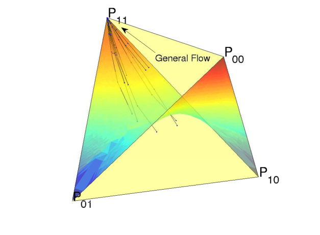
Figure 1: Geiringer manifold (colored) and some trajectories for some random initial populations. The system’s convergence to dominance of the optimal genotype is indicated by the arrow.

As far as the fitness landscape is concerned the general parametrized two-locus two allele landscape is

$$f=a+b_{1}x_{1}+b_{2}x_{2}+cx_{1}x_{2}$$ (20)

where $c$ is the measure of the additive epistasis between the two loci. We take the genotype $I=00$ as the wild type, the genotypes $I=01$ and $10$ as single mutants and $I=11$ as a double mutant which is the optimal genotype. There are just three main landscape categories for the two-bit, two-locus model:

1. The wild type and the double mutant are the anti-optimum and optimum respectively.

2. One of the single mutants (10 or 01) is the antioptimum.

3. The two lowest fitness phenotypes are the single mutants.

Any other case can be brought to one of the previous by a relabeling that doesn’t affect the dynamics. In the first two landscape types, a generic population will always eventually evolve towards the global optimum. In the third type, the population may converge to the optimum or the suboptimal wild type $00$ depending on the initial population and the recombination probability.

From Equations (10) and (13) we have

$$\Delta_{P_{ij}}(t)=\left(\frac{f_{ij}}{\bar{f}(t)}-1\right)-p_{c}\Delta_{ij}(t)$$ (21)

$$\Delta_{\bar{f}}(t)=\frac{\overline{f^{2}}_{s+r}(t-1)}{{\bar{f}}_{s+r}(t-1)}-\frac{\overline{f_{s}^{2}}(t-1)}{{\bar{f}}_{s}(t-1)}-p_{c}\sum_{ij}f_{ij}\Delta_{ij}(t)$$ (22)

For the optimal genotype

$$\Delta_{11}(t)=\frac{1}{{\bar{f}}^{2}(t)}(a(a+b_{1}+b_{2}+c)P_{11}(t)P_{00}(t)-(a+b_{1})(a+b_{2})P_{01}(t)P_{10}(t))$$ (23)

As mentioned, the sign of $\Delta_{ij}$ determines the qualitative effect of recombination in a given generation. To develop some intuition for how the characteristics of the landscape affect our metrics we will set for the moment $P_{ij}(t)=1/4$, i.e., a homogeneous population with no initial bias for one genotype versus another. As the parameter $a$ just sets the scale for the landscape we can without loss of generality for fitness proportional selection set $a=1$. We will also set $b_{1}=b_{2}=b$ so that both single mutants have the same fitness. In this case,

$$\Delta_{11}(t)=\frac{(c-b^{2})}{(1+b+c/4)^{2}}$$ (24)

For a multiplicative landscape $c=b^{2}$ and $\Delta_{11}=0$, as is well known. For an additive landscape $c=0$ and therefore $\Delta_{11}(t)=-b^{2}/(1+b)<0$. In this case recombination leads to a higher frequency of the optimal genotype in the next generation than selection alone. For a deceptive landscape, $b<0$, but $c>-2b$ and so $\Delta_{11}(t)>0$ and recombination in this region of the parameter space leads to a lower frequency of the optimal genotype in the next generation. In terms of BBs, for deceptive landscapes, the marginal fitnesses are such that $f_{1*}<f_{0*}$ and $f_{*1}<f_{*0}$, and so the reason why recombination is unfavourable is that the necessary mutant alleles for constructing the optimal genotype are deleterious relative to the corresponding alleles of the genotype $00$. For additive epistasis, such that $c>b^{2}$, we have $\Delta_{11}(t)>0$ and recombination once again leads to a lower frequency of the optimal genotype in the next generation than selection alone. Generally, if we take $c-b^{2}<0$ as signifying negative multiplicative epistasis then we see that in such landscapes recombination has a positive effect in terms of our $\Delta$ metric and on the contrary for positive multiplicative epistasis. Note that the additive limit $c=0$ corresponds to negative multiplicative epistasis. Interestingly, equation (24) shows that the greatest benefit from recombination, i.e., the minimum value of $\Delta_{11}$ is associated with landscapes with negative additive epistasis, i.e., $c<0$. Maximum negative epistasis is given by the minimum value of $c$, $c=-b$. In this case $\Delta_{11}(t)=-b(1+b)/(1+3b/4)^{2}$.

Why would this maximum negative epistasis be associated with the utility of recombination, at least in terms of metric (10)? Examining equation (23) we see that the first term, proportional to $P_{11}(t)P_{00}(t)$, corresponds to elimination of the optimal genotype $11$ by recombining it with the suboptimal genotype $00$, whereas the term proportional to $P_{01}(t)P_{10}(t)$ corresponds to construction of $11$ via recombination of the single mutants $10$ and $01$. It is the competition between these two effects that measures the benefits of recombination in terms of (10). Additive landscapes with $c=0$ reduce the impact of destruction without compromising the positive effect of reconstruction. Negative epistasis, on the other hand, does not affect the construction of the optimal genotype by recombining the single mutants, but it does minimize the effect of destruction of the optimal genotype. The maximal effect is when $c=-b$ and corresponds to a Boolean ”OR” landscape where $f_{01}=f_{10}=f_{11}>f_{00}$. This is the situation where there is genetic redundancy, as the fitness of the optimal phenotype requires the presence of only one optimal allele not both. At this naive level we also see that the benefit of recombination is not restricted to small negative multiplicative epistasis but, rather, the larger the additive negative epistasis the larger the benefit conferred by it.

In terms of the metric (11) the contribution from recombination is given by

$$\sum_{ij}f_{ij}\Delta_{ij}(t)=c\Delta_{11}(t)=\frac{c(c-b^{2})}{(1+b+c/4)^{2}}$$ (25)

For this term to give a positive contribution to the average population fitness we require $c(c-b^{2})<0$. For $c>0$ this requires $c<b^{2}$, which we will term weak positive additive epistasis. On the other hand, for $c<0$, $c(c-b^{2})>0$ and recombination apparently leads to a decrease in the average population fitness, while in the additive limit, $c=0$, there is no change. Together, a one generation analysis of our two metrics would indicate that there are benefits to recombination from both of them only for weakly positively additively epistatic landscapes such that $c>0$ and $c<b^{2}$. We will characterize these landscapes as being “modular”, i.e., quasi-additive. It is important however, to go beyond a single generation, and for that we will consider metric (13) in section 5.

4.1.1 Muller’s Ratchet.

Muller’s ratchet [5], and variations thereof, have been frequently invoked in considerations of the potential benefits of recombination. Essentially, the argument is that recombination increases the evolvability of a population by allowing beneficial mutations on different genomes to be recombined into one more efficiently than the process of generating a double mutation. Similarly, deleterious mutations can be eliminated more efficiently from a population by having them recombined into a single genome, thus allowing selection to eliminate them more efficiently. We will consider these arguments in the context of our two locus system.

There are two regimes of interest related to Muller’s ratchet, one is that advantageous mutations appear in a population and the second that deleterious mutations appear. The question is: How does recombination affect the dynamics of these mutants? Considering the first case, if we consider the population to be such that the fit double mutant is absent, i.e., $P_{11}(t)=0$, then $\Delta_{11}=(P^{\prime}_{11}(t)P^{\prime}_{00}(t)-P^{\prime}_{10}(t)P^{\prime}_{01}(t))=-P^{\prime}_{10}(t)P^{\prime}_{01}(t)<0$. So

$$\Delta_{P_{11}}(t)=\left(\frac{f_{11}}{\bar{f}(t)}-1\right)P_{11}(t)+p_{c}P^{\prime}_{10}(t)P^{\prime}_{01}(t)$$ (26)

$$\delta_{\bar{f}}(t)=(\bar{f^{2}}-{\bar{f}}^{2})+p_{c}(f_{11}-f_{01}-f_{10}+f_{00})P^{\prime}_{10}(t)P^{\prime}_{01}(t).$$ (27)

From Equation (26) we see that the number of fit double mutants increases from generation $t$ to generation $t+1$ due to the effect of recombination relative to selection only dynamics. This is, in fact, independent of the fitness landscape, being associated with the search regime of recombination alluded to in section 2.1. In contrast, in Equation (27), we see that the average population fitness will increase in the presence of recombination if and only if $F^{(2)}=(f_{11}-f_{01}-f_{10}+f_{00})>0$, which is a direct measure of the degree of additive epistasis between the two loci. As noted, for a purely additive landscape, $F^{(2)}=0$ and so recombination is neutral in this setting. For the other genotypes we have the fraction of wild types increases due to the effect of recombination, while the frequency of single mutants decreases. What happens in the case where $P_{11}(t)\neq 0$ will be considered in section 5 as the benefit from recombination then depends on the actual population as well as the landscape.

Turning now to the case of deleterious mutants: in this case we take the wild type to be the genotype $11$ and the types $01$ and $10$ to be deleterious single mutants and $00$ to be an even more deleterious double mutant. In this case, just as for beneficial mutants, $\Delta_{11}=(P^{\prime}_{11}(t)P^{\prime}_{00}(t)-P^{\prime}_{10}(t)P^{\prime}_{01}(t))=-P^{\prime}_{10}(t)P^{\prime}_{01}(t)<0$ and hence the proportion of optimal wild types $11$ increases. In terms of average population fitness, the increase from generation $t$ to $t+1$ is given by Equation (27). In other words the change in average population fitness per generation for the case of beneficial versus deleterious mutations is identical if we are considering the same fitness landscape.

4.1.2 Asymptotic behavior of $\Delta$

Before going on to consider the full numerical solution of the two-locus model we will consider what can be said analytically about the asymptotic behavior of the system. Although there are 7 parameters that control the dynamics, the asymptotic behavior can be most naturally written in terms of just two parameters

$$C(t)\equiv\frac{P_{11}P_{00}}{P_{10}P_{01}},$$ (28)

where, for brevity, we use $P_{ij}$ for $P_{ij}(t)$, and

$$A\equiv\frac{f_{10}f_{01}}{f_{11}f_{00}}.$$ (29)

The one generation evolution equation for $C(t)$ is

$$C(t+1) = \frac{P_{11}(t+1)P_{00}(t+1)}{P_{10}(t+1)P_{01}(t+1)}=\frac{(P^{\prime}_{11}-p_{c}\Delta)(P^{\prime}_{00}-p_{c}\Delta)}{(P^{\prime}_{10}+p_{c}\Delta)(P^{\prime}_{01}+p_{c}\Delta)}$$ (30)

$$= \frac{\frac{P^{\prime}_{11}P^{\prime}_{00}}{\Delta}-p_{c}(P^{\prime}_{11}+P^{\prime}_{00})+p_{c}^{2}\Delta}{\frac{P^{\prime}_{10}P^{\prime}_{01}}{\Delta}+p_{c}(P^{\prime}_{10}+P^{\prime}_{01})+p_{c}^{2}\Delta}$$

Without loss of generality we again choose $I=11$ to be the optimal genotype. The evolution of the genotype frequencies, $P_{ij}$, as given by equation (1), ensures the eventual dominance of one of the genotypes. The first part of this derivation is analogous to section 3 in [35]. We suppose a priori that the limit

$$C_{\infty}\equiv\lim_{t\rightarrow\infty}C(t)$$ (31)

exists, which in turn implies that

$$\lim_{t\rightarrow\infty}\frac{P^{\prime}_{11}P^{\prime}_{00}}{\Delta}=\frac{C_{\infty}}{C_{\infty}-A}$$ (32)

and

$$\lim_{t\rightarrow\infty}\frac{P^{\prime}_{10}P^{\prime}_{01}}{\Delta}=\frac{A}{C_{\infty}-A}$$ (33)

With these elements in hand we can calculate the putative limit of equation (30) to find:

$$C_{\infty}=\frac{\frac{C_{\infty}}{C_{\infty}-A}-p_{c}}{\frac{A}{C_{\infty}-A}},$$ (34)

Solving this last equation for $C_{\infty}$ we obtain:

$$C_{\infty}=\frac{p_{c}A}{p_{c}+A-1},$$ (35)

Finally, since $\Delta=P^{\prime}_{11}P^{\prime}_{00}-P^{\prime}_{10}P^{\prime}_{01}$ and $C^{\prime}=\frac{P^{\prime}_{11}P^{\prime}_{00}}{P^{\prime}_{10}P^{\prime}_{01}}$, we note that the negativity of $\Delta$ is equivalent to the condition

$$C^{\prime}_{\infty}\equiv\lim_{t\rightarrow\infty}\frac{P^{\prime}_{11}P^{\prime}_{00}}{P^{\prime}_{10}P^{\prime}_{01}}\equiv\frac{C_{\infty}}{A}=\frac{p_{c}}{p_{c}+A-1}<1,$$ (36)

which reduces to $A>1$ for $p_{c}\neq 0$. So, we can see that the asymptotic benefit of recombination in terms of increasing the fraction of optimal genotypes relative to selection only, is determined by only 2 parameters - $A$ and $p_{c}$ and is independent of the initial population.

With this formula in hand, we can easily map any fitness landscape to a range of values for $A$ and thus determine if recombination will be asymptotically favorable for that particular landscape. we have

$$A=\frac{(a+b_{1})(a+b_{2})}{a(a+b_{1}+b_{2}+c)},$$ (37)

To simplify further the visualization of the asymptotic behavior, we again assume that $b\equiv b_{1}=b_{2}$, i.e., that the two mutants have the same fitness. As eventually the optimal genotype dominates for non-deceptive landscapes, recombination is asymptotically neutral. However, how $\Delta$ approaches zero depends on $A$. Small values of values of $b$ and $c$ correspond to a more neutral fitness landscape, where selection effects are small. For an additive landscape $A>1$ and so recombination is asymptotically beneficial in that $\Delta$ tends to zero from negative values. Small values of $b$ relative to $c>0$ correspond to highly positively additively epistatic landscapes and in this case $A<1$ and recombination is asymptotically disadvantageous in that $\Delta$ approaches zero from positive values. The multiplicative landscape with $c=b^{2}$ and, hence, $A=1$, separates the two classes of behavior. The dependence of the parameter $A$ (=$\frac{f_{01}f_{10}}{f_{00}f_{11}})$ as a function of $b$ and $c$ is shown in the next graph: Values of $A$ greater than $1$ mean that the iterates must eventually reach negative values of $\Delta$. The sign of $\Delta$ is then conserved, although the magnitude approaches zero as the system reaches linkage equilibrium associated with a population dominated by the optimal genotype. The opposite happens when $A<1$. Note that the locus defined by the intersection of the surfaces $A(b,c)$ and $A=0$ is given by $b^{2}=c$ and corresponds to the case of multiplicative landscapes.

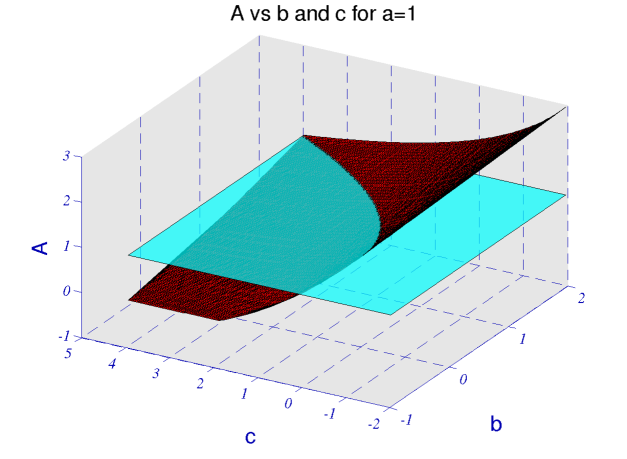
Figure 2: $A(b,c)=\frac{f_{01}f_{10}}{f_{00}f_{11}}$ for $a=1$. The solid plane, $A=1$, separates those fitness landscapes that according to Eq.36 will eventually benefit from recombination from those that don’t.

5 Exact Numerical Results

Turning now to the non-asymptotic behavior, we performed an exploration of the 7 dimensional parameter space of the two-locus, two-allele system to determine under which conditions recombination is beneficial in terms of our two metrics (21) and (22). In such a high dimensional space, visualization of the resulting graphs requires separation into several distinct cases. We set $p_{c}=0.5$ in all the following as $p_{c}$ just affects the magnitude of the effects of recombination but not whether it is beneficial or not as this is controlled by the sign of $\Delta$.

5.1 Recombination as a function of fitness landscape

We first consider graphs for arbitrary fitness landscapes but for a fixed initial population, with a further subdivision into cases made according to the type of initial population. As we have fixed $b_{1}=b_{2}=b$ and set $a=1$ we display the graphs as functions of $b$ and $c$. The valid region, all fitnesses positive with the genotype $11$ as optimum, is given by $b>-1$, $c>-2b$ and $c>-b$. The deceptive region is given by $b<0$. For ease of interpretation we also show lines associated with the multiplicative limit $b^{2}=c$ (yellow) and the additive limit $c=0$ (green). Note that both the additive and multiplicative limits require $b>0$. The “needle-in-a-haystack” landscape is given by $b=0$, $c>0$ and lies on the border that separates non-deceptive and deceptive landscapes. The point $b=0$, $c=0$ corresponds to a flat fitness landscape where there is no selection pressure.

Two kinds of graphs are provided, one that displays the value of the SWLD coefficient in different generations, and another that displays $\Delta_{\bar{f}}$ (Equation (13)), defined as the change in average fitness between generation $t$ and generation $t+1$ in a population evolving with both selection and recombination minus the change in average fitness of the same population but evolving with selection only. In the graphs we show four representative time slices - $t=1$, 2, 6, and 10 generations after the initial one. The plane $\Delta_{11}=0$ that separates the recombination advantageous/disadvantageous regimes is displayed (turquoise in the online version). For a given generation, those values of $b$ and $c$ where $\Delta_{11}<1$ are shaded in red (below the $\Delta_{11}=0$ plane), while those where $\Delta_{11}>1$ correspond to a darker shading (above the $\Delta_{11}=0$ plane).

5.1.1 Initial Population $P_{00}\approx 1$

In this first case we consider the dynamics when the initial population is dominated by the non-optimal wild type $00$, with $P_{00}(0)=0.8999$, $P_{01}(0)=0.05$, $P_{10}(0)=0.05$, $P_{11}(0)=0.0001$. So, we are here interested in the effects of recombination on the dynamics of favourable mutations as a function of the fitness landscape and in the background of an initial population dominated by a non-optimal wild type. We fix $a=1$ and study the variation in $\Delta$ as a function of $b$ and $c$, remembering the restrictions $2b+c>0$ and $b+c>0$. The most notable feature of 3 is that negative values of $\Delta$ are most associated with additive or negatively epistatic landscapes. Note that earlier in the evolution, $t=1$, the benefits of recombination are clear to see, even for quite positively epistatic interactions with only deceptive landscapes showing a disadvantage. This, however, is due to this region being still in the search regime, as the initial frequency of optimal genotypes was zero. Gradually, the population moves away from the search regime and enters the modular regime, where we see that it is only for landscapes that are either weakly positively epistatic, additive or negatively epistatic that recombination is beneficial. Note that the relative benefit of recombination is not fixed but evolves, thus showing the dependence on the relative frequencies of the different genotypes. In terms of BBs, $\Delta$ becomes positive when $P_{11}>P_{1*}P_{*1}$ so, as the frequency of the optimal type increases, eventually recombination becomes unfavourable relative to selection only, with the point at which it becomes unfavourable, $P_{11}=P_{1*}P_{*1}$, being dependent on the fitness landscape, as well as the initial population.

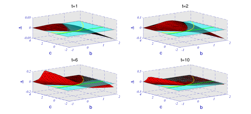
Figure 3: Value of $\Delta$ at different generations for two-locus two-allele system as a function of fitness landscape, characterized by $b$ and $c$. The initial population is $P_{00}(0)=0.8999$, $P_{01}(0)=0.05$, $P_{10}(0)=0.05$, $P_{11}(0)=0.0001$. The $\Delta=0$ plane has been marked to distinguish between conditions in which recombination is favorable ($\Delta<0$) or not. The curve on the plane is $c=b^{2}$, the condition for a multiplicative landscape.

Turning now to the graphs of the change in average fitness of the population; at $t=1$, in the search regime, we see that recombination leads to an increase in average population fitness, over and above that of selection only, for basically all landscapes. This is due to the addition of optimal genotypes in an initial population dominated by the non-optimal wild type. Gradually, however the effect of recombination diminishes as one enters the modular regime so that for positively epistatic landscapes the difference between selection only and recombinative dynamics is minimal. However, we note that there is still a strong pronounced effect for either weakly positively epistatic, additive or weakly negatively epistatic landscapes.

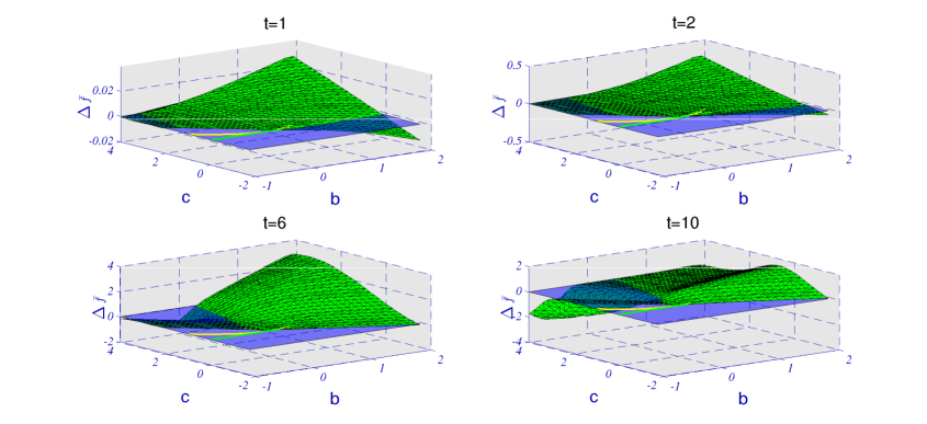
Figure 4: Value of $\Delta_{\bar{f}}$ at different generations for the two-locus two-allele system as a function of fitness landscape, characterized by $b$ and $c$. The initial population is $P_{00}(0)=0.8999$, $P_{01}(0)=0.05$, $P_{10}(0)=0.05$, $P_{11}(0)=0.0001$. The $\Delta_{\bar{f}}=0$ plane has been marked to distinguish between conditions in which recombination is favorable ($\Delta_{\bar{f}}>0$) or not.

So, how do we interpret these results in terms of BBs? Both in the search and modular regimes the advantage of recombination is associated with the fact that BBs of the optimal genotype, $1*$ and $*1$, are recombined to form the type $11$. As the graphs show, this recombination of BBs is, in fact, a more efficient process in generating optimal types and increasing overall population fitness than selection alone for weakly epistatic landscapes. In fact, the benefit in the search regime is actually relatively independent of the degree of epistasis of the landscape. Later on though, in the modular regime, the generation of optimal genotypes by recombining optimal BBs competes against the generation that evolved through pure selection effects. For positively epistatic landscapes, once there are enough optimal types selection can produce new ones as or more efficiently than recombination. For modular landscapes however, recombination retains its advantage. Indeed, this is, in fact, what characterizes the modular regime, i.e., that weakly epistatic BBs or modules are juxtaposed by recombination into even fitter genotypes leading to a faster evolution and a faster increase in average population fitness. The fact that the recombination is even more beneficial in the presence of additive negative epistasis is due to the fact that the destruction of the optimal type produces two single mutants that have fitness very similar to that of the optimal type. This is the advantage of genetic redundancy.

5.1.2 Initial Population $P_{11}\approx 1$

We now turn to the case where the initial population is dominated by the optimal genotype as the wild type with the presence of genotypes with a single deleterious mutation and a small proportion of deleterious double mutant genotypes. Specifically, $P_{11}(0)=0.8999$, $P_{10}(0)=0.05$, $P_{01}(0)=0.05$ and $P_{00}(0)=0.0001$. The question now is: What is the dynamics of the deleterious mutations in the population as a function of the landscape parameters? Once again, we fix $a=1$ and study the variation in $\Delta$ as a function of $b$ and $c$,

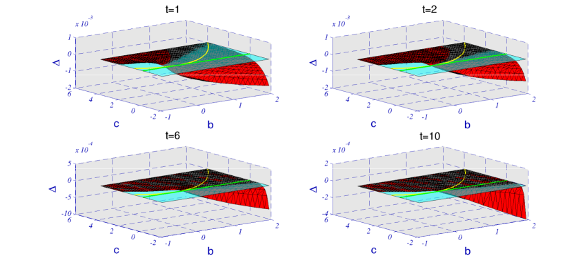
Figure 5: Value of $\Delta$ at different generations for two-locus two-allele system as a function of fitness landscape, characterized by $b$ and $c$. The initial population is $P_{11}(0)=0.8999$, $P_{10}(0)=0.05$, $P_{01}(0)=0.05$ and $P_{00}(0)=0.0001$. The $\Delta=0$ plane has been marked to distinguish between conditions in which recombination is favorable ($\Delta<0$) or not. The curve on the plane is $c=b^{2}$, the condition for a multiplicative landscape.

In Figure 5 the first thing to notice is that, in distinction to the case where the initial population is dominated by the non-optimal genotype, here there is no dinstinct behavior associated with the search regime, as the optimal genotype is already dominant in the population. Thus, for positively epistatic landscapes the difference due to recombination is small. However, for additive or negatively epistatic landscapes we see that recombination is advantageous, with the advantage being more significant in the presence of negative epistasis. This is due to the fact that in such landscapes the elimination of the suboptimal double mutant $00$ is more efficient.

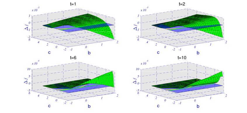
Figure 6: Value of $\Delta_{\bar{f}}$ at different generations for the two-locus two-allele system as a function of fitness landscape, characterized by $a$ and $c$. The initial population is $P_{11}(0)=0.8999$, $P_{10}(0)=0.05$, $P_{01}(0)=0.05$ and $P_{00}(0)=0.0001$. The $\Delta_{\bar{f}}=0$ plane has been marked to distinguish between conditions in which recombination is favorable ($\Delta_{\bar{f}}>0$) or not.

Considering now the average population fitness, we see clearly in Figure 6 how the advantage of recombination manifests itself in the modular regime where epistasis is weak. Interestingly, we see how negatively epistatic landscapes are, in the early part of the evolution, associated with $\Delta_{\bar{f}}<0$. This is due to the fact that for negative epistasis the overall contribution to the population fitness of a deleterious double mutant and an optimal genotype is less double mutant, selection can eliminate the mutations thereby purifying the population more efficiently than selection alone. The more modular the landscape the more efficient this process becomes.

5.1.3 Initial Population $P_{11}\approx 0$, $P_{00}\approx\frac{1}{2}$, $P_{01}\approx P_{10}\approx\frac{1}{4}$

We now consider a scenario similar to that of sub-section 5.1.1, where the initial proportion of optimal genotypes is zero; but now, however, the frequency of the BBs, $1*$ and $*1$, represented by the beneficial mutants $01$ and $10$, relative to the less fit wild type $00$ is much higher. Concretely, the initial population is: $P_{11}(0)=0.0001$, $P_{10}(0)=0.25$, $P_{01}(0)=0.25$ and $P_{00}(0)=0.4999$ so that the BBs $1*$ and $*1$ form about a quarter of the population each one.

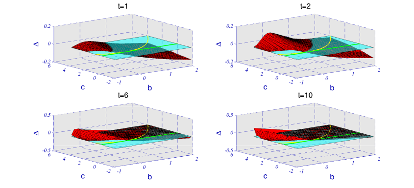
Figure 7: Value of $\Delta$ at different generations for two-locus two-allele system as a function of fitness landscape, characterized by $b$ and $c$. The initial population is $P_{00}(0)=0.4999$, $P_{01}(0)=0.25$, $P_{10}(0)=0.25$, $P_{11}(0)=0.0001$. The $\Delta=0$ plane has been marked to distinguish between conditions in which recombination is favorable ($\Delta<0$) or not. The curve on the plane is $c=b^{2}$, the condition for a multiplicative landscape.

We see in Figure 7 that the graphs are qualitatively similar to those of Figure 3. The chief difference now is that recombination is even more disadvantageous in the search regime for deceptive landscapes than before and more advantageous for modular landscapes - weak or zero positive epistasis or negative epistasis. This is due to the wider availability of the BBs $1*$ and $*1$ thus obstructing/facilitating the construction of the optimal type $11$ according to whether the landscape is deceptive or modular. As evolution progresses, as before, we see a passage from the search regime to the modular regime, where the relative benefit of recombination is restricted to weakly positively epistatic, additive or negatively epistatic landscapes.

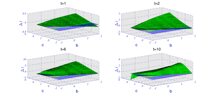
Figure 8: Value of $\Delta_{\bar{f}}$ at different generations for the two-locus two-allele system as a function of fitness landscape, characterized by $b$ and $c$. The initial population is $P_{11}(0)=0.0001$, $P_{10}(0)=0.25$, $P_{01}(0)=0.25$ and $P_{00}(0)=0.4999$. The $\Delta_{\bar{f}}=0$ plane has been marked to distinguish between conditions in which recombination is favorable ($\Delta_{\bar{f}}>0$) or not.

Similarly, in Figure 8 we see a similarity with the corresponding graphs of Figure 4 the average population fitness showing a strong increase, relative to the selection only case, due to the efficient formation of the optimal type, which in its turn is due to the large number of BBs in the population. Even for strongly epistatic landscapes there is a strong benefit to recombination in this regime. At later times, in the modular regime, we see that the advantage of recombination is again associated with additive, weakly positively epistatic or negatively epistatic landscapes, i.e., modular landscapes.

So, we see that the principle effect of increasing the BB frequency in the initial population is to accelerate the rate of evolution so that the frequency of the optimal genotype and the average population fitness increase more rapidly.

5.1.4 Initial Population $P_{11}\approx 0$, $P_{00}\approx 0$

We now look at an even more extreme case, where the initial population is completely dominated by the single mutants $01$ and $10$ with the initial population being $P_{11}(0)=0.0001$, $P_{10}(0)=0.4999$, $P_{01}(0)=0.4999$ and $P_{00}(0)=0.0001$. Qualitatively the results are as in sub-sections 5.1.3 and 5.1.1; the strong presence of the BBss $1*$ and $*1$ leading to a very efficient production of the optimal genotype $11$. This is, in fact, another good illustration of Muller’s ratchet. Although recombination leads to the generation of optimal genotypes it also leads to the production of the sub-optimal double mutants $00$. The latter, however, as the graphs clearly show, are flushed out by selection. In fact, as Figure 9 shows, they are produced and then flushed out most efficiently in the presence of recombination for modular landscapes when compared to selection only.

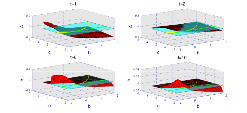
Figure 9: Value of $\Delta$ at different generations for two-locus two-allele system as a function of fitness landscape, characterized by $b$ and $c$. The initial population is $P_{11}(0)=0.0001$, $P_{10}(0)=0.4999$, $P_{01}(0)=0.4999$ and $P_{00}(0)=0.0001$. The $\Delta=0$ plane has been marked to distinguish between conditions in which recombination is favorable ($\Delta<0$) or not. The curve on the plane is $c=b^{2}$, the condition for a multiplicative landscape.

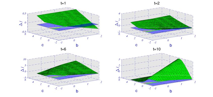
Figure 10: Value of $\Delta_{\bar{f}}$ at different generations for the two-locus two-allele system as a function of fitness landscape, characterized by $b$ and $c$. The initial population is $P_{11}(0)=0.0001$, $P_{10}(0)=0.4999$, $P_{01}(0)=0.4999$ and $P_{00}(0)=0.0001$. The $\Delta_{\bar{f}}=0$ plane has been marked to distinguish between conditions in which recombination is favorable ($\Delta_{\bar{f}}>0$) or not.

5.1.5 Initial Homogeneous Population $P_{ij}=0.25$

The final initial population type we will consider is that of a uniform initial population where all genotypes have the same initial frequency, $0.25$. Here we see behaviour that is qualitatively similar to that found for other populations. The chief difference here is that given the ample presence of the optimal genotype in the initial population there is no search regime and so the dynamics begins and remains in the modular regime. With no population bias we can see the role played by the multiplicative limit with at $t=1$ $\Delta$ being positive for landscapes with positive multiplicative epistasis and, particularly, deceptive landscapes. It is negative for weakly postively epistatic, additive and negatively epistatic landscapes. As evolution progresses we can see that the relative advantage diminshes such that at $t=10$ the advantage of recombination is only noticeable for larger negative epistasis.

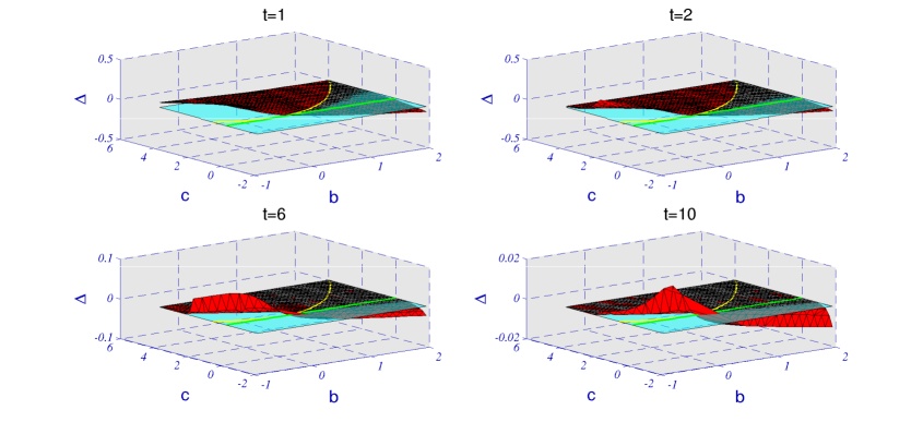
Figure 11: Value of $\Delta$ at different generations for two-locus two-allele system as a function of fitness landscape, characterized by $b$ and $c$. The initial population is $P_{ij}(0)=0.25$. The $\Delta=0$ plane has been marked to distinguish between conditions in which recombination is favorable ($\Delta<0$) or not. The curve on the plane is $c=b^{2}$, the condition for a multiplicative landscape.

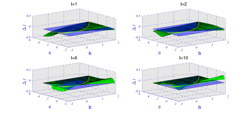
Figure 12: Value of $\Delta_{\bar{f}}$ at different generations for the two-locus two-allele system as a function of fitness landscape, characterized by $b$ and $c$. The initial population is $P_{ij}(0)=0.25$. The $\Delta_{\bar{f}}=0$ plane has been marked to distinguish between conditions in which recombination is favorable ($\Delta_{\bar{f}}>0$) or not.

In terms of average population fitness in Figure 12 we see an analogous story: at $t=1$ average population fitness is increased only for landscapes with negative multiplicative epistasis, up to the additive limit, but is, in fact, negative for negative additive epistasis. However, as evolution progresses, once again, we see the dominant role played by modular landscapes - i.e., weakly positively epistatic, additive and negatively epistatic landscapes.

5.2 Recombination as a function of population

Having explored the effect of recombination on the space of fitness landscapes, by varying continuously the landscape parameters $b$ and $c$ for a variety of distinct initial populations, we now consider the complementary viewpoint of considering how the effect of recombination changes by varying continuously the initial population for a variety of fixed fitness landscapes. Due to the conservation of probability, the population vector is characterized by only three frequencies. For simplicity of visualization we will consider intitial populations such that $P_{01}(0)=P_{10}(0)$ and consider the population dynamics as a function of $P_{11}(0)$ and $P_{01}(0)$.

A general observation on almost all the graphs in this section is that since there is generic convergence to the optimal genotype $P_{11}=1$ for non-deceptive landscapes so clearly all the surfaces have $\Delta=0$ in the $P_{11}=1$ corner.

5.2.1 Additive landscape $a=1,b_{1}=b_{2}=1,c=0$.

The first landscape we will consider is an additive landscape ($c=0$). For this landscape (Figure 13) the tendency is clear, that the more BBs and the fewer optimal types there are, the more recombination helps. This is again a manifestion of the search regime. In this landscape, as can be seen at $t=1$, recombination in terms of $\Delta$ is only unfavorable when the proportion of optimal types is appropriately larger than the frequencies of the BBs, as then selection can act more efficiently to increase the frequency of the optimal type than can recombination of the single mutants. However, we see that this effect is temporary. By $t=6$ basically any initial population is associated with $\Delta<0$. We can see that the SWLD increases in time, approaching zero asymptotically, this regime being associated with the approach to a population completely dominated by the optimal genotype. This dynamics, in fact, shows an important universality associated with recombination, that demonstrates the role of Muller’s ratchet: that the action of recombination is to drive the system to particular frequencies for the optimal type and its BBs that correspond to quite special initial conditions at $t=0$. To understand this, note that at $t=6$ and $t=10$ the proportion of optimal types is high. If we imagine the value of $P_{11}(t=6)$, for example, that is a consequence of evolution in the presence of recombination, then we can map those values such as to imagine them as initial conditions, say at $t=1$, for further evolution. However, we can observe at $t=1$ that values of $P_{11}$ close to 1 correspond to positive values of $\Delta$ except in a very narrow wedge where the values of $P_{01}$ are as high as possible. This wedge is associated precisely with a lower relative frequency of the suboptimal $00$ genotype. The conclusion is that recombination is removing the suboptimal $00$ genotype more efficiently than selection only.

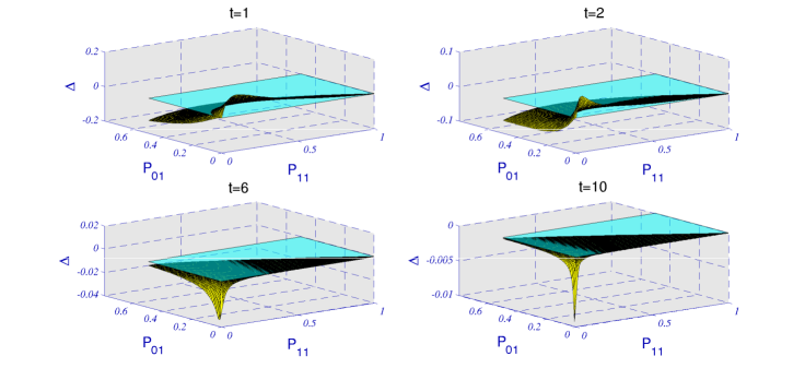
Figure 13: Value of $\Delta$ at different time steps for a two-locus two-allele system with an additive fitness landscape $a=1,b_{1}=b_{2}=1,c=0$) for different values of the initial population given by $P_{11}$ and $P_{10}(=P_{01})$. The $\Delta=0$ plane has been marked to distinguish between conditions in which recombination is favorable ($\Delta<0$) or not.

Finally, the presence of a trough associated with quite negative values of $\Delta$ for $t=6$ and $t=10$ is a consequence of th fact that the search regime is more extensive when the frequency of both optimal genotype and BBs is low.

5.2.2 Neutral landscape: $b_{1}=b_{2}=c=0$, $a\neq 0$ ($A=1$)

For a neutral landscape, where the effects of selection are null, as with the additive landscape, the “the more BBs the better recombination is” rule is valid, but we see a different behavior as a function of initial population. For neutral evolution, the SWLD, $\Delta$, and the standard linkage disequilibrium coefficient, $D$, are the same. So, Figure 14 shows the approach to the Geiringer or Robbins manifold, defined by $D=0$. The approach to this manifold is from the negative or positive side depending on whether the initial population is dominated by the BBs $01$ and $10$, or by the optimal genotype $11$. The Geiringer limit has been amply studied in the literature [27]. Thus, recombination is beneficial when there is an ample supply of BBs and few optimal types, and deleterious when there are no BBs. The minimal value of $\Delta$ is for $P_{01}(0)=0.5$ and the maximal for $P_{01}(0)=0$, $P_{00}(0)=P_{11}(0)=0.5$.

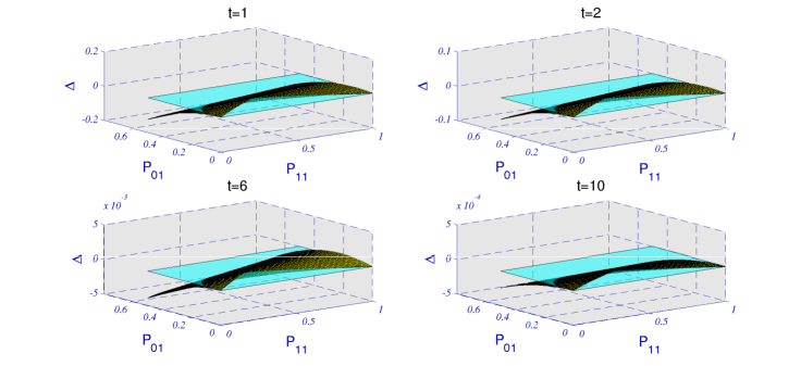
Figure 14: Value of $\Delta$ at different time steps for a two-locus two-allele system with a neutral ($b_{1}=b_{2}=c=0$, $a\neq 0$) fitness landscape for different values of the initial population given by $P_{11}(0)$ and $P_{10}(0)=P_{01}(0)$. The $\Delta=0$ plane has been marked to distinguish between conditions in which recombination is favorable ($\Delta<0$) or not.

5.2.3 Multiplicative landscape $a=1$, $b_{1}=b_{2}=2$, $c=4$

This landscape satisfies the multiplicative constraint that $ac=b^{2}$. Here we see that recombination is favorable in the search regime where the BB frequency is high and the frequency of the optimal genotype is low. However, for other than very small $P_{11}$ we can see that recombination is somewhat unfavorable when the BB frequency is relatively low but, in the main, it is generally neutral in its effects. This is consistent with known results for multiplicative landscapes. In fact, viewing the time evolution, even if one starts in the search regime we see that very quickly the system approaches linkage equilibrium.

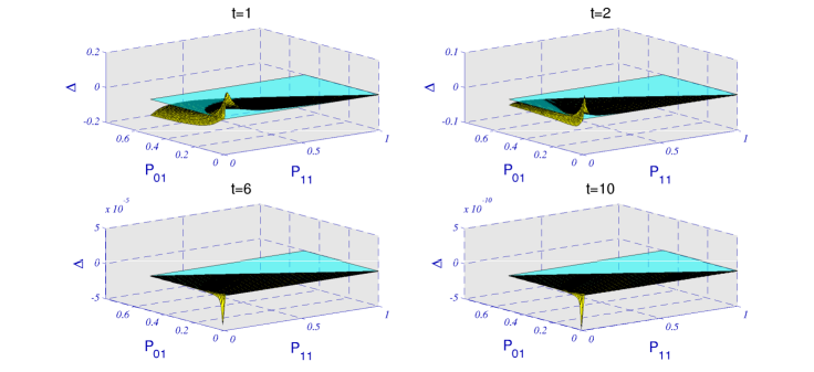
Figure 15: Value of $\Delta$ at different time steps for a two-locus two-allele system with a multiplicative fitness landscape ($a=1$, $b_{1}=b_{2}=2$, $c=4$) for different values of the initial population given by $P_{11}$ and $P_{10}(=P_{01})$. The $\Delta=0$ plane has been marked to distinguish between conditions in which recombination is favorable ($\Delta<0$) or not.

5.2.4 Needle-In-A-Haystack, $b_{1}=b_{2}=0$, $c\neq 0$, $a\neq 0$ ($A=\frac{a}{a+c}$)

We now turn to the case of a landscape with maximally positive epistasis - NIAH, which, as mentioned, has been used extensively in models of molecular evolution and, especially, in considerations of selection-mutation balance and the existence of error thresholds. Here, it corresponds to a Boolean “AND” function on the two loci. As a function of the initial population we can clearly see that in the search regime, where there is an ample supply of BBs and only a zero or small proportion of the optimal genotype, that recombination is favorable, both in terms of leading to a more efficient production of the optimal genotype when compared to selection only ($\Delta<0$) as well as a more fit population ($\Delta_{\bar{f}}>0$, Figure 17). On the other hand, away from the search regime it is clear that the effects of recombination are unfavorable. Note that the advantage or disadvantage of recombination decreases in time as the system gets closer to linkage equilibrium, this equilibrium being associated with a population dominated by the optimal genotype.

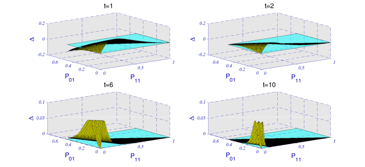
Figure 16: Value of $\Delta$ at different generations for a two-locus two-allele system with a “Needle in a haystack” fitness landscape ($b_{1}=b_{2}=0$, $c=0.001$, $a=1$) for different values of the initial population given by $P_{11}$ and $P_{10}(=P_{01})$. The $\Delta=0$ plane has been marked to distinguish between conditions in which recombination is favorable ($\Delta<0$) or not.

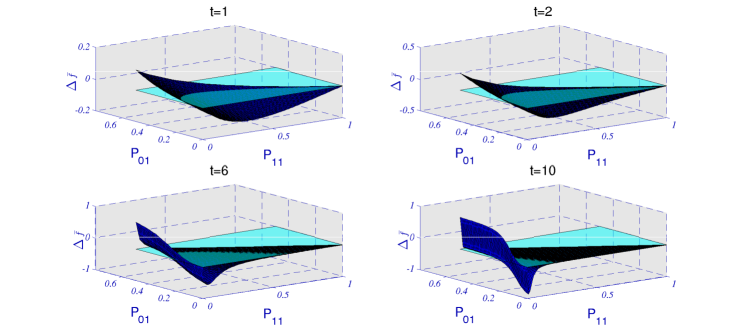
Figure 17: Value of $\Delta_{\bar{f}}$ at different generations for a two-locus two-allele system with a “Needle in a haystack” fitness landscape ($b_{1}=b_{2}=0$, $c=0.001$, $a=1$) for different values of the initial population given by $P_{11}$ and $P_{10}(=P_{01})$. The $\Delta_{\bar{f}}=0$ plane has been marked to distinguish between conditions in which recombination is favorable ($\Delta_{\bar{f}}>0$) or not.

5.2.5 Landscape with Genetic Redundancy, $a=1$, $b=1$, $c=-1$

For a landscape with maximal negative epistasis, corresponding to an ”OR” Boolean function on the two loci we see in Figure 18 that very rapidly recombination becomes beneficial in terms of $\Delta$ for any initial population.

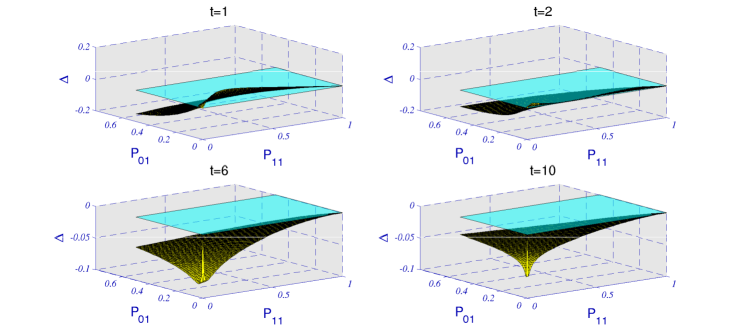
Figure 18: Value of $\Delta$ at different generations for a two-locus two-allele system with a fitness landscape with genetic redundancy ($b_{1}=b_{2}=1$, $c=-1$, $a=1$) for different values of the initial population given by $P_{11}$ and $P_{10}(=P_{01})$. The $\Delta=0$ plane has been marked to distinguish between conditions in which recombination is favorable ($\Delta<0$) or not.

5.2.6 Deceptive Landscape, $a=1$, $b=-0.5$, $c=2$

Finally, a deceptive landscape (Figure 19) offers a complete contrast to that of a redundant one, with recombination being disadvantageous in terms of $\Delta$ for any initial population.

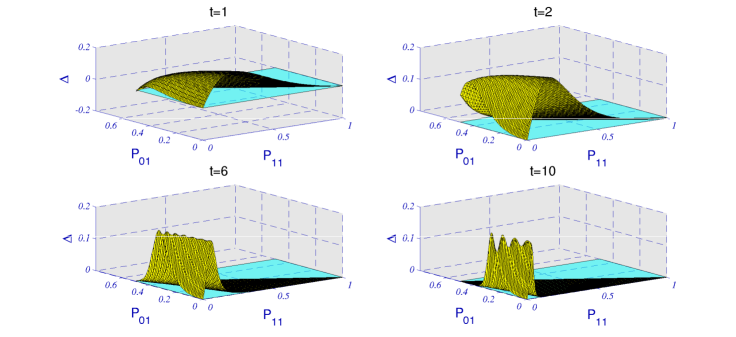
Figure 19: Value of $\Delta$ at different generations for a two-locus two-allele system with a deceptive fitness landscape ($b_{1}=b_{2}=-0.5$, $c=2$, $a=1$) for different values of the initial population given by $P_{11}$ and $P_{10}(=P_{01})$. The $\Delta=0$ plane has been marked to distinguish between conditions in which recombination is favorable ($\Delta<0$) or not.

6 Conclusion

As discussed in the introduction, genetic recombination remains a puzzle as far as having a full, intuitive understanding of why it is so prevalent, with no generally accepted explanation of its benefits. Many theoretical analyses have been performed. The vast majority of these have been in the context of variations on a theme of standard population genetics models - haploid, diploid, with modifer genes, without modifier genes, with finite population, with infinite population, with mutation, without mutation, with few loci, with many loci, with different fitness landscapes, with different population states etc. Of course, to understand the benefits of recombination in the context of a mathematical model, the model itself must contain a description of the mechanisms that explain why it is useful in the first place. The question is then: do the benefits lie outside the context of the models that have been studied, or are they hidden within the results of these models? If the former is true, then one must formulate a new model, with new features, which will then make manifest its utility. On the other hand, if the latter is the case, then it is important to have a model that can be studied exhaustively, in that there is no region of the parameter space of the model that remains unexplored. Additionally, the model should be such that the effective degrees of freedom of the underlying system are manifest.

Previous work [38, 39], both analytical and numerical, has hinted at the fact that recombination seems to be especially useful in the context of quasi-additive landscapes, while other work has shown a role for weak negative multiplicative epistasis. However, these analyses did not cover the full parameter space of the considered models, and so there is always doubt that the landscapes or initial populations considered were not representative and therefore any identified benefits of recombination were not “universal” but, rather, tied to the specific scenario considered. To counter these arguments, in this paper, we have taken the route of fixing a simple model - a two locus, two allele system of haploid sequences with non-overlapping generations evolving in the presence of selection and homologous recombination - but have analyzed the full parameter space of the model. This corresponds to three population variables and three landscape parameters. Having fixed the model, we can begin to look for the regions of parameter space, if any, in which recombination is beneficial. Of course, we first have to define what we mean by “beneficial”. In this paper we fixed two metrics: one was the SWLD coefficient for the optimal genotype that measures the excess production of such types over and above that which is produced by selection only; and the other is the increase in average population fitness over and above that which would be produced by selection only. With these two metrics we measure the benefits of recombination in terms of its capacity to lead to higher proportions of fitter genotypes and fitter populations relative to selection only.

So, what does our analysis of the parameter space of this model tell us? The analyses we have carried out are consistent with the previous results of [39] where it was shown that there are two important, but distinct, regimes in which recombination is beneficial in terms of both the metrics that we have used to characterize its benefits. The first of these is the search regime, which is associated with conditions where the fittest genotype is either not present or only at low frequency. In this regime the benefit from recombination is relatively independent of the fitness landscape. However, exactly how beneficial it is does depend on both the landscape and the actual population. The second regime we have termed the modular regime and is associated with weakly additively epistatic landscapes, i.e., quasi-additive landscapes. However, the fact that we have analyzed the set of possible landscapes and populations, allows us to go beyond this restricted analysis and observe and characterize several important universal properties of recombination.

Firstly, in terms of $\Delta$ there is a clear association between the sign of the epistasis and the sign of $\Delta$. Production of the optimal genotype ($11$) is more favorable in the presence of negative additive epistasis ($c<0$) than for positive additive epistasis ($c>0$) for beneficial mutations. It is also disfavored when single mutants ($01$ and $10$) are less fit ($b<0$) than the suboptimal genotype $00$. What is more, by following the dynamics across multiple generations, we see that recombinative evolution itself is directed towards favoring landscapes that are more and more modular, more and more negatively epistatic. This is a universal feature that is independent of the initial population.

In terms of the increase in average population fitness relative to selection only dynamics we see a profoundly interesting dynamic. For the different initial populations considered when investigating evolution as a function of landscape, we see that there is an initial regime (t=1) wherein there is a perceived benefit from recombination for a wide array of landscapes with, in fact, under some circumstances, a relative advantage for landscapes with positive versus negative additive epistasis. However, as evolution progresses, $t=10$, the benefit from recombination has become restricted to quasi-additive or negatively additively epistatic landscapes independently of the initial population. This is best understood by viewing Figure 12, where the initial population is homogeneous, which means that it begins on the Geiringer manifold. There, we see that recombination is disfavored initially ($t=1$) for any positively multiplicatively epistatic landscape - including deceptive landscapes - and for any additively negatively epistatic landscape. However, very quickly the universal tendency towards favoring quasi-additive and negatively additively epistatic landscapes sets in. There are many works [44, 45, 46], some recent [47, 48], in which the role of negative epistasis between mutations in evolution is discussed. It must be noted that in these references negative epistasis means sub-multiplicative epistasis, that is, epistasis is quantified with a parameter whose magnitude measures deviations of the logarithm of fitness from linearity as a function of the number of mutations. In our results we included both supra and sub-additive (concerning the sign of $c$) and supra and sub-multiplicative (concerning the sign of $ac-b^{2}$) epistatic regimes and, importantly it is the existence of negative additive epistasis that seems to be important for recombination.

As a function of the initial population, we see a complementary but completely consistent point of view relative to that of landscape. At $t=1$ we can see the effect of any initial linkage disequilibrium with the sign of $\Delta$ being strongly affected by the sign of $D$: more/less BBs relative to $11$ or $00$ being associated with $D<0$/$D>0$. The effect of deception is to disfavor recombination for basically any population, while for a genetically redundant landscape it is to favor it for any initial population.

We believe that the results of this paper unite various important threads of modern evolutionary thought - the ubiquity of genetic recombination, the ubiquity of modularity and, relatedly, the ubiquity of genetic redundancy, and thereby offer a quite universal explanation of why recombination is so widespread. This paper is not the appropriate forum in which to discuss the reasons why modularity and redundancy themselves are so important. There are many papers on the subject. However, it is amazing that the benefits of recombination seem to be so intimately tied to these phenomenon, at least in the framework of the fitness landscape paradigm as discussed here. In the space of all possible landscapes we have shown that the benefits of recombination are manifest only for quasi-additive or negatively additively epistatic landscapes, a quite restricted subset of landscape space. However, it is precisely such landscapes that seem to be so common in biology. In other words our conclusion is that recombination is so widespread because it leads to important evolutionary benefits only for systems that are modular and/or redundant and and it is precisely such landscapes that seem to be the norm. This leads, indeed, to another evolutionary “chicken and egg” puzzle. Did recombination evolve to take advantage of the existence of modularity and redundancy or vice versa? We would posit that there has been a strong co-evolutionary link between the them since the beginnings of life with recombination distributions and fitness landscapes co-evolving to maximize the benefits of one with the other.

So, what are weak points of our model and analysis? Well, first of all one could criticize the simplicity of the model, although the model shares many features with previous analyses. The fact that only two loci are considered is the price we pay for being able to consider the full parameter space. However, its worth mentioning again that these “loci” could represent different levels of description from, in principle, nucleotides up to entire sets of genes. Our other restriction is that we can describe each locus in terms of two possible states. We are quite sure that no qualitative effect that we have observed here depends on the existence of only two alleles. The question is: are the effects we see and the conclusions we make from the two locus model generalizable to multi-loci models? Unfortunately, we cannot analyze exhaustively the full parameter space of such a model. For $\ell$ loci there are, in principle, $2^{\ell}-1$ population parameters and $2^{\ell}$ landscape parameters to contend with.

However, there are some related analyses with multiple loci [49], investigating numerically the dynamics for certain specific landscapes and initial populations. The results seen there are completely consistent with what we observe in full generality in this paper, i.e., that the benefits of recombination when not in the search regime are manifest in modular landscapes while, on the contrary, it is detrimental in the presence of high positive epistasis. In this paper we have also neglected the effects of mutation, whereas much previous work has been associated with studying how recombination interacts with mutation by positing Muller’s ratchet type regimes where the dynamics of beneficial or detrimental single mutations are considered in the presence of recombination. It is an important question to understand the relative benefits of mutation versus recombination in the context of the metrics that we have considered here. We will, indeed, return to that in a separate paper. However, it is first important to understand what benefits there are that are intrinsic to recombination without a comparison with mutation.

Finally, we have also restricted attention here to fixed-length sequences. We believe that the relation between recombination and modularity extends beyond this restriction, applying also to variable-length sequences and recombination-like genetic operators other than homologous recombination. For instance, unequal crossing over or gene duplication.

7 Acknowledgements

This work was partially supported by DGAPA grant IN120509 and by a special Conacyt grant to the Centro de Ciencias de la Complejidad. DAR is grateful to the IIMAS, UNAM for use of their facilities. We are grateful to León Martínez and Michael Gaunt for discussions.

References

- [1] J. Maynard Smith, What use is sex?, Journal of Theoretical Biology 30 (2) (1971) 319–335.
- [2] I. Eshel, M. Feldman, et al., On the evolutionary effect of recombination, Theoretical population biology 1 (1) (1970) 88–100.
- [3] R. Fisher, The genetical theory of natural selection., Clarendon Press, 1930.
- [4] A. Kondrashov, Deleterious mutations and the evolution of sexual reproduction, Nature 336 (6198) (1988) 435–440.
- [5] H. Muller, Some genetic aspects of sex, The American Naturalist 66 (703) (1932) 118–138.
- [6] J. Felsenstein, The evolutionary advantage of recombination, Genetics 78 (2) (1974) 737.
- [7] N. Barton, B. Charlesworth, Why sex and recombination?, Science 281 (5385) (1998) 1986.
- [8] R. Watson, D. Weinreich, J. Wakeley, Genome structure and the benefit of sex, Wiley Online Library, 2011.
- [9] R. Kouyos, O. Silander, S. Bonhoeffer, Epistasis between deleterious mutations and the evolution of recombination, Trends in ecology & evolution 22 (6) (2007) 308–315.
- [10] P. Keightley, S. Otto, Interference among deleterious mutations favours sex and recombination in finite populations, Nature 443 (7107) (2006) 89–92.
- [11] S. Otto, T. Lenormand, et al., Resolving the paradox of sex and recombination, Nature Reviews Genetics 3 (4) (2002) 252–261.
- [12] B. Baker, A. Carpenter, M. Esposito, R. Esposito, L. Sandler, The genetic control of meiosis, Annual review of genetics 10 (1) (1976) 53–134.
- [13] M. Feldman, Selection for linkage modification: I. random mating populations, Theoretical Population Biology 3 (3) (1972) 324–346.
- [14] S. Otto, M. Feldman, Deleterious mutations, variable epistatic interactions, and the evolution of recombination, Theoretical population biology 51 (2) (1997) 134–147.
- [15] N. Barton, et al., A general model for the evolution of recombination, Genetical Research 65 (2) (1995) 123–144.
- [16] U. Liberman, M. Feldman, On the evolution of epistasis iii: the haploid case with mutation, Theoretical population biology 73 (2) (2008) 307–316.
- [17] L. Zhivotovsky, M. Feldman, F. Christiansen, Evolution of recombination among multiple selected loci: A generalized reduction principle, Proceedings of the National Academy of Sciences 91 (3) (1994) 1079.
- [18] B. Charlesworth, Mutation-selection balance and the evolutionary advantage of sex and recombination, Genet. Res 55 (3) (1990) 199–221.
- [19] J. Pepper, The evolution of modularity in genome architecture, Proceedings of the Artificial Life 7 (2000) 9–12.
- [20] F. Christiansen, S. Otto, A. Bergman, M. Feldman, Waiting with and without recombination: the time to production of a double mutant, Theoretical population biology 53 (3) (1998) 199–215.
- [21] W. Rice, et al., Experimental tests of the adaptive significance of sexual recombination, Nature Reviews Genetics 3 (4) (2002) 241–251.
- [22] C. R. Stephens, H. Waelbroeck, Schemata evolution and building blocks, Evol. Comp. 7 (1999) 109–124.
- [23] C. R. Stephens, The renormalization group and the dynamics of genetic systems, Acta Phys. Slov. 52 (2002) 515–524.
- [24] T. Nagylaki, J. Hofbauer, P. Brunovskỳ, Convergence of multilocus systems under weak epistasis or weak selection, Journal of mathematical biology 38 (2) (1999) 103–133.
-
[25]
R. Bürger, The
mathematical theory of selection, recombination, and mutation, Wiley series
in mathematical and computational biology, John Wiley, 2000.
URL http://books.google.com.mx/books?id=9oHwAAAAMAAJ - [26] P. Stadler, C. Stephens, Landscapes and effective fitness, Comments® on Theoretical Biology 8 (4-5) (2003) 389–431.
- [27] H. Geiringer, On the probability theory of linkage in mendelian heredity, The Annals of Mathematical Statistics 15 (1) (1944) 25–57.
- [28] L. Altenberg, The schema theorem and price’s theorem, Foundations of genetic algorithms 3 (1995) 23–49.
- [29] C. Stephens, H. Waelbroeck, Effective degrees of freedom in genetic algorithms, Physical Review E 57 (3) (1998) 3251.
- [30] R. Poli, J. Rowe, C. Stephens, A. Wright, Allele diffusion in linear genetic programming and variable-length genetic algorithms with subtree crossover, Genetic Programming (2002) 11–21.
- [31] D. E. Goldberg, Genetic algorithms and Walsh functions: Part I. A gentle introduction, Complex Systems 3 (1989) 123–152.
- [32] M. D. Vose, A. H. Wright, The simple genetic algorithm and the Walsh transform: Part II, the inverse, Evolutionary Computation 6(3) (1998) 275–289.
- [33] E. D. Weinberger, Fourier and Taylor series on fitness landscapes, Biological Cybernetics 65 (1991) 321–330.
- [34] A. H. Wright, The exact schema theorem, http://www.cs.umt.edu/CS/FAC/WRIGHT/papers/schema.pdf (January 2000).
- [35] M. Feldman, J. Crow, et al., On quasilinkage equilibrium and the fundamental theorem of natural selection., Theoretical Population Biology 1 (1970) 371–391.
- [36] A. Kondrashov, Deleterious mutations as an evolutionary factor: 1. the advantage of recombination, Genetical research 44 (02) (1984) 199–217.
- [37] B. Charlesworth, M. Morgan, D. Charlesworth, The effect of deleterious mutations on neutral molecular variation, Genetics 134 (4) (1993) 1289–1303.
- [38] C. Stephens, J. Cervantes, Just what are building blocks?, Foundations of Genetic Algorithms (2007) 15–34.
- [39] C. Stephens, E. Arenas, J. Cervantes, B. Peralta, E. Ricalde, C. Segura, When are building blocks useful?, in: Artificial Intelligence, 2006. MICAI’06. Fifth Mexican International Conference on, IEEE, 2006, pp. 217–228.
- [40] M. Eigen, Selforganization of matter and the evolution of biological macromolecules, Die Naturwissenschaften 10 (1971) 465–523.
- [41] C. Stephens, R. Poli, Coarse-grained dynamics for generalized recombination, Evolutionary Computation, IEEE Transactions on 11 (4) (2007) 541–557.
- [42] Y. Takahashi, Convergence of simple genetic algorithms for the two-bit problem., Bio Systems 46 (3) (1998) 235.
- [43] S. Karlin, et al., General two-locus selection models: some objectives, results and interpretations., Theoretical Population Biology 7 (3) (1975) 364.
- [44] R. Azevedo, R. Lohaus, S. Srinivasan, K. Dang, C. Burch, Sexual reproduction selects for robustness and negative epistasis in artificial gene networks, Nature 440 (7080) (2006) 87–90.
- [45] C. Burch, L. Chao, Epistasis and its relationship to canalization in the rna virus 6, Genetics 167 (2) (2004) 559–567.
- [46] T. MacCarthy, A. Bergman, Coevolution of robustness, epistasis, and recombination favors asexual reproduction, Proceedings of the National Academy of Sciences 104 (31) (2007) 12801–12806.
- [47] A. Khan, D. Dinh, D. Schneider, R. Lenski, T. Cooper, Negative epistasis between beneficial mutations in an evolving bacterial population, Science 332 (6034) (2011) 1193–1196.
- [48] S. Kryazhimskiy, J. Draghi, J. Plotkin, In evolution, the sum is less than its parts, science 332 (6034) (2011) 1160–1161.
- [49] D. Rosenblueth, C. Stephens, An analysis of recombination in some simple landscapes, MICAI 2009: Advances in Artificial Intelligence (2009) 716–727.