Periodic dynamics of fermionic superfluids in the bcs regime

Abstract

We study the zero temperature non-equilibrium dynamics of a fermionic superfluid in the BCS limit and in the presence of a drive leading to a time dependent chemical potential $\mu(t)$. We choose a periodic driving protocol characterized by a frequency $\omega$ and compute the fermion density, the wavefunction overlap, and the residual energy of the system at the end of $N$ periods of the drive. We demonstrate that the BCS self-consistency condition is crucial in shaping the long-time behaviour of the fermions subjected to the drive and provide an analytical understanding of the behaviour of the fermion density $n_{{\mathbf{k}}_{F}}$ (where ${\mathbf{k}}_{F}$ is the Fermi momentum vector) after a drive period and for large $\omega$. We also show that the momentum distribution of the excitations generated due to such a drive bears the signature of the pairing symmetry and can be used, for example, to distinguish between s- and d-wave superfluids. We propose experiments to test our theory.

1 Introduction:

Ultracold atoms provide us with a useful test bed for studying equilibrium and non-equilibrium properties of interacting many-body systems. The initial focus in these systems has been largely on bosonic atoms; in particular, the realization and the study of properties of Bose-Einstein condensates (BECs) has been the prime subject of investigation in the first few years of experimental studies on such systems [1]. In contrast, studies of fermionic atoms have gained momentum much later [2, 3]. The main experimental obstacle in studying many-body effects in fermionic atoms has been the realization of sufficiently low temperature so as to obtain a gas of quantum degenerate fermions with $T\leq T_{F}\sim\hbar^{2}n_{0}^{2/3}/(k_{B}m)$, where $m$ is the mass of the atoms and $n_{0}$ is their density, $T_{F}$ is the Fermi temperature of the gas and $k_{B}$ is the Boltzmann constant. However, recent experiments have made significant progress in this direction and it has been possible to observe the crossover from classical to quantum behaviour in fermionic gases [4]. The formation of Fermi superfluids, which is an interesting many-body phenomenon in its own right [5], required lower temperature and stronger interactions. It was soon realized that the latter can be achieved by utilizing the Feshbach resonance phenomenon which allows for tuning of both the strength and the sign of the interaction between the fermions. A major hindrance in realizing such strong interactions for bosonic atoms has been three-body losses; in contrast, such losses are minimal for fermionic atoms due to the Pauli exclusion principle. This allows for the possibility of stable fermionic condensates with strong inter-particle interaction which acts as a test bed for studying Fermi superfluids and, in particular, the BCS-BEC crossover in these systems. Several recent experiments have verified this phenomenon by numerous measurements in both the BCS and the BEC side of the crossover [6].

The dynamical properties of Fermi superfluids have also received theoretical and experimental attention in the recent past. On the experimental side, there have been several studies such as probing the expansion of Fermi superfluids after a sudden release of the trap potential [7], measurement of collective excitations of these superfluids [8], measurement of the superfluid gap by radio-frequency (RF) spectroscopy [9], and observation of vortex dynamics [10]. On the theoretical side, several studies were made to study the equilibrium and near-equilibrium properties of these systems. In particular, early studies concentrated on understanding the crossover phenomenon by approaching it from the BCS side [11]. These have been later supplemented by inclusion of more sophisticated diagrammatic techniques over the BCS mean-field theory [12], study of the effect of presence of a trap potential [13], inclusion of bosonic molecular degree of freedom in the BCS Hamiltonian [14], and use of quantum Monte Carlo methods [15]. Later works focused on non-equilibrium aspects of these systems based on hydrodynamic approach for studying low-lying collective excitations [16], vortex dynamics [17], quench dynamics across a BCS-BEC crossover [18], and properties of dynamic structure factors of these superfluids in the weak-interaction regime [19].

Non-equilibrium dynamics of closed quantum systems have recently received a lot of theoretical attention due to the possibility of realizing such dynamics in ultracold atom systems [20, 21, 22, 23, 24, 25, 26, 27, 28, 29, 30, 31, 32]. Most of such studies in this direction have concentrated on bosonic or spin Hamiltonians realized by bosonic ultracold atoms in optical lattices [27, 29, 30, 31]. In particular, experimental realizations of Ising-like spin model [33] and Bose-Hubbard model [34] have provided impetus to such theoretical studies. More recently, concrete experiments were carried out on the dynamics of bosons near the superfluid-insulator transition [35]. The results of such experiments are in qualitative agreement with theoretical studies on such systems [31]. Similar attempts of experimental realization of the Ising model have recently been undertaken in trapped ion systems [36, 37]. However, such studies have not been carried out extensively on fermionic atoms in the superfluid state.

In this work, we study the response of a fermionic superfluid in the BCS regime to a periodic drive. We choose a specific driving protocol which leads to a time-dependent periodic chemical potential for the fermions characterized by a frequency $\omega$: $\mu(t)=\mu_{0}+\mu_{a}\sin(\omega t)$. We note that such periodic drives are known to lead to a host of interesting phenomena in quantum systems. For example, it has been observed that coherent periodic driving in a class of integrable quantum many-body systems can give rise to novel quantum phenomena like dynamical many-body freezing, where non-monotonic freezing behaviour (with respect to the driving frequency) is observed [28]. A variant of this phenomenon has also been predicted for ultracold bosons in optical lattices [38]. The aim of the present work is to study the effect of such a drive on superfluid fermions.

The key results that we obtain from such a study are the following. First, we show that the BCS self-consistency condition plays a crucial role in shaping the response of such superfluids to the periodic drive and hence establish that the dynamics of fermionic superfluids will be fundamentally different from those of integrable systems such as Ising or Kitaev models which can be described by Bogoliubov-like Hamiltonians without the self-consistency condition. We demonstrate this by computing the fermion density (which can be easily related to the magnetization of the Ising and Kitaev models) which displays oscillatory behaviour as a function of time for the Ising system and approaches a constant at long time for the self-consistent BCS system. We also derive an analytical formula for the $\omega$ dependence of the fermion density $n_{{\mathbf{k}}_{F}}$ (or equivalently magnetization $m_{{\mathbf{k}}_{F}}$) at the gap edge (where ${\mathbf{k}}_{F}$ is the Fermi momentum vector) after a complete drive cycle and in the limit of large drive frequency. Second, we compute the wavefunction overlap (and hence the defect density) and the residual energy of the systems after single and multiple cycles of the drive and discuss the dependence of these quantities on $\omega$. Finally, we compute the momentum distribution of the excitations created due to the drive at the end of one drive cycle and show that such a distribution depends on the pairing symmetry of the fermionic superfluid. Thus we demonstrate that the dynamic response of these superfluid may prove to be a useful tool for determining its pairing symmetry.

The plan of the rest of paper is as follows. In section 2, we introduce the model and the corresponding BCS mean-field equations and provide explicit expressions for the observables that we shall compute. In section 3, we present numerical results for several observables such as the defect density, its momentum distribution, and the residual energy at the end of a drive cycle and discuss their properties. This is followed by an analytical treatment of the self-consistent problem in section 4 where we obtain an analytical expression for the $\omega$ dependence of $m_{{\mathbf{k}}_{F}}$ at high $\omega$. We provide a discussion of our work and suggest possible experiments to test our theory in section 5 and provide some calculational details in the appendix.

2 Formalism

In this section, we introduce the formalism and define the main physical observables which we shall compute numerically. The Hamiltonian for a gas of interacting ultracold fermions in a shallow square optical lattice at $T=0$, in the absence of any drive, is given by

$$H(t) = \sum_{{\mathbf{k}}\sigma}\left[\epsilon_{\bf k}-\mu_{0}\right]\hat{c}^{\dagger}_{{\mathbf{k}}\sigma}\hat{c}_{{\mathbf{k}}\sigma}$$ (1)

$$-g\sum_{{\mathbf{k}},{\mathbf{k}^{\prime}},{\mathbf{k}^{\prime\prime}}}\hat{c}^{\dagger}_{{\mathbf{k}}+{\bf k^{\prime\prime}}\uparrow}\hat{c}^{\dagger}_{{\mathbf{k}^{\prime}}-{\mathbf{k}^{\prime\prime}}\downarrow}\hat{c}_{{\bf k^{\prime}}\downarrow}\hat{c}_{{\mathbf{k}}\uparrow}.$$

Here $\hat{c}_{{\mathbf{k}}\sigma}$ represent the annihilation operators for fermions of momentum ${\mathbf{k}}$ and spin $\sigma=\{\uparrow,\downarrow\}$. The first term represents the kinetic energy of the fermions, and the second term the four-fermion interaction energy with amplitude $g>0$ which represents attractive interaction between the fermions. Here $\epsilon_{\mathbf{k}}=-2J\sum_{i}\cos(k_{i})$ is the band energy spectrum for the fermions, the index $i$ takes values $x$ and $y$ for $d=2$ or $x$, $y$, and $z$ for $d=3$, and $\mu_{0}$ is the chemical potential. In the rest of this work, we shall assume that the trap potential is slowly-varying so that a locally constant chemical potential $\mu_{0}=\epsilon_{F}$ (where $\epsilon_{F}$ is the Fermi energy viz. the energy at  the Fermi momentum vector ${\mathbf{k}}_{F}$) can be used to describe the fermions in the trap. In the BCS regime and at zero temperature, the ground state of the fermions is a superfluid whose excitations can be described by the BdG equations

$$E({\mathbf{k}})\left(\begin{array}[]{c}u_{\mathbf{k}}\\ v_{\mathbf{k}}\end{array}\right) = \left(\begin{array}[]{cc}(\epsilon_{\mathbf{k}}-\mu_{0})&\Delta({\mathbf{k}})\\ \Delta^{\ast}({\mathbf{k}})&-(\epsilon_{\mathbf{k}}-\mu_{0})\end{array}\right)\left(\begin{array}[]{c}u_{\mathbf{k}}\\ v_{\mathbf{k}}\end{array}\right),$$ (8)

where $u_{\mathbf{k}}$ and $v_{\mathbf{k}}$ are the amplitudes of the particle and the hole in a BdG quasiparticle and are related to the BCS wavefuntion by

$$|\psi\rangle = \prod_{\mathbf{k}}(u_{\mathbf{k}}+v_{\mathbf{k}}\hat{c}_{\bf k}^{\dagger}\hat{c}_{{\bf-k}}^{\dagger})|0\rangle.$$ (10)

The pair-potential $\Delta({\mathbf{k}})$ depends on the pairing symmetry and is given by

$$\Delta({\mathbf{k}}) = \Delta_{0},\quad{\rm s-wave},$$

$$\Delta({\mathbf{k}}) = \Delta_{0}[\cos(k_{x})-\cos(k_{y})],\quad{\rm d}_{x^{2}-y^{2}}{\rm-wave}.$$ (11)

In the rest of this work, we shall mostly consider s-wave pairing except while discussing momentum distribution of the defect density in section 3, where we shall discuss other pairing symmetries. Our analysis, which will be detailed in this section, can be easily generalized to other pairing symmetries. For the rest of this work, we set $\hbar=1$.

For s-wave pairing, the pair potential satisfies the self-consistency relation

$$\Delta_{0} = g\sum_{\mathbf{k}}u_{\mathbf{k}}^{\ast}v_{\mathbf{k}}.$$ (12)

Equation (LABEL:bdg1) and (12) admit the well-known BCS solution

$$E({\mathbf{k}}) = \pm\sqrt{(\epsilon_{{\mathbf{k}}}-\mu_{0})^{2}+|\Delta_{0}|^{2}},$$

$$u^{\rm eq}_{\mathbf{k}} = \frac{1}{\sqrt{2}}\left[1+\frac{(\epsilon_{\mathbf{k}}-\mu_{0})}{E({\mathbf{k}})}\right]^{1/2},$$

$$v^{\rm eq}_{\mathbf{k}} = \frac{1}{\sqrt{2}}\left[1-\frac{(\epsilon_{\mathbf{k}}-\mu_{0})}{E({\mathbf{k}})}\right]^{1/2}e^{-i\phi_{0}}.$$ (13)

Here, $\phi_{0}$ is the phase of $\Delta_{0}$. We now introduce a time-dependent drive, $\mu(t)=\mu_{0}+\mu_{a}\sin(\omega t)$, so that $\mu_{a},\,\omega\ll J$. This can be achieved in typical experimental systems by introducing an additional time-dependent harmonic trap potential which is sufficiently broad so as to allow for a uniform fermion density. In this regime, the response of the system to the drive can be described by the time-dependent Bogoliubov de-Gennes equation given by

$$i\partial_{t}\left(\begin{array}[]{c}u_{\mathbf{k}}(t)\\ v_{\mathbf{k}}(t)\end{array}\right) = \left(\begin{array}[]{cc}(\epsilon_{\mathbf{k}}-\mu(t))&\Delta({\bf k;t})\\ \Delta^{\ast}({\mathbf{k}};t)&-(\epsilon_{\mathbf{k}}-\mu(t))\end{array}\right)$$ (21)

$$\times\left(\begin{array}[]{c}u_{\mathbf{k}}(t)\\ v_{\mathbf{k}}(t)\end{array}\right),$$

together with the self-consistency condition which, for s-wave pairing, reads

$$\Delta({\mathbf{k}};t) \equiv \Delta(t)=g\sum_{\mathbf{k}}u^{\ast}_{\bf k}(t)v_{\mathbf{k}}(t).$$ (22)

In the rest of this work, we consider the system to be in the superfluid ground state at $t=t_{i}$ with $(u_{\mathbf{k}}(t_{i}),v_{\bf k}(t_{i}))=(u^{\rm eq}_{\mathbf{k}},v_{\mathbf{k}}^{\rm eq})$ and study its evolution in the presence of the periodic drive till a time $t_{f}$ which correspond to $N$ cycles of the drive $t_{f}=NT=2\pi N/\omega$, where $N$ is an integer.

In order to study such dynamics, we focus on the following key observables. First, we define the wavefunction of the BCS system $|\psi(t)\rangle=\prod_{\mathbf{k}}|\psi_{\mathbf{k}}(t)\rangle$, where we have denoted

$$|\psi(t)\rangle = \prod_{\mathbf{k}}\left(u_{\mathbf{k}}(t)+v_{\mathbf{k}}(t)\hat{c}_{\mathbf{k}}^{\dagger}\hat{c}_{{\bf-k}}^{\dagger}\right)|0\rangle,$$ (23)

with $u_{\mathbf{k}}(t)$ and $v_{\mathbf{k}}(t)$ being solutions of  (21) and (22). We now compute the effective magnetization $m(t)$, defined as

$$m_{\mathbf{k}}(t) = \langle\psi_{\mathbf{k}}(t)|\tau_{z}|\psi_{\mathbf{k}}(t)\rangle,$$

$$m(t) = \sum_{\mathbf{k}}m_{\mathbf{k}}(t)=\sum_{\mathbf{k}}[1-2|v_{\bf k}(t)|^{2}],$$ (24)

where $\tau_{z}$ is the Pauli matrix in particle-hole space. The observable $m(t)$ shall be equal to $m(t_{i})$ after a full drive cycle at $T=2\pi/\omega$ both in the impulse (where the wavefunction does not have time to adjust to the drive) and adiabatic limit (where the system remains in the ground state of the instantaneous Hamiltonian). Note that $m(t)$ is the magnetization of the Ising or Kitaev models described by BdG-like equations in their fermionic representations sans the self-consistency condition [25, 28]. For BCS fermions, $m(t)$ can be easily related to the time-dependent fermion density $n(t)$ using the relation

$$n(t) = \sum_{{\mathbf{k}}}\langle\psi_{\bf k}(t)|\left(\sum_{\sigma}\hat{c}^{\dagger}_{\bf k\sigma}\hat{c}_{\bf k\sigma}\right)|\psi_{\bf k}(t)\rangle=2\sum_{\mathbf{k}}|v_{\mathbf{k}}(t)|^{2}=1-m(t),$$ (25)

Thus $m(t)$ proves to be useful in comparing the behaviour of integrable Ising and Kitaev models with that of the non-integrable self-consistent BCS model. To this end, we also define the long time average of $m(t)$

$$Q\equiv\lim\limits_{n\to\infty}\frac{1}{nT}\int^{nT}_{0}{\mathrm{d}}t\times m(t),$$ (26)

which shall also be used for such comparisons.

The second quantity which we compute is the wavefunction overlap. To compute this, we first define the amplitudes $u_{\mathbf{k}}^{\rm ad}(t)$ and $v_{\mathbf{k}}^{\rm ad}(t)$ which correspond to the values of $u_{\mathbf{k}}$ and $v_{\mathbf{k}}$ at time $t$ for adiabatic evolution. The amplitude $u_{\mathbf{k}}^{\rm ad}(t)$ is always real in our choice of gauge. The ground state of $H$ with $\mu=\mu(t)$ can be written in terms of these quantities as

$$|\psi^{\rm ad}(t)\rangle = \prod_{\mathbf{k}}\left(u_{\mathbf{k}}^{\rm ad}(t)+v_{\mathbf{k}}^{\rm ad}(t)\hat{c}_{\mathbf{k}}^{\dagger}\hat{c}_{{\bf-k}}^{\dagger}\right)|0\rangle,$$

$$u^{\rm ad}_{\mathbf{k}}(t) = \frac{1}{\sqrt{2}}\bigg{\{}1+\frac{\left[\epsilon_{\mathbf{k}}-\mu(t)\right]}{E({\mathbf{k}};t)}\bigg{\}}^{1/2},$$

$$v^{\rm ad}_{\mathbf{k}}(t) = \frac{1}{\sqrt{2}}\bigg{\{}1-\frac{\left[\epsilon_{\mathbf{k}}-\mu(t)\right]}{E({\mathbf{k}};t)}\bigg{\}}^{1/2}e^{-i\phi_{0}(t)}.$$ (27)

where $E({\mathbf{k}};t)=\sqrt{[\epsilon_{\mathbf{k}}-\mu(t)]^{2}+|\Delta(t)|^{2}}$, and $|\psi^{\rm ad}(t)\rangle$ is the adiabatic ground state continued in time. Also, $\phi_{0}(t)$ is the phase of $\Delta(t)$. Note that $|\psi^{\rm ad}(t_{f})\rangle=|\psi^{\rm ad}(t_{i})\rangle$ at the end of any integer number of drive cycles. We now define the wavefunction overlap $F$ as

$$F = |\langle\psi^{\rm ad}(t)|\psi(t)\rangle|^{2}$$ (28)

$$= \prod_{\mathbf{k}}F_{\mathbf{k}}=\prod_{\mathbf{k}}|u^{\rm ad}_{\bf k}(t)u_{\mathbf{k}}(t)+v^{\rm ad}_{\mathbf{k}}(t)v_{\mathbf{k}}(t)|^{2}.$$

The defect density or the density of excitations generated due the dynamics at any instant of time can be written in terms of $F$ as

$$\rho_{d} = \sum_{\mathbf{k}}\rho_{d}({\mathbf{k}})$$ (29)

$$\rho_{d}({\mathbf{k}}) = 1-F_{\mathbf{k}}=|u^{\rm ad}_{\mathbf{k}}(t)v_{\mathbf{k}}(t)-v^{\rm ad}_{\mathbf{k}}(t)u_{\mathbf{k}}(t)|^{2}.$$

Note that the defect density identically vanishes for adiabatic dynamics and thus provides a suitable measure for deviation from adiabaticity.

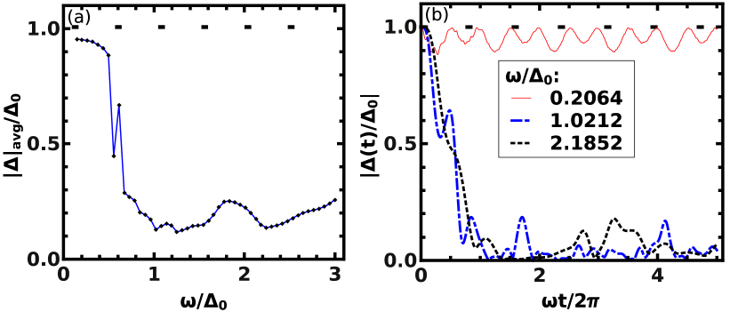
Figure 1: (Colour online) Plots of the long time average and instantaneous values of the amplitude of the order parameter $\Delta(t)$. The left panel shows the plot of the long time averaged $|\Delta(t)|$ (averaged over $10$ cycles of the drive) with respect to the drive frequency $\omega$. The right panel shows variation of the instantaneous values of $|\Delta(t)|$ with time $t$ (in units of $2\pi/\omega$) for several representative values of $\omega$ indicated in the legend. In both panels, $\Delta_{0}$ is indicated by a black dashed horizontal line.

Finally, we shall compute the residual energy which is the additional energy put in the system due to the drive. This is defined as the difference between the energy of the system at time $t$ and the adiabatic ground state energy and can be written as

$$E_{r}(t) = \sum_{\bf k}\left[\langle\psi_{\mathbf{k}}(t)|h_{\bf k}(t)|\psi_{\mathbf{k}}(t)\rangle\right.$$ (30)

$$\left.-\langle\psi_{\mathbf{k}}^{\rm ad}(t)|h_{\mathbf{k}}(t)|\psi_{\mathbf{k}}^{\rm ad}(t)\rangle\right]$$

$$= \frac{1}{g}\left[\Delta^{2}(t)+\Delta^{\ast 2}(t)-2\Delta^{2}_{0}\right]$$

$$-\sum_{\mathbf{k}}\left[\epsilon_{\mathbf{k}}-\mu(t)\right][m_{\bf k}(t)-m^{\rm ad}_{\mathbf{k}}(t)],$$

where $m_{\mathbf{k}}^{\rm ad}=1-2|v^{\rm ad}_{\mathbf{k}}|^{2}$. Note that the residual energy also vanishes for adiabatic dynamics.

Before closing this section, we note that the BCS self-consistency condition imparts dynamics to the order parameter $\Delta$ which can be written, using  (21) and (22), as

$$\dot{\Delta}(t) = ig\Big{\{}\Delta^{\ast}(t)m(t)+2\sum_{\mathbf{k}}\left[\epsilon_{\mathbf{k}}-\mu(t)\right]u^{\ast}_{\mathbf{k}}(t)v_{\mathbf{k}}(t)\Big{\}}.$$

If the time dependence of $\Delta$ is ignored or rendered negligible, then the system reverts to an ensemble of decoupled two-level systems in momentum space with constant gap $\Delta_{0}$. In this case, the dynamics is described by Landau-Zener-Stückelberg theory [39]. As we shall see in the next section, we reach this regime for $\omega/\Delta_{0}\ll 1$; however, the behaviour of a BCS system differs significantly from that of a bunch of decoupled two-level system for moderate $\omega$ for which $\omega/\Delta_{0}\sim 1$.

3 Numerical results

In this section, we discuss the self-consistent numerical evaluation of  (21) and (22) for $d=2$ and subsequent computations of $m(t)$, $Q$, $|\Delta(t)|$, $\rho_{d}$, and $E_{r}$ as defined in section 2. We have solved  (21) and (22) for BCS fermions in a $144\times 144$ square optical lattice and having unit hopping amplitude ($J=1$). The equilibrium gap and chemical potential has been taken to be $\Delta_{0}=0.1$ and $\mu_{0}=0.01$ respectively. The periodic drive term has been taken to be of the form $\mu_{a}\sin(\omega t)$ with $\mu_{a}=0.1$.

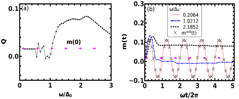
Figure 2: (Colour online) Left Panel: Plot of $Q$ as a function of $\omega$ with averaging carried over $10$ drive cycles. Right panel: Plot of $m(t)$ as a function of $\omega t/2\pi$ for representative values of $\omega$ indicated in the legend. A few representative values of the adiabatic magnetization $m^{adb}(t)$ is shown using crosses. In both panels, the initial values of $Q$ and $m$ is indicated by a magenta dashed horizontal line and all parameters are same as in figure 1.

We first consider the plot of the gap amplitude $|\Delta|$ in figure 1. The left panel of figure 1 shows the average gap amplitude as a function of the drive frequency $\omega$ after an average over $10$ cycles. We find that the average value of the gap amplitude decreases rapidly with increasing frequency and keeps fluctuating about $|\Delta|\simeq 0.2\Delta_{0}$ for large $\omega/\Delta_{0}\geq 2$. The right panel shows a plot of $|\Delta(t)|/\Delta_{0}$ as a function of $\omega t/2\pi$. We find that at small $\omega\ll\Delta_{0}$, $|\Delta(t)|$ displays oscillatory behaviour with maximum and minimal values of $\Delta_{0}$ and $0.9\Delta_{0}$ respectively. However, for $\omega\geq\Delta_{0}$, the behaviour of $|\Delta(t)|$ is qualitatively different; it decreases rapidly to near-zero values within the first couple of drive cycles ($\omega t/2\pi\leq 2$) and continues to fluctuate around this value for longer drive times, never returning close to its original value $\Delta(0)$. We note that such a behaviour of $|\Delta(t)|$ clearly reflects the importance of the self-consistency condition in the dynamics; any analysis with $|\Delta(t)|\simeq\Delta_{0}$ at all times is expected to produce qualitatively wrong results for $\omega\geq\Delta_{0}$.

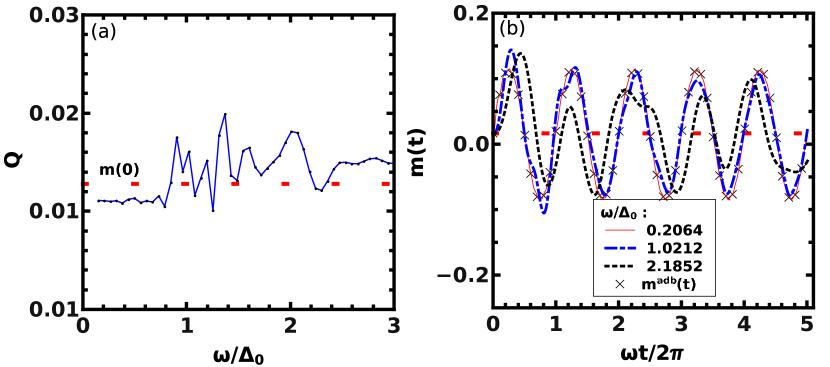
Figure 3: (Colour online) Same as in  figure 2 but for the non-self-consistent dynamics.

Next, we plot the effective magnetization $m(t)$ as a function of time $t$ and its time average $Q$ as a function of the drive frequency $\omega$. For the self-consistent dynamics appropriate for fermions in the BCS regime, as shown in  figure 2, there are clearly three regimes, one crossing over to the other as $\omega$ is increased. For $\omega\ll\Delta_{0}$, $m(t)$ (right panel) oscillates with large amplitude, following the drive almost adiabatically, resulting in $Q=m(0)$. The oscillations, though large, respects the symmetry of the drive, i.e., the long time average of the magnetization vanishes with the DC part of the drive, viz. the equilibrium chemical potential $\mu_{0}$. As $\omega$ approaches $\Delta_{0}$, this symmetry is destroyed, resulting $Q\neq m(0)$. For $\omega>\Delta_{0}$, the oscillatory behaviour of $m(t)$ with large amplitude is replaced by relaxation to an approximately constant value (with negligible fluctuations) within few initial cycles (right panel). This constant value determines the value of $Q$ (left panel), and we find that it deviates steadily from $m_{0}$ as $\omega$ is increased for $\omega<2.5\Delta_{0}$. We note that for $\omega>\Delta_{0}$, the mixing of the ${\mathbf{k}}$ modes of the quasiparticle excitations, which originates from the presence of the self-consistency condition and is therefore absent in Ising or Kitaev systems, is at the heart of such a deviation. Any hysteresis or freezing of the magnetization that would cause the drive symmetry to break was observed in periodically driven transverse Ising chains for large amplitudes and frequencies [28], and is also seen here for the self-consistent case at $\omega\lesssim\Delta_{0}$. For very large $\omega$, we of course see the behaviour of $m(t)$ crossing over to a regime where $Q\rightarrow m(0)$ again – here $\omega$ becomes too large for the system to react at all, and $m(t)$ remains frozen around $m(0)$ for all time (the regime sets in beyond $\omega>2.4\mbox{ }\Delta_{0}$).

The above behaviour is to be contrasted with the non-self-consistent case summarized in figure 3. Here $m(t)$ always executes a large, almost synchronized oscillation, approximately following the adiabatic path (black crosses in the right panel of figure 3). Naturally, the resulting values of $Q$ are close to $m(0)$ (albeit with some small fluctuations). This suggests that the synchronous oscillation is simply a manifestation of the near-adiabatic nature of the dynamics. Synchronization could also occur due to self dephasing of the system, after all the transients (some of them having power-law tails) have died down, due to quantum interference between the modes [28, 40]. But such synchronization would appear only in the $\omega t\rightarrow\infty$ limit, unlike in the present case, where the effect is visible from the very first cycle. The qualitative departure from this behaviour in the self-consistent case seems to stem from the non-adiabaticity induced by the self-consistency condition (22) which makes the effective Hamiltonian non-linear. The overlapping eigenfunctions of the non-linear Hamiltonian makes the criteria for adiabatic behaviour much more restricted compared to a linear case (see. e.g., Yukalov [41]). We shall address the behaviour of $m_{{\mathbf{k}}_{F}}(t)$ in a more quantitative manner in section 4, where we shall show that the value of $m_{{\mathbf{k}}_{F}}$ after one drive cycle decays as $1/\omega$ for $\omega\gg\Delta_{0}$.

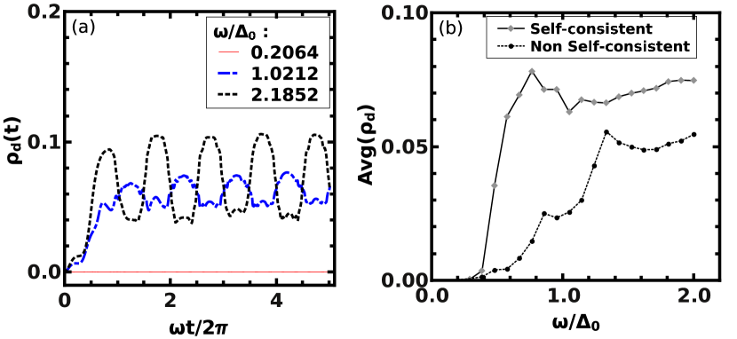
Figure 4: (Colour online) Left panel: Plot of the instantaneous defect density $\rho_{d}(t)$ as a function of $\omega t/(2\pi)$. The values of the drive frequency $\omega$ is indicated in the inset. Right panel: Plots of the long time average (averaged over $10$ drive cycles) of the defect density (both the non-self-consistent and the self-consistent cases) as a function of the drive frequency $\omega$.

Next, we consider the behaviour of the defect density $\rho_{d}$ as shown in figure 4. Here, as expected, the defect density becomes significant only for $\omega\geq\Delta_{0}$. The plot of the self-consistent defect dynamics shown in the left panel of figure 4 demonstrates that the defect density is an oscillatory function of $\omega$. The time-averaged defect density shown in the right panel of figure 4 for both the non-self-consistent and the self-consistent dynamics shows that these quantities display qualitatively similar behaviour. A similar behaviour is seen for the residual energies as can be seen from figure 5. We find that $E_{r}(t)$ vanishes for $\omega\ll\Delta_{0}$ and displays oscillatory behaviour for $\omega\geq\Delta_{0}$. The behaviour of residual energy and the defect density clearly shows that the system wavefunction never comes back to itself for any $\omega$; thus BCS superfluids do not seem to support dynamic freezing as predicted for superfluid bosons by Mondal, Pekker and Sengupta  [38].

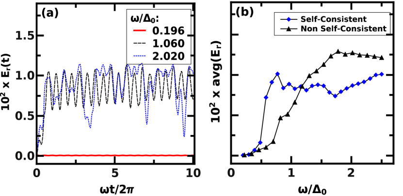
Figure 5: (Colour online) Same as in figure 4 but for residual energy $E_{r}$.

Finally, we consider the momentum distribution of the defect density at the end of a drive cycle and compare such plots for d-wave and s-wave pairing symmetries. The generalization of our calculation for d-wave pairing symmetry is straightforward and constitutes changing $\Delta_{0}\to\Delta_{\mathbf{k}}=\Delta_{0}[\cos(k_{x})-\cos(k_{y})]$ in  (21) and (22). The rest of the computation follows exactly as charted out in section 2. We expect the momentum distribution of the defect density to be qualitatively different for s- and d-wave pairing symmetries. For s-wave, the defect density has a uniform pattern in the Brillouin zone as expected from the momentum independence of the order parameter. In contrast, for the d-wave pairing symmetry, $\Delta({\mathbf{k}})$ vanishes at $k_{x}=\pm k_{y}$. It is easy to see from  (21) that for such momenta, one has

$$u_{\mathbf{k}}(t) = \theta(-f_{\mathbf{k}})e^{-i\int^{t}_{t_{i}}[\epsilon_{\mathbf{k}}-\mu(t^{\prime})]dt^{\prime}},$$

$$v_{\mathbf{k}}(t) = \theta(f_{\mathbf{k}})e^{i\int^{t}_{t_{i}}[\epsilon_{\mathbf{k}}-\mu(t^{\prime})]dt^{\prime}},$$ (32)

where $f_{\bf k}=\epsilon_{\bf k}-\mu_{0}$, and $u_{\mathbf{k}}(t_{i})=\theta(-f_{\mathbf{k}})$ , $v_{\mathbf{k}}(t_{i})=\theta(f_{\mathbf{k}})$ are obtained by solving the BCS equations (LABEL:bdg1) for $\Delta({\mathbf{k}})=0$. We note that this also implies that at the end of a cycle, at $t=t_{f}=\omega/2\pi$ where $\mu(t_{f})=\mu(t_{i})$, the phase integrals vanish and one obtains $u_{\mathbf{k}}(t_{f})=\theta(-f_{\mathbf{k}})$ and $v_{\mathbf{k}}(t_{f})=\theta(f_{\mathbf{k}})$. Thus the wavefunction overlap for $\Delta({\mathbf{k}})=0$ at the end of a drive cycle becomes unity leading to vanishing defect density at the nodes. However, away from the nodes, where the $\Delta({\mathbf{k}})$ is finite, we expect high density of quasiparticle excitations. This qualitative consideration matches well with the numerical results shown in the right panels of  figure 6. In contrast, the s-wave pairing symmetry has a constant $\Delta({\mathbf{k}})=\Delta_{0}$ and hence leads to a uniform defect density pattern as shown in left panels of  figure 6. This results in a qualitative difference between the defect density patterns originating from superfluids with the two pairing symmetries. We note that although we have explicitly calculated the defect density for s- and $d_{x^{2}-y^{2}}$-wave symmetries in the present work, the approach can be straightforwardly generalized to other pairing symmetries. In general, we expect the defect density to display a minimum at the position of the node of the gap. Thus the momentum distribution of the defect density of a Fermi superfluid bears the signature of the positions of the nodes of the order parameters on the Fermi surface and hence can be used to distinguish between various order parameter symmetries.

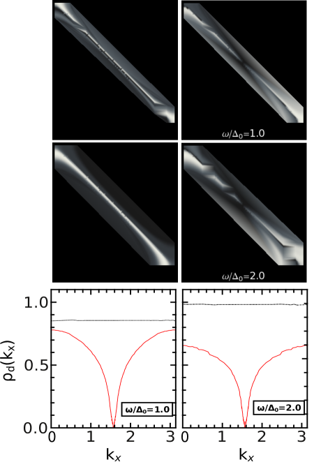
Figure 6: (Colour online) Top (Middle) Panels: Plot of the momentum distribution of the defect density $\rho_{d}({\mathbf{k}})$ (where $\mathbf{k}=k_{x}\hat{x}+k_{y}\hat{y}$) as a function of $k_{x}$ (abscissas) and $k_{y}$ (ordinates) after a full drive cycle for s-wave [left panels] and d-wave [right panels] pairing symmetries. The drive frequencies are specified in the inset of the right column. In these plots, lighter shades represent higher quasiparticle excitation densities. The abscissas of the top and middle panels have the same range and scale as those of the bottom panels viz. $k_{x}\in[0,\pi]$, and have been omitted for brevity. The ordinates of the top and middle panels plot $k_{y}\in[0,\pi]$ in a similar manner, and have been omitted as well.
Bottom Panel: Plot of the momentum distribution of the defect density (black dotted line for s-wave and red solid line for d-wave) along the Fermi surface in the first quadrant ($k_{x},k_{y}\geq 0$) as a function of $k_{x}$, with $k_{y}$ chosen to lie on the Fermi surface given by $f_{\bf k}=\cos{k_{x}}+\cos{k_{y}}-\mu_{0}=0$ $\forall k_{x}$. These plots clearly demonstrate the dip in the momentum distribution at the node for d-wave pairing. Analogous dips occur at other three quadrants at the position of the other nodes of $\Delta({\mathbf{k}})$. In all of these plots, $\mu_{0}=0.01$, $\Delta_{0}=0.1$.

4 Analytical computation of the magnetization

In this section, we obtain an analytical understanding of the behaviour of the magnetization or fermion density at the gap edge, i.e. at $f_{\mathbf{k}}=0$, after a drive cycle in the high-frequency limit. We note that from Refs. [39] and [42], we can conclude that the non self-consistent dynamics for a two-level system described in section 2 is affected by two phenomena, Landau-Zener tunnelling and the Stückelberg phase. In what follows, we derive an analogous picture for the s-wave BCS fermions with the self-consistency condition. The calculation is carried out here for s-wave superfluids but can be easily generalized to other pairing symmetries.

We begin with  (21) and (22), yielding

$$\dot{u}_{\mathbf{k}}(t) = -i\left[\epsilon_{\mathbf{k}}-\mu(t)\right]u_{\mathbf{k}}(t)-i\Delta(t)v_{\mathbf{k}}(t),$$

$$\dot{v}_{\mathbf{k}}(t) = i\left[\epsilon_{\mathbf{k}}-\mu(t)\right]v_{\mathbf{k}}(t)-i\Delta^{\ast}(t)u_{\mathbf{k}}(t),$$

$$\Delta(t) = g\sum_{{\mathbf{k}}}u^{\ast}_{\mathbf{k}}(t)v_{\mathbf{k}}(t).$$ (33)

Table 1: Values of system dynamical variables $u_{\mathbf{k}}(t)$, $v_{\mathbf{k}}(t)$, $s_{\mathbf{k}}(t)$, $b_{\mathbf{k}}(t)$, and $\Delta(t)$, their time derivatives and second derivatives at $t=0-$ where the avoided crossing takes place for adiabatic initial conditions. See  (13), (21), (22) and (2) for details.

• Value		First derivative		Second derivative
  $u_{\mathbf{k}}=u^{\rm eq}_{\mathbf{k}}$		$\dot{u}_{\mathbf{k}}=-i\left(f_{\mathbf{k}}u^{\rm eq}_{\mathbf{k}}+\Delta_{0}v^{\rm eq}_{\mathbf{k}}\right)$		$\ddot{u}_{\mathbf{k}}=-\left[E^{2}({\mathbf{k}})-i\mu_{a}\omega\right]{u^{\rm eq}_{\mathbf{k}}}$
  $v_{\mathbf{k}}=v^{\rm eq}_{\mathbf{k}}$		$\dot{v}_{\mathbf{k}}=+i\left(f_{\mathbf{k}}v^{\rm eq}_{\mathbf{k}}-\Delta_{0}u^{\rm eq}_{\mathbf{k}}\right)$		$\ddot{v}_{\mathbf{k}}=-\left[E^{2}({\mathbf{k}})+i\mu_{a}\omega\right]{v^{\rm eq}_{\mathbf{k}}}$
  $s_{\mathbf{k}}=1$		$\dot{s}_{\mathbf{k}}=-if_{\mathbf{k}}$		$\ddot{s}_{\mathbf{k}}=-\left(f^{2}_{\mathbf{k}}-i\mu_{a}\omega\right)$
  $b_{\mathbf{k}}=v^{\rm eq}_{\mathbf{k}}$		$\dot{b}_{\mathbf{k}}=-i\Delta_{0}u^{\rm eq}_{\mathbf{k}}$		$\ddot{b}_{\mathbf{k}}=-\Delta_{0}v^{\rm eq}_{\mathbf{k}}\left(\Delta_{0}+2f_{\mathbf{k}}\right)$
  $\Delta=\Delta_{0}$		$\dot{\Delta}=0$		$\ddot{\Delta}=-2i\Delta_{0}\mu_{a}\omega$

Defining the terms

$$s_{\mathbf{k}}(t) = \exp\left\{-i\int^{t}_{0}\mathrm{d}t^{\prime}{\left[\epsilon_{\mathbf{k}}-\mu(t^{\prime})\right]}\right\},$$

$$u_{\mathbf{k}}(t) = a_{\mathbf{k}}(t)s_{\mathbf{k}}(t),\quad v_{\mathbf{k}}(t)=b_{\mathbf{k}}(t)s^{-1}_{\mathbf{k}}(t),$$ (34)

the dynamics of the system can be rewritten as

$$\dot{a}_{\mathbf{k}} = -i\Delta(t)b_{\mathbf{k}}(t)s^{-2}_{\mathbf{k}}(t),$$

$$\dot{b}_{\mathbf{k}} = -i\Delta^{\ast}(t)a_{\mathbf{k}}(t)s^{2}_{\mathbf{k}}(t),$$ (35)

which leads to two decoupled second-order differential equations for $a_{\mathbf{k}}(t)$ and $b_{\mathbf{k}}(t)$ given by

$$\ddot{a}_{\mathbf{k}}-\left\{2i\left[\epsilon_{\bf k}-\mu(t)\right]+\frac{\dot{\Delta}(t)}{\Delta(t)}\right\}\dot{a}_{\mathbf{k}}+|\Delta(t)|^{2}a_{\mathbf{k}} = 0,$$

$$\ddot{b}_{\mathbf{k}}+\left\{2i\left[\epsilon_{\mathbf{k}}-\mu(t)\right]-\frac{\dot{\Delta}^{\ast}(t)}{\Delta^{\ast}(t)}\right\}\dot{b}_{\mathbf{k}}+|\Delta(t)|^{2}b_{\mathbf{k}} = 0.$$

The self-consistency condition can be written in terms of ${a}_{\bf k}(t)$ and $b_{\mathbf{k}}(t)$ as

$$\Delta(t)=g\exp{\left[-2i\int^{t}_{0}{\mathrm{d}}t^{\prime}\mu^{\prime}(t^{\prime})\right]}\sum_{\mathbf{k}}a^{\ast}_{\mathbf{k}}(t)b_{\mathbf{k}}(t)e^{2if_{\mathbf{k}}t},$$ (37)

where $f_{\mathbf{k}}=\epsilon_{\mathbf{k}}-\mu_{0}$ and $\mu^{\prime}(t)=\mu_{a}\sin{\omega t}$. The initial conditions for $a_{\bf k}$ and $b_{\mathbf{k}}$ can be easily obtained from those of $u_{\mathbf{k}}$ and $v_{\mathbf{k}}$ as discussed in section 2.

To obtain an analytical insight into the solution of these equations, we note that there is an avoided crossing at $t_{1{\bf k}}=t_{1}=\arcsin(f_{\mathbf{k}}/\mu_{a})/\omega$ and that $t_{1}$ approaches zero for large $\omega$ and on the Fermi surface. Further if $\omega t_{1}\ll 1$, a condition which is exactly satisfied at $f_{\mathbf{k}}=0$, we may use the Zener approximation $\mu^{\prime}(t)\approx\mu_{a}\omega t$ for $\mu(t)$ close to $t=t_{1}$ when the system traverses the avoided crossing [42, 43, 44], and restrict ourselves within the adiabatic impulse model where all excitations away from the avoided crossing are ignored [39]. From the definitions in  (4) and  (4), we can simplify  (4) to yield

$$\dot{a}_{\mathbf{k}}=-i\Delta(t)b_{\mathbf{k}}(t)e^{2i\left(f_{\mathbf{k}}t-\frac{1}{2}\mu_{a}\omega t^{2}\right)}.$$ (38)

We now assume that $\omega\gg\Delta_{0}$ and define

$$x_{\mathbf{k}} = t\sqrt{\mu_{a}\omega}-f_{\mathbf{k}}/\sqrt{\mu_{a}\omega}$$

$$\theta_{\mathbf{k}}(t) = b_{\mathbf{k}}(t)\Delta(t)/\Delta_{0}=v_{\bf k}(t)s_{\mathbf{k}}(t)\Delta(t)/\Delta_{0}.$$ (39)

We can use these definitions to simplify  (38), yielding

$$\frac{\partial a_{\mathbf{k}}}{\partial x_{\mathbf{k}}}=-i\frac{\Delta_{0}\theta_{\mathbf{k}}(x_{\mathbf{k}})}{\sqrt{\mu_{a}\omega}}e^{\frac{if^{2}_{\mathbf{k}}}{\mu_{a}\omega}}e^{-ix^{2}_{\mathbf{k}}}.$$ (40)

Thus, the amplitude $a_{\mathbf{k}}(t)$ after the system traverses an avoided crossing is approximately given by

$$\mathcal{A}^{(1)}_{\mathbf{k}}-\mathcal{A}^{(0)}_{\mathbf{k}}=-\frac{i\Delta_{0}}{\sqrt{\mu_{a}\omega}}e^{\frac{if^{2}_{\bf k}}{\mu_{a}\omega}}\int^{\infty}_{-\infty}\mathrm{d}x_{\mathbf{k}}\theta_{\mathbf{k}}(x_{\mathbf{k}})e^{-ix^{2}_{\mathbf{k}}},$$ (41)

where $\mathcal{A}^{(n)}_{\mathbf{k}}$ denotes the amplitude $a_{\mathbf{k}}$ after $N$ passages across the avoided crossings with $\mathcal{A}^{(0)}_{\mathbf{k}}$ being the initial amplitude of $a_{\bf k}$ [42, 39].

The integral in the right side of  (41) can be evaluated by contour integration whose details are charted out in the Appendix. This yields

$$\mathcal{A}^{(1)}_{\mathbf{k}} = u^{\rm eq}_{\bf k}-\sqrt{\frac{\pi\Delta^{2}_{0}}{\mu_{a}\omega}}e^{i\left(\frac{f^{2}_{\bf k}}{\mu_{a}\omega}+\frac{\pi}{4}\right)}$$ (42)

$$\times\sum^{\infty}_{n=0}\frac{1}{n!}\frac{\left(-i\right)^{n}}{\left(4\mu_{a}\omega\right)^{n}}\frac{\partial^{2n}\theta_{\mathbf{k}}}{\partial^{2n}t}\bigg{|}_{t=t_{\bf k}},$$

where we have used $a_{\mathbf{k}}(0)=u^{\rm eq}_{\mathbf{k}}$ from  (4), and $t_{\mathbf{k}}=f_{\mathbf{k}}/(\mu_{a}\omega)$. Note that, in general, $t_{\mathbf{k}}\neq 0$ and so evaluating the modified Landau Zener probability for an arbitrary momentum will require knowledge of the system at times $t_{\mathbf{k}}$. However, $t_{\mathbf{k}}$ vanishes exactly on the Fermi surface (characterized by $f_{\mathbf{k}}=0$) and can be set to zero for all ${\mathbf{k}}$ that lie within $\mathcal{O}(\mu_{a}\omega/v_{F})$ around the Fermi surface, where $v_{F}$ is the Fermi velocity. In the rest of this section, we shall restrict ourselves to this limit.

The fermion density in momentum space $n_{{\mathbf{k}}}=2|\mathcal{B}^{(1)}_{\mathbf{k}}|^{2}=2|v_{\mathbf{k}}|^{2}$ after one passage across the avoided crossing can be obtained in terms of the modified Landau Zener probability

$$|\mathcal{B}^{(1)}_{\mathbf{k}}|^{2} = 1-|\mathcal{A}^{(1)}_{\mathbf{k}}|^{2}$$ (43)

$$= 1-\Big{[}\left(u^{\rm eq}_{\mathbf{k}}\right)^{2}+\chi_{0}|c_{\mathbf{k}}|^{2}$$

$$-2u^{\rm eq}_{\mathbf{k}}\sqrt{\chi_{0}}\times{\rm Re}\left(c_{\bf k}e^{i\kappa_{\mathbf{k}}}\right)\Big{]},$$

where we have defined

$$c_{\mathbf{k}} = \sum^{\infty}_{n=0}\frac{1}{n!}\frac{\left(-i\right)^{n}}{\left(4\mu_{a}\omega\right)^{n}}\frac{\partial^{2n}\theta_{\bf k}}{\partial^{2n}t}\bigg{|}_{t=t_{\mathbf{k}}},$$

$$\kappa_{\mathbf{k}} = \frac{f^{2}_{\mathbf{k}}}{\mu_{a}\omega}+\frac{\pi}{4},\quad\chi_{0}=\frac{\pi\Delta^{2}_{0}}{\mu_{a}\omega}.$$ (44)

Noting that for $\omega\gg f_{\mathbf{k}}$, $\kappa_{\mathbf{k}}\sim\pi/4$, and approximating

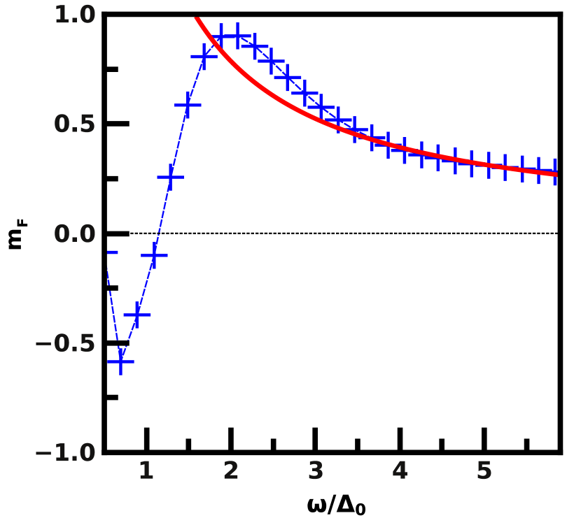
Figure 7: (Colour Online) Numerical plots (blue crosses) of $m_{F}$ as a function of $\omega$. The system parameters are the same as in  figure 1. The red solid line indicates the analytical result obtained in  (53).

$$c_{\mathbf{k}}\approx\sum^{\infty}_{n=0}\frac{1}{n!}\frac{\left(-i\right)^{n}}{\left(4\mu_{a}\omega\right)^{n}}\frac{\partial^{2n}\theta_{\mathbf{k}}}{\partial^{2n}t}\bigg{|}_{t=0},$$ (45)

one finally gets an expression for the modified Landau-Zener probability

$$|\mathcal{B}^{(1)}_{\mathbf{k}}|^{2} = \left(v^{\rm eq}_{\mathbf{k}}\right)^{2}-\chi_{0}|c_{\mathbf{k}}|^{2}+u^{\rm eq}_{\bf k}\sqrt{2\chi_{0}}{\rm Re}\left[\left(1+i\right)c_{\mathbf{k}}\right]$$

Each of the terms in the sum of  (45) can be obtained from table 1 and higher order derivatives thereof using  (2) and either  (4) or  (4) at $t=0$. We now define $P_{\mathbf{k}}$ to be the traditional Landau Zener probability for the non self-consistent case [43, 44, 42] viz.

$$P_{\mathbf{k}}=e^{-\chi_{0}}.$$ (47)

Now, we can write $|\mathcal{B}^{(1)}_{{\mathbf{k}}}|^{2}=(P_{\mathbf{k}}/2)e^{\gamma_{\mathbf{k}}}$, where

$$\gamma_{\mathbf{k}} = \chi_{0}+\ln\Big{\{}2\left(v^{\rm eq}_{\mathbf{k}}\right)^{2}-2\chi_{0}|c_{\mathbf{k}}|^{2}$$ (48)

$$+2u^{\rm eq}_{\mathbf{k}}\sqrt{2\chi_{0}}{\rm Re}\left[\left(1+i\right)c_{\mathbf{k}}\right]\Big{\}}$$

for large $\omega$. We now investigate regions close to the Fermi surface by simplifying  (45), retaining only the terms up to $n=1$ in the expansion. This yields

$$c_{\mathbf{k}}\approx\frac{v^{\rm eq}_{\bf k}}{2}\left[1+\frac{i\chi_{0}}{2\pi}\left(1+\frac{2f_{\bf k}}{\Delta_{0}}\right)\right],$$ (49)

where we have used expressions from table 1. Taking the approximation for $c_{\mathbf{k}}$ in eq (49), substituting its value into  (43), and retaining lowest contributing orders of $\chi_{0}$ yields

$$|\mathcal{B}^{(1)}_{\mathbf{k}}|^{2}\approx|v^{\rm eq}_{\mathbf{k}}|^{2}\left[1+\frac{\chi^{1/2}_{0}}{\sqrt{2}}\frac{u^{\rm eq}_{\mathbf{k}}}{v^{\rm eq}_{\mathbf{k}}}\right].$$ (50)

The occupation amplitude $\mathcal{B}^{(1)}_{\mathbf{k}}$ is realized after the first passage across the avoided crossing and when the second passage begins. The passage starts when the adiabatic energy equals the BCS gap $\Delta_{0}$. The adiabatic energies are given by $E({\mathbf{k}};t)=\pm\sqrt{\left[f_{\mathbf{k}}-\mu_{a}\sin{\omega t}\right]^{2}+|\Delta_{0}|^{2}}$, which is $E({\mathbf{k}})$ from (13), with $\mu_{0}$ replaced by $\mu_{0}+\mu_{a}\sin{\omega t}$. The passage ends when the velocity of the adiabatic energy vanishes, i.e when $\dot{E}({\mathbf{k}};t)=0$ at $t=\pi/\omega$ or half a period. Thus, $|\mathcal{B}^{(1)}_{\mathbf{k}}|^{2}$ is the fermion density after half a drive cycle. After one complete period i.e two passages across the avoided crossing, the fermion density in the adiabatic impulse limit is given by [39]

$$|\mathcal{B}^{(2)}_{\mathbf{k}}|^{2} = 4|\mathcal{B}^{(1)}_{\mathbf{k}}|^{2}\left(1-|\mathcal{B}^{(1)}_{\mathbf{k}}|^{2}\right)\sin^{2}[\Phi_{\rm st}]$$ (51)

$$\simeq 2|\mathcal{B}^{(1)}_{\mathbf{k}}|^{2}\left(1-|\mathcal{B}^{(1)}_{\mathbf{k}}|^{2}\right)$$

$$= 2\bigg{[}\left(u^{\rm eq}_{\mathbf{k}}v^{\rm eq}_{\mathbf{k}}\right)^{2}\left(1-\frac{\chi_{0}}{2}\right)$$

$$+u^{\rm eq}_{\mathbf{k}}v^{\rm eq}_{\mathbf{k}}\left(|u^{\rm eq}_{\mathbf{k}}|^{2}-|v^{\rm eq}_{\mathbf{k}}|^{2}\right)\sqrt{\frac{\chi_{0}}{2}}\bigg{]},$$

where in the second line, we have used the fact that the Stückelberg phase $\Phi_{\rm st}\to\pi/4$ for large $\omega$ [39]. Thus the magnetization $m_{\mathbf{k}}^{(2)}$ after one period (or two passages across the avoided crossing) can be evaluated using  (24) and (51), yielding

$$m^{(2)}_{\mathbf{k}} \simeq 1-4\left(1-\frac{\chi_{0}}{2}\right)\left(u^{\rm eq}_{\mathbf{k}}v^{\rm eq}_{\mathbf{k}}\right)^{2}+\sqrt{8\chi_{0}}u^{\rm eq}_{\mathbf{k}}v^{\rm eq}_{\mathbf{k}}m^{\rm eq}_{\mathbf{k}},$$

where $m^{\rm eq}_{\mathbf{k}}$, the equilibrium magnetization, is given by $m^{\rm eq}_{\mathbf{k}}=1-2|v^{\rm eq}_{\mathbf{k}}|^{2}$. Thus, on the Fermi surface, where all approximations used to arrive at this result are clearly valid, one obtains, using $u_{F}^{\rm eq}(v_{F}^{\rm eq})=u_{{\bf k}={\mathbf{k}}_{F}}^{\rm eq}(v_{{\bf k}={\mathbf{k}}_{F}}^{\rm eq})={1\over\sqrt{2}}$,

$$m_{F}\equiv m^{(2)}_{{\bf k}={\mathbf{k}}_{F}}=m_{0}\frac{\Delta_{0}}{\omega},\quad m_{0}=\frac{\pi\Delta_{0}}{2\mu_{a}}.$$ (53)

Here, ${\mathbf{k}}_{F}$ denotes the momentum vector on the Fermi surface. We note that $m_{F}$ does not depend on the orientation of ${\mathbf{k}}$ on the Fermi surface. This is a consequence of the s-wave symmetry of the superfluid order parameter and is not going to be present for other pairing symmetries.

Thus, we find that the frequency dependence of the magnetization (or equivalently the fermion density) is $m_{F}\sim\omega^{-1}$. The magnetization drops off at the same manner as the non self-consistent case (i.e the driven Ising model where $m\sim\omega^{-1}$ can be obtained from the Landau Zener formula). The constant $m_{0}$ which decides the rate of the decrease of $m_{F}$ with $\omega$, however, is different in the two cases. In the non self-consistent case, $\Delta$ is always constant and so $c_{\mathbf{k}}={1\over\sqrt{2}}$ exactly as yielded by  (45). Thus, $m^{(2)}\approx 2\chi_{0}$ to lowest order which is four times its value for the self-consistent case. We note here that although we have concentrated on $m_{F}$, our results are expected to be accurate for all $m_{\mathbf{k}}$ for which $t_{1}\simeq 0$ and $f_{\bf k}\ll\mu_{a}$. The generalization of this treatment to $N$ periods seems to be difficult due to the necessity of taking into account multiple Stuckelberg phases and we leave this issue for a possible future study.

To check the accuracy of the analytical result, we compare (53) with numerical results for the magnetization on the Fermi surface after one drive period for a $144\times 144$ square optical lattice which is very close to half filling ($\mu_{0}=0.01$) with $\mu_{a}=\Delta_{0}=0.1$. At each time step of the numerics, the Fermi surface was strobed with a tolerance $\sim\mu_{a}\omega$. In the limit of $f_{\mathbf{k}}\ll\mu_{a}$, the variation of $m_{F}$ is expected to be small within this region of the Brillouin zone and an average over all momenta inside this region should yield values close to that predicted by  (53). The agreement, as shown in  figure 7, is quite good for $\omega\geq 3\Delta_{0}$ but poor for smaller $\omega/\Delta_{0}$ where some of the approximations made in this section are clearly violated.

5 Discussion

Experimental verification of our work will require generation of a time-dependent chemical potential. This can be easily done by turning on an additional trap with oscillatory time dependence leading to a potential of the form $\kappa(t)r^{2}/2$. Both the confining and the additional trap potentials are to be made wide-enough so that the atoms residing at the centre of the trap feel an almost spatially constant chemical potential. Such traps can be easily designed in current experimental setups [46]. To verify our theory, we propose momentum distribution measurements as done recently for fermions on a honeycomb lattice by Tarruell, Greif, Uehlinger, Jotzu and Esslinger [45]. A comparison of momentum distribution of the superfluid fermions before and the after the dynamics could be used to measure the momentum distribution of the defects generated during the drive. Our theory predicts that this momentum distribution would depend on the pairing symmetry of the superfluid and its pattern would be qualitatively similar to that showing in  figure 6 for $s-$ and $d_{x^{2}-y^{2}}-$wave superfluids.

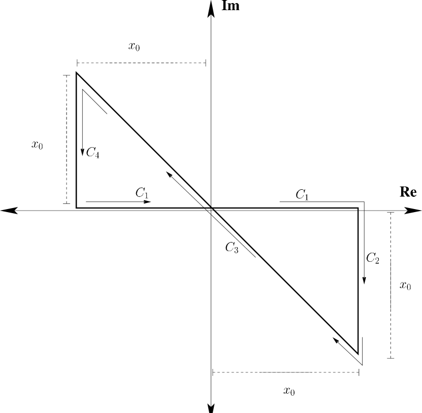
Figure 8: Contour $\mathrm{C}=\mathrm{C}_{1}+\mathrm{C}_{2}+\mathrm{C}_{3}+\mathrm{C}_{4}$ used for evaluating the integral in ((41)) in the complex $x$-plane. The path traversed is indicated by arrows, and the contour consists of two isosceles right angled triangles of height $x_{0}$ laid out as shown above.

In conclusion, we have studied the non-equilibrium periodic dynamics of Fermi superfluids in the BCS regime within a self-consistent mean-field theory. We have shown that proper incorporation of the self-consistency condition is crucial for understanding the dynamic properties of such systems. This is particularly highlighted by studying the behaviour of the effective magnetization $m(t)$ (or equivalently $n_{0}$) which shows qualitatively different behaviour for Fermi superfluids (which obey self-consistent BCS equations) and Ising or Kitaev spin models (whose properties are governed by BCS-like equations without the self-consistency condition). We have also studied the behaviour of defect density, it’s momentum distribution, and the residual energy for such dynamics. In particular, we find that the momentum distribution of the defect density bears a signature of the pairing symmetry of such superfluids. Finally, we have provided an analytical derivation of the frequency dependence $m_{F}$ at the end of one drive cycle in the limit of large drive frequency and have shown that $m_{F}\sim 1/\omega$ for $\omega\gg\Delta_{0}$.

Appendix A

Here we provide details of the evaluation of  (41) in  section 4. The integral in the right side of  (41) can be evaluated by following the contour $\mathrm{C}=\mathrm{C}_{1}+\mathrm{C}_{2}+\mathrm{C}_{3}+\mathrm{C}_{4}$ in the complex plane as shown in  figure 8. Along the path $\mathrm{C}_{1}$, we have $\mathrm{d}z=\mathrm{d}x$ and $\exp{(-iz^{2})}=\exp{(-ix^{2})}$. Along the path $\mathrm{C}_{2}$, we have $\mathrm{d}z=-i\mathrm{d}y$ and $\exp{(-iz^{2})}=\exp{[-i(x_{0}-iy)^{2}]}=\exp{[-i(x^{2}_{0}-y^{2})]}\times\exp{(-2x_{0}y)}$, an integrand that vanishes when $x_{0}\rightarrow\infty$. Along the path $\mathrm{C}_{3}$, we have $\mathrm{d}z=(1-i)\mathrm{d}x$ and $\exp{(-iz^{2})}=\exp{(-2x^{2})}$. Finally, the integrand vanishes along path $\mathrm{C}_{4}$ in a way similar to that along $\mathrm{C}_{2}$. Since the contour $\mathrm{C}$ does not enclose any poles, Cauchy’s theorem yields $\oint_{\mathrm{C}}\mathrm{d}z\theta_{\mathbf{k}}(z)e^{-iz^{2}}=0$. Thus, taking the limit $x_{0}\rightarrow\infty$,

$$\int^{\infty}_{-\infty}\mathrm{d}x_{\mathbf{k}}\theta_{\mathbf{k}}(x_{\mathbf{k}})e^{-ix^{2}_{\mathbf{k}}}=$$

$$\left(1-i\right)\int^{\infty}_{-\infty}\mathrm{d}x_{\mathbf{k}}\theta_{\mathbf{k}}\left[\left(1-i\right)x_{\mathbf{k}}\right]e^{-2x^{2}_{\bf k}}.$$ (54)

Performing a Taylor expansion of $\theta_{\mathbf{k}}$,

$$\theta_{\mathbf{k}}(x_{\mathbf{k}})=\sum^{\infty}_{n=0}\frac{x^{n}_{\bf k}}{n!}\frac{\partial^{n}\theta_{\mathbf{k}}}{\partial^{n}x_{\bf k}}\bigg{|}_{x_{\mathbf{k}}=0},$$ (55)

and substituting this into the right side of  (A) after the transformation $x_{\mathbf{k}}\rightarrow(1-i)x_{\mathbf{k}}$, each term in the sum can be evaluated using Gaussian integrals, yielding

$$\int^{\infty}_{-\infty}\mathrm{d}x_{\mathbf{k}}\theta_{\mathbf{k}}\left[\left(1-i\right)x_{\mathbf{k}}\right]e^{-2x^{2}_{\mathbf{k}}}=$$

$$\sqrt{\frac{\pi}{2}}\sum^{\infty}_{n=0}\frac{1}{n!}\frac{\left(-i\right)^{n}}{\left(4\mu_{a}\omega\right)^{n}}\frac{\partial^{2n}\theta_{\mathbf{k}}}{\partial^{2n}t}\bigg{|}_{t=t_{\bf k}},$$ (56)

Using the above result, we evaluate  (A) and hence  (41). This yields (42) used in section 4.

References

References

• [1] Bloch I, Dalibard J and Zwerger W 2008 Rev. Mod. Phys. 80 885.
• [2] Jin D S, Ensher J, Matthews M R, Wieman C E and Cornell E A 1996 Phys. Rev. Lett. 77 420.
• [3] Giorgini S, Pitaevskii L P, Stringari S 2008 Rev. Mod. Phys. 80 1215.
• [4] De Marco B and Jin D S 1999 Science 285 1703. Schreck F, Khaykovich L, Corwin K L, Ferrari G, Bourdel T, Cubizolles J and Salomon C 2001 Phys. Rev. Lett. 87 080403. Truscott A K, Strecker K E, McAlexander W I, Partridge G B and Hulet R G 2001 Science 291 2570.
• [5] Bulgac A, McNeil Forbes M and Magierski P 2012 Lecture Notes in Physics 836 305-373.
• [6] See, for example, Giorgini, Pitaevski and Stringari [3], as well as Bulgac, McNeil Forbes and Magierski [5], for a detailed account.
• [7] O’Hara K M, Hemmer S L, Gehm M E, Granade S R and Thomas J E 2002 Science 298 2179.
• [8] Bartenstein M, Altmeyer A, Riedl S, Jochim S, Chin C, Hecker Denschlag J and Grimm R 2004 Phys. Rev. Lett. 92 203201.
• [9] Chin C, Bartenstein M, Altmeyer A, Riedl S, Jochim S, Denschlag J H and Grimm R, 2004 Science 305 1128.
• [10] Zwierlein M W, Abo-Shaeer J R, Schirotzek A, Schunck C H and Ketterle W 2005 Nature 435 1047.
• [11] Leggett A J 2006 Rev. Mod. Phys. 73 307. Leggett A J 1980 Modern Trends in the Theory of Condensed Matter ed A Pekalski and R Przystawa (Springer-Verlag, Berlin). Nozi res P and Schmitt-Rink S 1985 J. Low Temp. Phys. 59 195. Sa de Melo C A R, Randeria M and Engelbrecht J R 1993 Phys. Rev. Lett. 71 3202. Randeria M 1994 Bose-Einstein Condensation ed A Griffin, D Snoke and S Stringari (Cambridge University Press, Cambridge).
• [12] Holland M, Kokkelmans S J J M F, Chiofalo M L and Walser R 2001 Phys. Rev. Lett. 87 120406. Timmermans E, Furuya K, Milonni P W and Kerman A K 2001 Phys. Lett.A 285 228. Pieri P, Pisani L and Strinati G C 2004 Phys. Rev.B 70 094508.
• [13] Petrov D S, Salomon C and Shlyapnikov G V 2004 Phys. Rev. Lett. 93 090404. Stajic J, Milstein J N, Chen Q J, Chiofalo M L, Holland M J, and Levin K 2004 Phys. Rev.A 69 063610. Haussmann R, Rantner W, Cerrito S and Zwerger W 2007 Phys. Rev.A 75 023610.
• [14] Ohashi Y and Griffin A 2002 Phys. Rev. Lett. 89 130402. Bruun G M and Pethick C 2004 Phys. Rev. Lett. 92 140404 (2004). Romans M W J and Stoof H T C 2006 Phys. Rev.A 74 053618. Roy A 2012 Eur. Phys. J. Plus 127 34.
• [15] Carlson J, Chang S -Y, Pandharipande V R and Schmidt K E 2003 Phys. Rev. Lett. 91 050401. Astrakharchik G E, Boronat J, Casulleras J and Giorgini S 2004 Phys. Rev. Lett. 93, 200404. Juille O 2007 New J. Phys. 9 163.
• [16] Menotti C, Pedri P and Stringari S, 2002 Phys. Rev. Lett. 89 250402. Stringari S 2004 Europhys. Lett. 65 749.
• [17] For details of studies of vortex dynamics, see, for example, Bloch, Dalibard and Zwerger [1].
• [18] Babadi M, Pekker D, Sensarma R, Georges A and Demler E 2009 Non-equilibrium dynamics of interacting Fermi systems in quench experiments Preprint arXiv:0908.3483.
• [19] Minguzzi A, Ferrari G and Castin Y 2001 Eur. Phys. J. D 17 49.
• [20] Polkovnikov A, Sengupta K, Silva A and Vengalattore M 2011 Rev. Mod. Phys. 83 863.
• [21] Dziarmaga J 2010 Advances in Physics 59 1063.
• [22] Damski B 2005 Phys. Rev. Lett. 95 035701.
• [23] Zurek W H, Dorner U and Zoller P 2005 Phys. Rev. Lett. 95 105701.
• [24] Polkovnikov A 2005 Phys. Rev.B 72 161201(R).
• [25] Sen D, Sengupta K and Mondal S 2008 Phys. Rev. Lett. 101 016806.
• [26] Mondal S, Sen D and Sengupta K 2008 Phys. Rev.B 78 045101.
• [27] Rigol M, Dunjko V and Olshanii M 2008 Nature 452 854.
• [28] Das A 2010 Phys. Rev.B 82 172402. Bhattacharyya S, Das A and Dasgupta S 2012 Phys. Rev.B 86 054410.
• [29] Polkovnikov A and Gritsev V 2008 Nat. Phys. 4 477. De Grandi C and Polkovnikov A 2010 Lecture Notes in Physics vol 802, ed A Das, A Chandra and B. K. Chakrabarti (Heidelberg:Springer).
• [30] Kolodrubetz M, Pekker D, Clark B K and Sengupta K 2012 Phys. Rev.B 85 100505(R).
• [31] Trefzger C and Sengupta K 2011 Phys. Rev. Lett. 106 095702. Dutta A, Trefzger C and Sengupta K 2012 Phys. Rev.B 86 085140.
• [32] Das A and Moessner R 2012 Switching the Anomalous DC Response of an AC-driven Quantum Many-body system Preprint arXiv:1208.0217.
• [33] Simon J, Bakr W, Ma R, Tai M E, Preiss P and Greiner M 2011 Nature 472 307.
• [34] Greiner M, Mandel O, Esslinger T, Hänsch T W and Bloch I 2002 Nature 415, 39. Orzel C, Tuchman A K, Fenselau M L, Yasuda M and Kasevich M A 2001 Science 291 2386. Kinoshita T, Wenger T and Weiss D S 2006 Nature 440 900. Sadler L E, Higbie, J M, Leslie S R, Vengalattore M and Stamper-Kurn D M 2006 Nature 443 312.
• [35] Bakr W S, Peng A, Tai M E, Ma R, Simon J, Gillen J I, Fölling S, Pollet L and Greiner M 2010 Science 329, 547.
• [36] Kim K, Chang M -S, Korenblit S, Islam R, Edwards E E, Freericks J K, Lin G -D, Duan L -M and Monroe C 2010 Nature 465, 590 (2010). K. Kim et al 2011 New J. Phys. 13 105003.
• [37] Friedenauer A, Schmitz H, Glueckert J T, Porras D and Schaetz T 2008 Nat. Phys. 4, 757.
• [38] Mondal S, Pekker D, and Sengupta K 2012 Dynamic freezing of strongly correlated ultracold bosons Preprint arXiv:1204.6331.
• [39] Shevchenko S N, Ashhab S and Nori F 2012 Physics Reports 492 1.
• [40] Das A (in preperation).
• [41] Yukalov V I 2009 Phys. Rev.A 79 052117.
• [42] Wittig C 2005 J. Phys. Chem.B 109 8428.
• [43] Landau L D 1932 Physics of the Soviet Union 2 46.
• [44] Zener C 1932 Proc. R. Soc.London Ser. A 137 696.
• [45] Tarruell L, Greif D, Uehlinger T, Jotzu G and Esslinger T 2012 Nature 483 302-305.
• [46] See, for example, Greiner, Mandel, Esslinger, Hänsch and Bloch [34].