Network Coordination and Synchronization in a Noisy Environment with Time Delays

Abstract

We study the effects of nonzero time delays in stochastic synchronization problems with linear couplings in complex networks. We consider two types of time delays: transmission delays between interacting nodes and local delays at each node (due to processing, cognitive, or execution delays). By investigating the underlying fluctuations for several delay schemes, we obtain the synchronizability threshold (phase boundary) and the scaling behavior of the width of the synchronization landscape, in some cases for arbitrary networks and in others for specific weighted networks. Numerical computations allow the behavior of these networks to be explored when direct analytical results are not available. We comment on the implications of these findings for simple locally or globally weighted network couplings and possible trade-offs present in such systems.

I Introduction

Since the classic works by Kalecki [1] and Frisch & Holme [2] on the emergence of macro-economical patterns (business and economics cycles), it has been well-established that time delays occurring on microscopic scales can have profound effects on the global response of complex systems. Among other early key results were the works by Hutchinson [3] and May [4], showing that time delays can have fundamental impact on logistic growth in population dynamics [5]. The importance of time delay becomes even more explicit in interacting individual- or agent-based models [6, 7, 8, 9, 10], where the delays can correspond to time scales in the interactions (e.g. transmission delays) or to time scales of the local decision and execution by the individuals. In this paper, we consider the simplest – yet fundamental – model for such networked systems, taking into consideration the effects of the network topology and couplings, noise, and time delays [11]. This paper provides an extended account of our recent Letter [11], providing more details, generalizations and comparisons to certain weighted networks, and considering different types of delays.

In network synchronization [12], coordination, or consensus problems [6], individuals or entities represented by nodes in the network attempt to adjust their local state variables (e.g., pace, load, phase, or orientation) in a decentralized fashion. (In this paper, we use the terms synchronization, coordination, and consensus synonymously in this broader sense.) Nodes interact or communicate only with their local neighbors in the network, often with the intention to improve global performance. These couplings can be represented by directed or undirected, weighted or unweighted links. Applications of the corresponding models range from physics, biology, computer science to control theory, including synchronization problems in distributed computing [13], symbolic dynamics [14], congestion control in communication networks [15, 16, 17, 18, 6] and in vehicular traffic [19, 20], flocking animals [21, 22, 23], bursting neurons [24], and cooperative control of vehicle formation [25].

Synchronization, coordination, or consensus in complex networks cuts across numerous fields that address global behavior through decentralized local actions facilitated by sparse interactions. There has already been much investigation into the efficiency and optimization of synchronization [12, 26, 27, 28, 29] in weighted [30, 15, 16] and directed [6, 31, 32] topologies. Because of limitations in communication, transportation, processing, or cognitive resources, the local information on the state of the network neighborhood may not always be current, nor is it even given for the same instant at a past time for all components. These time delays can have drastic effects on system behavior [7] and further complicate predictability of the network’s global performance.

The impact of time delays on stochastic differential equations involving a single stochastic variable, with recent applications to postural sway [33, 34], stick balancing at a fingertip [36, 35], and the scaling of congestion window in internet protocols [37], have been investigated in the past two decades [38, 39, 40, 41]. Here, we focus on the interplay of network topology, couplings, noise, and time delays. Our motivation is to understand how network-connected individuals contribute to global goals by performing delayed actions and/or using delayed information facilitated by local interactions in a noisy environment.

The phenomena of spontaneous synchronization, coordination, or consensus arise in a variety of disciplines [16, 12, 6, 7]. For example, it describes the consensus that arises in bird flocks as each bird makes velocity adjustments to match the group, which is crucial in accomplishing such tasks as avoiding predators [23, 22]. Similarly, it can be applied to a collection of autonomous vehicles working cooperatively to carry out a task [18]. Risk can be managed without central governance in uncertain environments through the synchronicity or spontaneous cooperation of individuals. This appears in economics when considering stock trades [42]; in ecology there is the reward of reproduction and the danger of predation for chirping cicadas and flashing fireflies [43]. While there are adversarial relationships between individual participants, there are still mutual benefits (predictive insight or bodily protection) from the collective behavior. Massively parallel and distributed computing schemes require synchronization across processors [13, 44, 45, 46] in order to avoid diverging progressions of simulation time but must be balanced with the cost of communication. Synchronization of coupled phase oscillators [47] (the Kuramoto model [48]) has many applications, recently to spatial patterns in flashing microfluidic arrays [49] and to circuits comprised of optomechanical arrays [50]. In neural networks, time delays critically affect the synchronization of excitatory fronts [51, 52, 53]. All these examples are instances of a group coming to consensus [6] without an omniscient global operator. They fundamentally rely on the communication between individuals, which may be (and often is) sent through noisy channels [39, 40, 41].

I.1 The Model

In the model we consider here, the state of each node $i$ is described by a local scalar state variable $h_{i}$. In stochastic network coordination/consensus problems, nodes locally adjust their state in an attempt to match that of their neighbors through linear couplings in the presence of noise. However, they react to the information or signal received from their neighbors with some time lag, and the evolution of the states of the nodes is governed by the differential time-delay equations

$$\partial_{t}h_{i}(t)=-\sum_{j}C_{ij}[h_{i}(t-\tau^{\rm o}_{i})-h_{j}(t-\tau^{\rm o}_{i}-\tau^{\rm tr}_{ij})]+\eta_{i}(t)\;.$$ (1)

Here, $C_{ij}$ is the coupling strength between nodes $i$ and $j$, and $\eta_{i}$ is the noise present at node $i$, satisfying $\langle\eta_{i}(t)\eta_{j}(t^{\prime})\rangle=2D\delta_{ij}\delta(t-t^{\prime})$, where $D$ is the noise intensity. In general, the time delays can be heterogeneous, depending on the properties and network locations of both nodes: $\tau^{\rm o}_{i}$ is the local delay at node $i$, corresponding to processing, cognitive, or execution delays, while $\tau^{\rm tr}_{ij}$ is the transmission delay between nodes $i$ and $j$. Without the noise term, the above equation is often referred to as the (deterministic) consensus problem [18, 6] on the respective network. In this sense, the networked agents try to coordinate or reach an agreement or balance regarding a certain quantity of interest.

A standard measure of synchronization, coordination, or consensus in a noisy environment is the width [15, 13]

$$\langle w^{2}(t)\rangle=\biggl{\langle}\frac{1}{N}\sum_{i=1}^{N}[h_{i}(t)-\bar{h}(t)]^{2}\biggr{\rangle}\;,$$ (2)

where $\bar{h}(t)=(1/N)\sum_{i=1}^{N}h_{i}(t)$ is the global average of the local state variables and $\langle\ldots\rangle$ denotes an ensemble average over the noise. A network is “synchronizable” if it asymptotically reaches a steady state with a finite width, i.e. $\langle w(\infty)\rangle<\infty$. When the network is well synchronized (or coordinated), the values $h_{i}$ for all nodes are near the global mean $\bar{h}$ and the width is small.

I.2 Coordination without Time Delays

Without time delays, Eq. (1) takes the form

$$\partial_{t}h_{i}(t)=-\sum_{j}C_{ij}[h_{i}(t)-h_{j}(t)]+\eta_{i}(t)=-\sum_{j}\Gamma_{ij}h_{j}(t)+\eta_{i}(t)$$ (3)

where $\Gamma_{ij}=\delta_{ij}\sum_{l}C_{il}-C_{ij}$ is the network Laplacian. Eq. (3) is a multivariate Ornstein-Uhlenbeck process [54] and is also referred to as the Edwards-Wilkinson process [55] on a network [13, 15]. Starting from a flat initial profile $\{h_{i}(0)=0\}_{i=1}^{N}$ for symmetric couplings, one can show that the width evolves as [54]

$$\langle w^{2}(t)\rangle=\frac{D}{N}\sum_{k=1}^{N-1}\frac{(1-e^{-2\lambda_{k}t})}{\lambda_{k}}\;,$$ (4)

where $\lambda_{k}$, $k=0,1,2,\ldots,N-1$, are the eigenvalues of the network Laplacian. Note that as a result of measuring the local state variables $h_{i}$ from the mean $\bar{h}$ in Eq. (2), the singular contribution of $\lambda_{0}=0$ (associated with the uniform mode) automatically cancels out from the sum in Eq. (4). Thus, a finite connected network is always synchronizable with steady-state width

$$\langle w^{2}(\infty)\rangle=\frac{D}{N}\sum_{k=1}^{N-1}\frac{1}{\lambda_{k}}\;.$$ (5)

In the limit of infinite network size, however, network ensembles with a vanishing (Laplacian) spectral gap may become unsynchronizable, depending on the details of the small-$\lambda$ behavior of the density of eigenvalues [12, 13, 15]. This type of singularity is common in purely spatial networks (in particular, in low dimensions) where the relevant response functions and fluctuations diverge in the long-wavelength (small-$\lambda$) limit [13, 56]. In complex networks [58, 57, 59, 60] these singularities are typically suppressed as a result of sufficient amount of randomness in the connectivity pattern generating a gap or “pseudo” gap. [61, 13, 26, 62, 63, 64].

As is also clear from Eq. (5), synchronization or coordination can be arbitrarily improved in this case of no time delays, e.g., by uniformly increasing the coupling strength by a factor of $\sigma>1$, resulting in $C_{ij}\rightarrow\sigma C_{ij}$ ($\lambda_{k}\rightarrow\sigma\lambda_{k}$) and yielding

$$\langle w^{2}(\infty)\rangle_{\sigma}=\frac{1}{\sigma}\langle w^{2}(\infty)\rangle_{\sigma=1}\;.$$ (6)

The stronger the effective coupling $\sigma$ (e.g., achieved by more frequent communications in real networks), the better the synchronization; the width is a monotonically decreasing function of $\sigma$.

II Uniform Local Time Delays

We first consider the case with symmetric coupling $C_{ij}=C_{ji}$ when transmission delays are negligible ($\tau^{\rm tr}_{ij}=0$) and local delays are uniform ($\tau^{o}_{i}\equiv\tau$). Then Eq. (1) is governed by a single uniform time delay [11]

$$\partial_{t}h_{i}(t)=-\sum_{j=1}^{N}C_{ij}[h_{i}(t-\tau)-h_{j}(t-\tau)]+\eta_{i}(t)=-\sum_{j=1}^{N}\Gamma_{ij}h_{j}(t-\tau)+\eta_{i}(t)\;.$$ (7)

This equation has a similar form to that of Eq. (3) but with the inclusion a delay $\tau$.

II.1 Eigenmode Decomposition and Scaling

By diagonalizing the symmetric network Laplacian $\Gamma$, the above set of equations of motion decouples into separate modes

$$\partial_{t}\tilde{h}_{k}(t)=-\lambda_{k}\tilde{h}_{k}(t-\tau)+\tilde{\eta}_{k}(t)\;,$$ (8)

where $\lambda_{k}$ ($k=0,1,2,\ldots,N-1$) are the eigenvalues of the network Laplacian, and $\tilde{h}_{k}$ and $\tilde{\eta}_{k}$ are the time-dependent components of the state and noise vectors, respectively, along the $k$-th eigenvector. Thus, the amplitude $\tilde{h}_{k}$ of each mode (with the exception of the uniform mode with $\lambda_{0}=0$) is governed by the same type of stochastic delay-differential equation

$$\partial_{t}\tilde{h}(t)=-\lambda\tilde{h}(t-\tau)+\tilde{\eta}(t)\;,$$ (9)

with $\lambda>0$, where we temporarily drop the index $k$ of the specific eigenmode for transparency and to streamline notation.

While the above stochastic delay-differential equation has an exact stationary solution for the stationary-state variance [38, 40], we first review the formal solution [65, 11] which provides some insights and connections between the solutions of the underlying characteristic equation and the existence (and the scaling) of the stationary-state fluctuations of the stochastic problem. The formal solution can also be applied to more general linear (or linearized) coordination problems with multiple time delays [66], and can serve as the starting point to extract the asymptotic behavior [67] near the singular points (synchronization boundary).

Performing standard Laplace transform on Eq. (9) [with $\hat{h}(s)=\int_{0}^{\infty}e^{-st}\tilde{h}(t)dt$], the characteristic equation associated with its homogeneous (deterministic) part becomes

$$g(s)\equiv s+\lambda e^{-s\tau}=0\;.$$ (10)

As shown in Appendix A, (with $h(t)\equiv 0$ for $t\leq 0$) the time-dependent fluctuations can be written formally as

$$\langle\tilde{h}^{2}(t)\rangle=\sum_{\alpha,\beta}\frac{-2D(1-e^{(s_{\alpha}+s_{\beta})t})}{g^{{}^{\prime}}(s_{\alpha})g^{{}^{\prime}}(s_{\beta})(s_{\alpha}+s_{\beta})}\;.$$ (11)

Hence, they remain finite (i.e., a stationary distribution exists) if

$${\rm Re}(s_{\alpha})<0\;,$$ (12)

for all $\alpha$, where $s_{\alpha}$, $\alpha=1,2,\ldots$, are the solutions of the characteristic equation, Eq. (10), on the complex plane. We can explicitly make the simplification

$$\langle\tilde{h}^{2}(\infty)\rangle=\sum_{\alpha,\beta}\frac{-2D}{g^{{}^{\prime}}(s_{\alpha})g^{{}^{\prime}}(s_{\beta})(s_{\alpha}+s_{\beta})}=\sum_{\alpha,\beta}\frac{-2D}{(1+\tau s_{\alpha})(1+\tau s_{\beta})(s_{\alpha}+s_{\beta})}\;.$$ (13)

Eq. (10) is perhaps the oldest and most well-known (transcendental) characteristic equation from the theory of delay-differential equations [18, 2, 68, 5], with the linear stability analysis of numerous nonlinear systems reducing to this one. It has an infinite number of (in general, complex) solutions for $\tau>0$ and the condition in Eq. (12) holds if

$$\lambda\tau<\pi/2\;.$$ (14)

Long-time dynamics of the solution of Eq. (9) is governed by the zero(s) of Eq. (10) with the largest real part. In particular, for $\lambda\tau\leq 1/e$, the zero with the largest real part is purely real, hence no sustained oscillations occur [Fig. 1(a)]. For $1/e<\lambda\tau<\pi/2$, all zeros have imaginary parts (including the ones with the largest real part) and are arranged symmetrically about the real axis. This results in persistent oscillations that do not diverge so long as condition (14) is satisfied, as shown in Fig. 1(b).

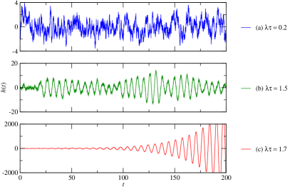
Figure 1: (Color online) Time evolution of an individual mode obtained by numerically integrating Eq. (9) with $\lambda$$=$$1$, $D$$=$$1$, and $\Delta t$$=$$0.001$ for several delays chosen to show the various behaviors across the separating/critical points $\lambda\tau$$=$$1/e$ and $\pi/2$; (a) $\lambda\tau$$=$$0.2<1/e$, (b) $1/e<\lambda\tau$$=$$1.5<\pi/2$, and (c) $\lambda\tau$$=$$1.7>\pi/2$.

The first pair of zeros to acquire positive real parts are the two with smallest imaginary parts. Once the product $\lambda\tau$ fails to satisfy the condition in Eq. (14), the oscillation amplitude grows in time [Fig. 1(c)]. Specific time series for $\langle h^{2}(t)\rangle$ are shown in Fig. 2, where the real parts of solutions have become positive for delays $\tau=1.60$ and $2.00$ but remain negative for the rest.

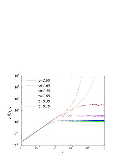
Figure 2: (Color online) Time series of the fluctuations of a single mode ($\lambda$$=$$1$) averaged over $10^{4}$ realizations of noise (with $D$$=$$1$) by numerically integrating Eq. (9) with $\Delta t$$=$$0.01$ for different delays (from bottom to top in increasing order of $\tau$).

To obtain the general scaling form of the fluctuations in the stationary state, we define $z_{\alpha}\equiv\tau s_{\alpha}$ ($\alpha=1,2,\ldots$). One can easily see that the new variables $z_{\alpha}$ are the corresponding solutions of the scaled characteristic equation,

$$z+\lambda\tau e^{-z}=0\;,$$ (15)

and hence can only depend on $\lambda\tau$, i.e. $z_{\alpha}=z_{\alpha}(\lambda\tau)$. Thus,

$$s_{\alpha}(\lambda,\tau)=\frac{1}{\tau}z_{\alpha}(\lambda\tau)\;.$$ (16)

Substituting this into Eq. (13) yields

$$\langle\tilde{h}^{2}(\infty)\rangle=D\tau f(\lambda\tau)\;,$$ (17)

where

$$f(\lambda\tau)=\sum_{\alpha,\beta}\frac{-2}{(1+z_{\alpha})(1+z_{\beta})(z_{\alpha}+z_{\beta})}$$ (18)

is the scaling function. This scaling [Eq. (17)] is illustrated by plotting $\langle\tilde{h}^{2}(\infty)\rangle/\tau$ vs $\lambda\tau$, fully collapsing the data for different $\tau$ values (with fixed noise intensity $D$) [Fig. 3].

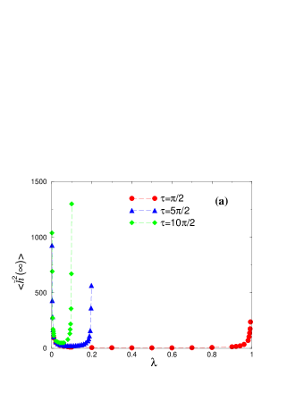
Figure 3: (Color online) (a) Steady-state fluctuations of an individual mode as a function of $\lambda$ obtained by numerical integration of Eq. (9) for several delays with $D$$=$$1$ and $\Delta t$$=$$0.01$. (b) Scaled fluctuations of an individual mode and the analytic scaling function Eq. (19) (solid curve).

As mentioned earlier, Eq. (9) has an exact solution for the stationary-state variance obtained by Küchler and Mensch [38] (briefly reviewed in Appendix B), providing an exact form for the scaling function

$$f(\lambda\tau)=\frac{1+\sin(\lambda\tau)}{\lambda\tau\cos(\lambda\tau)}\;.$$ (19)

The asymptotic behavior of the scaling function near the singular points, $\lambda\tau=0$ and $\lambda\tau=\pi/2$, can be immediately extracted from the exact solution given by Eq. (19) (see also Ref. [67] for a more generalizable method),

$$f(\lambda\tau)\simeq\begin{cases}\displaystyle\frac{1}{\lambda\tau}&~{}~{}0<\lambda\tau\ll 1\\ \displaystyle\frac{4}{\pi(\pi/2-\lambda\tau)}&~{}~{}\displaystyle 0<\frac{\pi}{2}-\lambda\tau\ll 1\;.\end{cases}$$ (20)

The scaling function $f(x)$ ($x\equiv\lambda\tau$) is clearly non-monotonic; it exhibits a single minimum, at approximately $x^{*}\approx 0.739$ with $f^{*}=f(x^{*})\approx 3.06$, found through numerical minimization of Eq. (19). The immediate message of the above result is rather interesting: For a single stochastic variable governed by Eq. (9) with a nonzero delay, there is an optimal value of the “relaxation” coefficient, $\lambda^{*}=x^{*}/\tau$, at which point the stationary-state fluctuations attain their minimum value $\langle\tilde{h}^{2}(\infty)\rangle=D\tau f^{*}\approx 3.06D\tau$. This is in stark contrast with the zero-delay case (the standard Ornstein-Uhlenbeck process [54]) where $\langle\tilde{h}^{2}(\infty)\rangle=D/\lambda$, i.e., the stationary-state fluctuation is a monotonically decreasing function of the relaxation coefficient.

II.2 Implications for Coordination in Unweighted Networks

Since the eigenvectors of the Laplacian are orthogonal for symmetric couplings, the width can be expressed as the sum of the fluctuations for all non-uniform modes

$$\langle w^{2}(\infty)\rangle=\frac{1}{N}\sum_{k=1}^{N-1}\langle\tilde{h}_{k}^{2}(\infty)\rangle=\frac{D\tau}{N}\sum_{k=1}^{N-1}f(\lambda_{k}\tau)\;,$$ (21)

where $\lambda_{k}$ is the eigenvalue of the $k$th mode. Thus, condition (14) must be satisfied for every $k>0$ mode for synchronizability, or equivalently [69],

$$\lambda_{max}\tau<\frac{\pi}{2}\;.$$ (22)

The above exact delay threshold for synchronizability has some profound consequences for unweighted networks. Here, the coupling matrix is identical to the adjacency matrix, $C_{ij}=A_{ij}$, and the bounds and the scaling properties of the extreme eigenvalues of the network Laplacian are well known. In particular [70, 71],

$$\frac{N}{N-1}k_{\rm max}\leq\lambda_{\rm max}\leq 2k_{\rm max}\;,$$ (23)

where $k_{\rm max}$ is the maximum node degree in the network [i.e., $\langle\lambda_{\rm max}\rangle={\cal O}(\langle k_{\rm max}\rangle)$]. Thus, $\tau k_{\rm max}<\pi/4$ is sufficient for synchronizibility [69], while $\tau k_{\rm max}>\pi/2$ leads to the breakdown of synchronization with certainty. These inequalities imply that even a single (outlier) node with a sufficiently large degree can destroy synchronization or coordination in unweighted networks (regardless of the general trend, if any, of the tail of the degree distribution). Naturally, network realizations selected from an ensemble of random graphs with a power-law tailed degree distribution typically have large hubs, making them rather vulnerable to intrinsic network delays [18, 6]. For example, Barabási-Albert (BA) [58, 59] and uncorrelated [72, 73] scale-free (SF) networks with structural degree cut-off (yielding $\lambda_{\rm max}\sim k_{\rm max}\sim N^{1/2}$) and similarly, SF network ensembles with natural cut-off (exhibting $\lambda_{\rm max}\sim k_{\rm max}\sim N^{1/(\gamma-1)}$) for $N\gg 1$ [60, 72]), are particularly vulnerable. Thus, for any fixed delay, increasing the size of scale free networks will eventually lead to the violation of condition (22), and in turn, to the breakdown of synchronization. In contrast, the typical largest degree (hence the largest eigenvalue of the Laplacian) grows much slower in Erdős-Rényi (ER) random graphs [74], as $\lambda_{\rm max}\sim k_{\rm max}\sim\ln(N)$.

To illustrate the above finite-size dependence, we define the fraction of synchronizable networks $p_{\rm s}(\tau,N)$, which is equivalent to the probability that a randomly chosen realization of a network ensemble satisfies $\lambda_{\rm max}$$<$$\pi/2\tau$. Thus, $p_{\rm s}(\tau,N)=P_{N}^{<}(\pi/2\tau)$, where $P_{N}^{<}(x)$ is the cumulative probability distribution of the largest eigenvalue of the network Laplacian. In Fig. 4, we show the fraction of synchronizable networks for BA and ER network ensembles by employing direct numerical diagonalization of the corresponding network Laplacians and evaluating condition (22) for each realization.

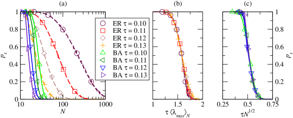
Figure 4: (Color online) The fraction of synchronizable networks $p_{s}(\tau,N)$ taken from ensembles of $10^{4}$ random constructions of ER and BA networks with $\langle k\rangle\approx 6$. (a) $p_{s}$ vs. $N$. (b) and (c) are scaled plots of the same data according to Eq. (24), for ER and BA networks, respectively.

For $N\gg 1$ the cumulative distribution for the largest eigenvalue exhibits the asymptotic scaling $P_{N}^{<}(x)\sim\phi(x/\langle\lambda_{\rm max}(N)\rangle)$ [64]. Thus, the fraction of synchronizable networks should scale as

$$p_{\rm s}(\tau,N)=P_{N}^{<}(\pi/2\tau)\sim\phi(\pi/2\tau\langle\lambda_{\rm max}(N)\rangle)=\psi(\tau\langle\lambda_{\rm max}(N)\rangle)\;.$$ (24)

In Figs. 4 (b) and (c), we demonstrate the above scaling for ER and BA networks, respectively.

Since the scaling function is known exactly [Eq. (19)], the eigenmode decomposition [Eq. (21)] allows one to evaluate the stationary width for an arbitrary network with a single uniform time delay by utilizing numerical diagonalization of the network Laplacian

$$\langle w^{2}(\infty)\rangle=\frac{D\tau}{N}\sum_{k=1}^{N-1}f(\lambda_{k}\tau)=\frac{D\tau}{N}\sum_{k=1}^{N-1}\frac{1+\sin(\lambda_{k}\tau)}{\lambda_{k}\tau\cos(\lambda_{k}\tau)}\;.$$ (25)

The optimal (minimal) width occurs when all eigenvalues of the Laplacian are degenerate so that the couplings and/or delay can be tuned to the minimum of Eq. (19). For each mode in Eq. (25), such degeneracy is present in the case of a fully-connected network with uniform couplings, optimized to $C_{ij}=x^{*}/N\tau$ ($i\neq j$) and $C_{ii}=0$. For general networks, better synchronization can be achieved when the eigenvalue spectrum is narrow relative to the range of synchronizability so that most eigenvalues can fall near the minimum of Eq. (19). We have not investigated in detail how to achieve a narrow spectrum, but strategies for doing so by tuning coupling strengths or adding/removing links have been explored by others [31, 32].

II.3 Scaling, Optimization, and Trade-offs in Networks with Uniform Delays

With the knowledge of the scaling function in Eq. (25), one also immediately obtains the width for the case of an arbitrary but uniform effective coupling strength $\sigma$, where $C_{ij}=\sigma A_{ij}$. The effective coupling strength can now be tuned for optimal synchronization. However, there is a trade-off between how well the network synchronizes and the range over which it is synchronizable. When the eigenvalue spectum is not narrow, diminishing the couplings uniformly in order to satisfy Eq. (22) may cause small eigenvalues to be pushed farther up the left divergence of the scaling function. Figure 5(a) shows this trade-off in uniform reweighting ($C_{ij}\rightarrow\sigma C_{ij}$).

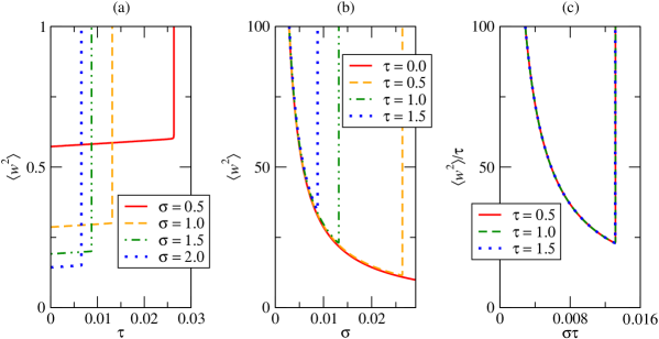
Figure 5: (Color online) Stationary-state widths obtained through numerical diagonalization and utilizing Eq. (25) for a typical BA network with $N=100$ (a) for several coupling strengths, (b) for several delays, and (c) scaled so that the nonzero delay curves collapse.

The monotonicity of these widths means that the uniform delay should always be minimized to obtain the best synchronization. The same conclusion can be drawn from Fig. 5(b), which shows that networks synchronize better and do not become unsynchronizable until greater link strengths when the delay $\tau$ is minimized. Because globally reweighting the coupling strengths corresponds to a uniform scaling of the eigenvalues, we can define the width of a network by a scaling function $F(\sigma\tau)$ (see Fig. 5(c))

$$\langle w^{2}(\infty)\rangle_{\sigma,\tau}=\frac{D\tau}{N}\sum_{k=1}^{N-1}f(\sigma\lambda_{k}\tau)=D\tau F(\sigma\tau).$$ (26)

Fluctuations from small eigenvalues dominate other contributions to the width for small $\sigma\tau$, hence the optimal value occurs near the end of the synchronizable region, where the network fails to meet condition (22).

As an alternative to varying the (effective) uniform coupling strength $\sigma$, consider a scenario where the frequency (or rate) of communication is controlled for each node according to

$$\partial_{t}h_{i}(t)=-p_{i}(t)\sum_{j=1}^{N}A_{ij}[h_{i}(t-\tau)-h_{j}(t-\tau)]+\eta_{i}(t)\;.$$ (27)

In the above scheme, $p_{i}(t)$ is a binary stochastic variable for each node, such that at each discretized time step, $p_{i}(t)=1$ with probability $p$ and $p_{i}(t)=0$ with probability $1-p$ (for simplicity, we employ uniform communication rates). The local network neighborhood remains fixed, while nodes communicate with their neighbors only at rate $p$ at each time step. As an application for trade-off, consider a system governed by the above equations and stressed by large delays, where local pairwise communications at rate $p$$=$$1$ would yield unsynchronizability, i.e., $\tau\lambda_{max}$$>$$\pi/2$ (see Fig. 6).

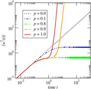
Figure 6: (Color online) Time evolution of the width obtained by numerically integrating Eq. (27) with $D$$=$$1$, $\Delta t$$=$$0.005$, and averaged over $10^{3}$ realizations of noise for several communication rates $p$ on a BA network of size $N$$=$$100$ and average degree $\langle k\rangle$$=$$6$ with $\tau\lambda_{max}$$=$$1.2\times\pi/2$.

The width diverges for one of two reasons: either communication is too frequent and the system fails to satisfy condition (22), or there is no synchronization ($p$$=$$0$) and the system is overcome by noise. However, the divergence of the width is faster in the former, accelerated by overcorrections made by each node due to the delay. With an appropriate reduction in the communication rate, the width reaches a finite steady state, recovering synchronizability, as can be seen in Fig. 6. Decreasing the frequency of communication can counter-intuitively allow a network to become synchronizable for delays and couplings that would otherwise cause the width to diverge.

II.4 Coordination and Scaling in Weighted Networks

For the case of uniform delays, we compare two cases: networks with weights that have been normalized locally by node degree and networks with weights that are globally uniform. The couplings for local weighting are defined as $C_{ij}=\sigma A_{ij}/k_{i}$ (a common weighting scheme in generalized synchronization problems [12]), while for uniform couplings $C_{ij}=\sigma A_{ij}/\langle k\rangle$. In turn, the weighted (or normalized) Laplacian becomes $\Gamma=\sigma K^{-1}L$ where $K$ is the diagonal matrix with node degrees on its diagonal, $K_{ij}=\delta_{ij}k_{i}$, and $L$ is the graph Laplacian, $L_{ij}\equiv\delta_{ij}\sum_{l}A_{il}-A_{ij}=\delta_{ij}k_{i}-A_{ij}$. Similarly, for uniform couplings, the corresponding Laplacian becomes $\Gamma=\sigma\langle k\rangle^{-1}L$. Note that the overall coupling strength (communication cost) is the same in both cases, $\sigma\sum_{ij}A_{ij}/k_{i}=\sigma\sum_{ij}A_{ij}/\langle k\rangle=\sigma N$.

In the locally-weighted case, the eigenvalue spectrum of $K^{-1}L$ is known to be confined within the interval $[0,2]$ [75], so any network of this class will be synchronizable, provided $\sigma\tau<\pi/4$. With globally uniform weighting, the increase of $\lambda_{max}$ with $N$ will lead to fewer synchronizable networks as $N$ grows (holding $\langle k\rangle$ constant).

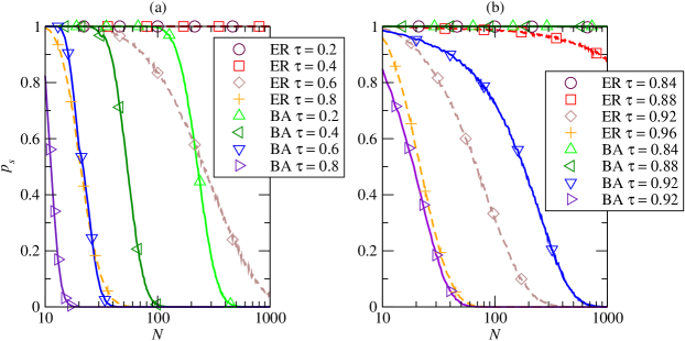
Figure 7: (Color online) Fraction of synchronizable networks for (a) uniform global weights and (b) local weights for the same ensemble of networks used in Fig. 4.

Figure 7(a) shows that it is more likely for an ER network to be synchronizable than a BA network of the same size $N$ when the couplings are weighted uniformly by $\langle k\rangle$ (with all ER networks remaining synchronizable over the range of $N$ for the two smallest delays). However, this is not always the case when couplings are weighted locally by node degree (Fig. 7(b)), although nearly all of these networks remain synchronizable over the delays in Fig. 7(a). The behavior of the width for typical networks is shown in Fig. 8 to compare the effects of these two normalizations.

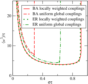
Figure 8: (Color online) Scaled widths simulated with $\Delta t$$=$$0.01$ of a typical BA and a typical ER network, each of size $N$$=$$100$ and with $\langle k\rangle$$=$$6$.

In both the BA and ER case, synchronization is better and is maintained for longer delays when the coupling strengths are weighted locally by node degree.

III Multiple Time Delays

To generalize the basic model, we now allow for a distinction in transmission and processing time delays. In this case, Eq. (1) becomes

$$\partial_{t}h_{i}(t)=-\sum_{j}C_{ij}[h_{i}(t-\tau_{\rm o})-h_{j}(t-\tau_{\rm o}-\tau_{\rm tr})]+\eta_{i}(t)$$ (28)

where the local delay $\tau_{\rm o}$ and the transmission delay $\tau_{\rm tr}$ are the same for all nodes and links, respectively. Although the synchronizability condition and steady state width cannot be determined in a closed form for arbitrary networks as is the case of Eq. (7), focusing on special cases does offer insight.

III.1 Fully-Connected Networks

Consider the case of a fully-connected network of size $N$ with uniform link strengths $\sigma$, where the local state variables evolve according to

$$\partial_{t}h_{i}(t) =-\frac{\sigma}{N-1}\sum_{j\neq i}[h_{i}(t-\tau_{o})-h_{j}(t-\tau)]+\eta_{i}(t)=-\frac{\sigma}{N-1}\sum_{j\neq i}[h_{i}(t-\gamma\tau)-h_{j}(t-\tau)]+\eta_{i}(t)$$

$$=-\frac{\sigma}{N-1}\sum_{j\neq i}[h_{i}(t-\tau)-h_{j}(t-\tau)]+\sigma h_{i}(t-\tau)-\sigma h_{i}(t-\gamma\tau)+\eta_{i}(t)$$

$$=-\frac{\sigma}{N-1}\sum_{j}\Gamma_{ij}h_{j}(t-\tau)+\sigma h_{i}(t-\tau)-\sigma h_{i}(t-\gamma\tau)+\eta_{i}(t)$$ (29)

where $\tau\equiv\tau_{\rm o}+\tau_{\rm tr}$, $\gamma\equiv\tau_{\rm o}/\tau$ and $\Gamma_{ij}=\delta_{ij}N-1$. Normalizing the global coupling with $1/(N-1)$ assures that the coupling cost per node remains constant and the region of synchronization remains finite in the limit of $N\to\infty$. Using the fact that the graph Laplacian of the complete graphs has a single, nonzero eigenvalue $N$ [which is ($N$$-$$1$)-fold degenerate], each non-uniform mode (associated with fluctuations about the mean) obeys

$$\partial_{t}\tilde{h}(t)=-\sigma\tilde{h}(t-\gamma\tau)-\frac{\sigma}{N-1}\tilde{h}(t-\tau)+\tilde{\eta}(t)\;.$$ (30)

As in the case of uniform delays, we perform a Laplace transform on the deterministic part to obtain the characteristic polynomial and equation,

$$g(s)\equiv s+\frac{\sigma}{N-1}e^{-\tau s}+\sigma e^{-\gamma\tau s}=0\;.$$ (31)

Note that for $N=2$, the region of stability/synchronizability can be obtained analytically [66], and for completeness we show it in Fig. 9 in the $(\tau_{\rm o},\tau)$ plane. In this simple case of two coupled nodes, the synchronization boundary is monotonic, and the local delay is dominant: There is no singularity (for any finite $\tau_{\rm tr}$) as long as $\sigma\tau_{o}<1/2$ [66], while for any $\tau_{\rm tr}$, there is a sufficiently large $\tau_{o}$ resulting in the breakdown of synchronization.

For $N\geq 3$, the phase diagram (region of synchronizability) can be obtained numerically by tracking the zeros of the characteristic equation Eq. (31) (i.e., identifying when their real parts switch sign) shown in Fig. 9. Note that keeping track of infinitely many complex zeros of the characteristic equations would be an insurmountable task. Instead, in order to identify the stability boundary of the system, one only needs to know whether all solutions have negative real parts. This test can be done by employing Cauchy’s argument principle [76, 77] (see Appendix C for details).

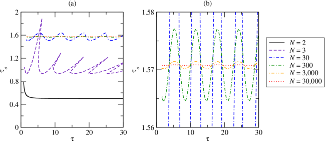
Figure 9: (Color online) Phase diagram (synchronization boundary) for fully-connected networks with uniform coupling strength $\sigma/(N-1)$ in the $(\tau_{\rm o},\tau)$ plane. (Here, without loss of generality due to scaling, we used $\sigma$$=$$1$.) (a) All system sizes (for $N$$\geq$$300$ they are essentially indistinguishable from the $N$$=$30,000 case at these scales); (b) system sizes $N$$=$$30$, 300, 3,000, 30,000 in an enlarged region for visibility. With the exception of the analytically solvable case of $N$$=$$2$ [66], the synchronization boundaries, corresponding to stability limits, were obtained from the analysis of the zeros of Eq. (31).

Similar to the $N$$=$$2$ case, the local delay is always dominant, i.e., there are critical values of $\sigma\tau_{\rm o}$ above/below which the system is unsynchronizable/synchronizable for any $\tau_{\rm tr}$. [These critical values approach $\pi/2$ as $N\to\infty$, since in this case Eqs. (30) and (31) reduce to the familiar forms of Eqs. (9) and (10), respectively, with the known analytic threshold.] The behavior with the overall delay $\tau=\tau_{\rm o}+\tau_{\rm tr}$, however, is more subtle: There is a range of $\tau_{o}$ where varying $\tau$ yields reentrant behavior with alternating synchronizable and unsynchronizable regions (as can be seen by considering suitably chosen horizontal cuts for fixed $\tau_{\rm o}$ in Fig. 9). Thus, in this region (for fixed local delays $\tau_{\rm o}$), stabilization of the system can also be achieved by increasing the transmission delays.

In the special case $\gamma=0$, the network is always synchronizable for all $N$ and the width can be obtained exactly (see Appendix B.2.b),

$$\langle w^{2}(\infty)\rangle=\frac{1}{N}\sum_{k=1}^{N-1}\langle\tilde{h}_{k}^{2}(\infty)\rangle=\frac{D(N-1)}{N}\frac{\alpha+\frac{\sigma}{N-1}\sinh(\alpha\tau)}{\alpha[\sigma+\frac{\sigma}{N-1}\cosh(\alpha\tau)]}$$ (32)

with $\alpha=\sigma\sqrt{1-1/(N-1)^{2}}$, as shown in Fig. 10.

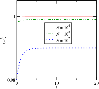
Figure 10: (Color online) Analytic results for stationary-state widths for fully-connected networks of several sizes for the special case $\gamma$$=$$0$ [Eq. (32)]. Here, $D$$=$$1$ and $\sigma$$=$$1$.

For $\tau=\tau_{\rm tr}\rightarrow\infty$, the above expression becomes

$$\langle w^{2}(\infty)\rangle=\frac{D(N-1)}{N}\frac{1}{\sigma\sqrt{1-1/(N-1)^{2}}}\;.$$ (33)

III.2 Locally Weighted Networks

Now we consider Eq. (28) with specific locally weighted couplings (already utilized for uniform local time delays in Sec.II.D), $C_{ij}=\sigma A_{ij}/k_{i}$. The set of differential equations then have the form

$$\partial_{t}h_{i}(t) =-\frac{\sigma}{k_{i}}\sum_{j}A_{ij}[h_{i}(t-\gamma\tau)-h_{j}(t-\tau)]+\eta_{i}(t)$$

$$=-\frac{\sigma}{k_{i}}\sum_{j}L_{ij}h_{j}(t-\tau)+\sigma h_{i}(t-\tau)-\sigma h_{i}(t-\gamma\tau)+\eta_{i}(t)$$

$$=-\sigma\sum_{j}\Gamma_{ij}h_{j}(t-\tau)+\sigma h_{i}(t-\tau)-\sigma h_{i}(t-\gamma\tau)+\eta_{i}(t)\;,$$ (34)

where $\sigma$ controls the coupling strength and $\Gamma=K^{-1}L$ is now the locally weighted network Laplacian ($K_{ij}=\delta_{ij}k_{i}$, and $L_{ij}=\delta_{ij}\sum_{l}A_{il}-A_{ij}=\delta_{ij}k_{i}-A_{ij}$). Diagonalization yields

$$\partial_{t}\tilde{h}_{k}(t)=\sigma(1-\lambda_{k})\tilde{h}_{k}(t-\tau)-\sigma\tilde{h}_{k}(t-\gamma\tau)+\tilde{\eta}_{k}(t)$$ (35)

where $\lambda_{k}$ is the eigenvalue of the $k$th mode of the normalized graph Laplacian $K^{-1}L$. Figure 11 shows the evolutions of a particular mode with delays on either side of the critical delay.

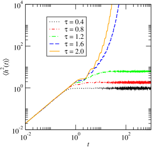
Figure 11: (Color online) Time series of the fluctuations of a single mode for several delays obtained from numerical integration of Eq. (35) with $\gamma$$=$$0.5$, $\lambda$$=$$1.8$, $D$$=$$1$, and $\Delta t$$=$$0.01$, averaged over $10^{3}$ realizations of the noise ensemble.

The characterisitic equation for the $k$th mode is then

$$g_{k}(s)=s+\sigma(\lambda_{k}-1)e^{-\tau s}+\sigma e^{-\gamma\tau s}=0\;.$$ (36)

Defining the new scaled variable $z=\tau s$, this equation becomes

$$z+(\sigma\tau)(\lambda_{k}-1)e^{-z}+(\sigma\tau)e^{-\gamma z}=0\;.$$ (37)

Hence, the solutions of the original characteristic equation depends on $\sigma$ and $\tau$ in the form of $s_{k\alpha}=\tau^{-1}z_{k\alpha}(\sigma\tau)$. Although the scaling function of the width in the case of locally normalized couplings with two time delays cannot be expressed in a closed form, the general scaling behavior is identical to Eq. (26) [as follows from the formal solution shown in Appendix D, Eq. (83)], i.e., $\langle w^{2}(\infty)\rangle_{\sigma,\tau}=D\tau F(\sigma\tau)$. The corresponding scaling behavior and scaling collapse, obtained from numerical integration of Eq. (34), are shown in Fig. 12.

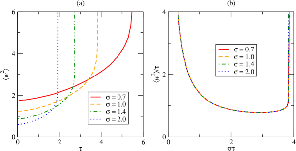
Figure 12: (Color online) Comparison of (a) the widths and (b) the scaled widths for several coupling strengths $\sigma$ on a typical locally weighted BA network of size $N$$=$$100$ and $\langle k\rangle\approx 6$ for $\gamma$$=$$0.2$; simulated with $D$$=$$1$ and $\Delta t$$=$$0.001$.

The stability/synchronization boundary was again determined by employing Cauchy’s argument principle [76, 77], applied separately for each mode (Appendix C). Figure 13 shows the most important eigenvalues to determine synchronizability: the greatest restriction to the critical delay $\tau_{c}=(\tau_{\rm o}+\tau_{\rm tr})_{c}$ for a given $\gamma$ belongs to either the smallest or largest eigenvalues.

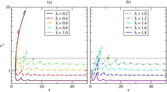
Figure 13: (Color online) Synchronization boundaries for several modes with (a) $\lambda_{k}\leq 1$ and (b) $\lambda_{k}\geq 1$ of a weighted network, obeying Eq. (35) and determined by analyzing the zeros of Eq. (37).

An alternative presentation is given in Fig. 14, which shows that it is not always the same eigenvalue that consistently limits synchronizability for all values of $\gamma$; rather it is the eigenvalue that falls on the lowest point on the boundary curve.

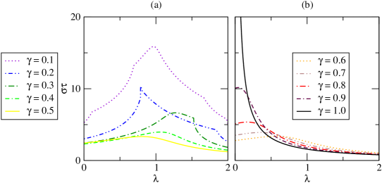
Figure 14: (Color online) Synchronization boundaries determined by analyzing the zeros of Eq. (37) for various delay ratios $\gamma$, shown separately for (a) $\gamma\leq 0.5$ and (b) $\gamma\geq 0.6$.

The contributions of a few example modes to the width are shown in Fig. 15(a). Note that the order of divergences is not the same as the ordered eigenvalues, in accordance with Fig. 13. The contributions of a single mode for various values of $\gamma$ is shown in Fig. 15(b). Since it is $\tau_{\rm o}$ that has a greater impact on whether or not a network can synchronize, larger total delays $\tau$ are tolerated for smaller $\gamma$ since more of the delay comes from transmission.

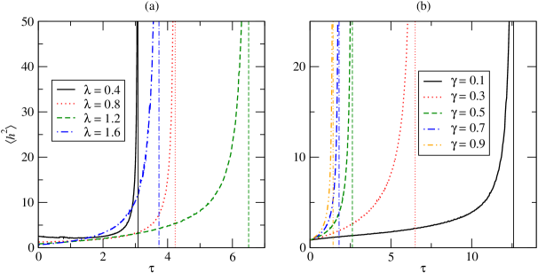
Figure 15: (Color online) Width contributions for (a) several modes with $\gamma=0.3$ and (b) several delay ratios with $\lambda=1.2$, found by numerically integrating Eq. (35) with $D$$=$$1$ and $\sigma$$=$$1$. The vertical lines correspond to the stability limits obtained from the analyses of the zeros of Eq. (36) with the same $\lambda$.

Because of the great sensitivity of $\langle h^{2}\rangle$ on $\Delta t$ near the divergence for longer delays, an adaptive algorithm was implemented, which would halve $\Delta t$ until consecutive runs agreed within 1%.

With this understanding of the underlying modes, let us return to synchronization of the entire system. Incorporating all relevant eigenvalues results in the synchronization boundary shown in Fig. 16(a) for several representative networks.

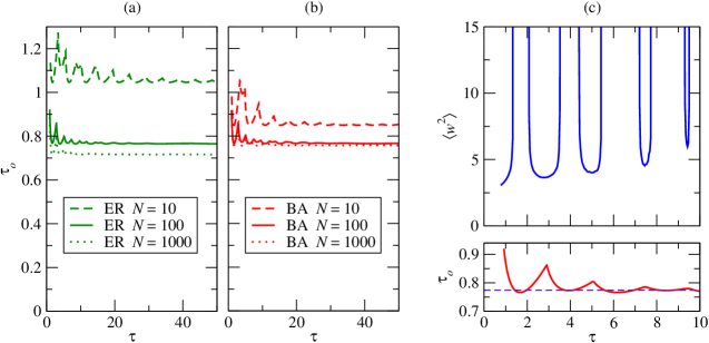
Figure 16: (Color online) Synchronization boundaries for typical (a) ER and (b) BA networks of several sizes with locally weighted couplings. The boundaries are found by numerical diagonalization and examining each mode through Eq. (36). (c) Widths along a slice of constant $\tau_{o}$$=$$0.77$ for the same $N$$=$$100$ BA network used in (b). For stability comparison, the boundary is shown below with the slice indicated.

The cut for a carefully chosen local delay in Fig. 16(b) shows the previously mentioned reentrant behavior as the transmission delay is increased. Note that the optimal width within each synchronizable region worsens with larger delay, so that while synchronizability can be recovered with increasing $\tau_{tr}$, better synchronization is possible by decreasing $\tau_{tr}$. To compare the contribution of modes within the synchronizable regime, consider again the two topologies of BA and ER graphs. For fixed $\gamma$, Fig. 17 shows that a BA graph remains synchronizable for larger delays than a ER graph when the link strengths are weighted by node degree.

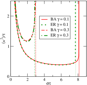
Figure 17: (Color online) The scaling functions of a typical locally weighted BA network and a typical ER network for two delay ratios, with both networks of size $N$$=$$100$, found by numerically integrating Eq. (34) with $D$$=$$1$ and $\Delta t$$=$$0.001$. The vertical lines correspond to the stability limits obtained from the analyses of the zeros of Eqs. (37).

However, the ER graph synchronizes slightly better for the majority of the time that it is synchronizable. Here it is not the topology but the ratio $\gamma$ that has the most drastic effect.

When $\gamma<1$, the mode corresponding to $\lambda_{0}=0$ includes self-interaction terms and has the critical delay

$$\tau_{c}(\lambda=0)=\frac{\pi}{1+\gamma}\frac{1}{\displaystyle\left|\cos\left(\pi\frac{1-\gamma}{1+\gamma}\right)\right|}.$$ (38)

While the uniform mode does not contribute to the width because $\bar{h}$ is removed from the state of the network (see Appendix D), a diverging mean can introduce egregious truncation errors into the numerical integration if $\bar{h}$ diverges exponentially while the width remains finite. Fortunately, this can be avoided by simulating the network in the subspace lacking the zero mode by removing the mean from each time slice. Since the uniform mode is not allowed propagate, it does not cause any problem with finite precision. The locations of the zeros’ real parts for Eq. (37) are tracked again using Cauchy’s argument principle (see Appendix C).

III.3 Arbitrary Couplings and Multiple Delays

When there are multiple time delays involved in the synchronization or coordination process, in general, one cannot diagonalize the underlying system of coupled equations. This happens to be the case for the scenario with two types of time delay [Eq. (28)] on unweighted (or globally weighted) graphs (as opposed to specific locally-weighted ones discussed in Sec. III.B). First, we briefly present a generally applicable method to determine the region of synchronizability/stability computationally [76, 77]. For arbitrary couplings $C_{ij}$, the deterministic part of Eq. (28) (from which one can extract the characteristic equation) becomes

$$\partial_{t}h_{i}(t)=-C_{i}h_{i}(t-\tau_{\rm o})+\sum_{j}C_{ij}h_{j}(t-\tau)\;,$$ (39)

where $C_{i}$$=$$\sum_{l}C_{il}$ and $\tau=\tau_{\rm o}+\tau_{\rm tr}$. After Laplace transform, these equations become

$$s\hat{h}_{i}(s)=-C_{i}\hat{h}_{i}(s)e^{-s\tau_{\rm o}}+\sum_{j}C_{ij}\hat{h}_{j}(s)e^{-s\tau}\;,$$ (40)

or equivalently,

$$\sum_{j}\left(s\delta_{ij}+C_{i}\delta_{ij}e^{-s\tau_{\rm o}}-C_{ij}e^{-s\tau}\right)\hat{h}_{j}(s)=0\;.$$ (41)

Hence, non-trivial solutions of the above system of equations require

$$\det M(s)=0\;,$$ (42)

where

$$M_{ij}(s)=s\delta_{ij}+C_{i}e^{-s\tau_{\rm o}}\delta_{ij}-C_{ij}e^{-s\tau}\;.$$ (43)

Stability or synchronizability requires that ${\rm Re}(s)$$<$$0$ for all solutions of the above (transcendental) characteristic equation [Eq. (42)]. To identify the stability boundary of this coupled system, one does not need to know and determine the (infinitely many) complex solutions of the characteristic equation, but only whether all solutions have negative real parts. To test that, one again can employ the argument principle [76, 77] (Appendix C). Note that the above method can be immediately generalized to arbitrary heterogeneous (local and transmission) time delays. To compare synchronizability with locally weighted couplings of the same cost [Eq. (34)], here, we considered $C_{ij}=\sigma A_{ij}/\langle k\rangle$. The results are shown in Fig. 18. The synchronization boundary was determined using the above scheme, while the width was obtain by numerically integrating Eq. (28). Not only does local reweighting of the coupling strength improve synchronization, but it also extends the region of synchronizability.

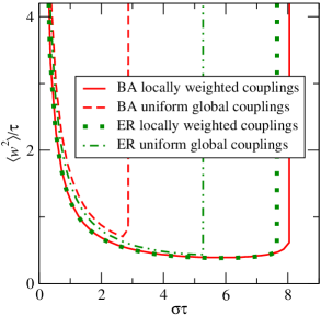
Figure 18: (Color online) Scaled width curves for a typical BA network compared to those of a typical ER network of size $N=100$ with $\langle k\rangle\approx 6$ and $D=1$, determined by numerically integrating Eq. (28) for the two types of coupling schemes with $\gamma=0.1$ and $\Delta t=0.01$.

IV Summary

Through our investigations we have explored the impact and interplay of time delays, network structure, and coupling strength on synchronization and coordination in complex interconnected systems. Here, we considered only linear couplings, already yielding a rather rich phase diagram and response. While nonlinear effects are crucial in all real-life applications [9, 51, 52, 53], linearization and stability analysis about the synchronized state yields equations analogous to the ones considered here [8, 10]. Hence, the detailed analysis of the linear problems can provide some insights to the complex phase diagrams and response of nonlinear problems.

For a single uniform local delay, the synchronizability of a network is governed solely by the largest eigenvalue and the time delay. This result links the presence of larger hubs to the vulnerability of the system becoming unstable at smaller delays. The quality of synchronization within the stable regime is described by the width, which can be enumerated exactly for arbitrary symmetric couplings, provided the spectrum is known. We have also established the boundaries of the region of synhronizability in terms of the delay and the overall coupling strength (associated with communication rate) and provided the general scaling behavior of the width inside this region. Our results underscored the importance of the interplay of stochastic effects, network connections, and time delays, in that how “less” (in terms of local communication efforts) can be “more” efficient (in terms of global performance).

For more general schemes with multiple time delays, we have shown how stability analysis in general delay differential equations can be applied to ascertain the synchronizability of a network. For cases where, at least in principle, eigenmode decomposition is possible, we have identified the general scaling behavior of the width within the synchronizable regime. However, in these cases it is not always the same eigenvalue that determines stability for all $\gamma$. In the non-monotonic nature of the scaling function, we see that there is a fundamental limit to how well a network can synchronize in the presence of noise. In the case when transmission and reaction are two independent and significant sources of delay, there is an additional parameter for tuning: the ratio of local delay to the total delay. By fixing the local delay and cutting across different values of the ratio, there is the possibility that the network will enter into and emerge from synchronizable regions. Understanding these influences can guide network design in order to maintain and optimize synchronization by balancing the trade-offs in internodal communication and local processing.

Appendix A Steady-state fluctuations for a single-variable stochastic delay equation

For a single (linearized) stochastic variable $h(t)$ with multiple time delays $\{\tau_{\omega}\}_{\omega=1}^{\Omega}$ and delta-correlated noise, one starts with the following general form

$$\partial_{t}h(t)=A_{0}h(t)+\sum_{\omega=1}^{\Omega}A_{\omega}h(t-\tau_{\omega})+\eta(t)\;,$$ (44)

where $\langle\eta(t)\eta(t^{\prime})\rangle$$=$$2D\delta(t-t^{\prime})$. Formally, the noise $\eta(t)$ plays the role of the inhomogeneous part of the above inhomogeneous linear first-order differential equation. Performing Laplace transformation [$\hat{h}(s)=\int_{0}^{\infty}e^{-st}h(t)dt$], the characteristic polynomial $g(s)$ (and the corresponding characteristic equation) associated with the homogeneous (deterministic) part of the above equation becomes

$$g(s)\equiv s-A_{0}-\sum_{\omega=1}^{S}A_{\omega}e^{-\tau_{\omega}s}=0\;.$$ (45)

For the initial condition $h(t)\equiv 0$ for $t\leq 0$ (which we employ throughout this paper), we can easily obtain the Laplace transformed Green’s function of Eq. (44) (i.e., the solution when $\eta(t)$ is replaced by $\delta(t-t^{\prime})$), which has the form

$$\hat{G}(s)=\frac{e^{-st^{\prime}}}{g(s)}\;.$$ (46)

Performing the inverse transform, one finds

$$G(t,t^{\prime})=\frac{1}{2\pi i}\int_{x_{0}-i\infty}^{x_{0}+i\infty}dse^{st}\hat{G}(s)=\frac{1}{2\pi i}\int_{x_{0}-i\infty}^{x_{0}+i\infty}ds\frac{e^{s(t-t^{\prime})}}{g(s)}=\Theta(t-t^{\prime})\sum_{\alpha}\frac{e^{s_{\alpha}(t-t^{\prime})}}{g^{{}^{\prime}}(s_{\alpha})}\;,$$ (47)

where $s_{\alpha}$ ($\alpha=1,2,\ldots$) are the zeros of the characteristic equation $g(s)=0$ on the complex plane [Eq. (45)]. In the above inverse transform, the infinite line of integration is parallel to the imaginary axis ($s=x_{0}$) and is chosen to be to the right of all zeros of the characteristic polynomial in order to apply the residue theorem by closing the contour with an infinite semicircle to the left of this line. Note that the Green’s function $G(t,t^{\prime})$ depends only on the variable $t-t^{\prime}$, reflecting the time translation symmetry of the problem. Utilizing the Grenn’s function, we can now formally write the general solution of Eq. (44) (for the same initial conditions) as

$$h(t)=\int_{0}^{\infty}dt^{\prime}G(t,t^{\prime})\eta(t^{\prime})=\int_{0}^{t}dt^{\prime}G(t,t^{\prime})\eta(t^{\prime})=\int_{0}^{t}dt^{\prime}\sum_{\alpha}\frac{e^{s_{\alpha}(t-t^{\prime})}}{g^{{}^{\prime}}(s_{\alpha})}\;\eta(t^{\prime})\;.$$ (48)

For more general initial conditions, see Ref. [78].

After averaging over the noise, one finds that the fluctuations of $h(t)$ are

$$\langle h^{2}(t)\rangle = \left\langle\int_{0}^{t}dt^{\prime}\eta(t^{\prime})\sum_{\alpha}\frac{e^{s_{\alpha}(t-t^{\prime})}}{g^{{}^{\prime}}(s_{\alpha})}\int_{0}^{t}dt^{\prime\prime}\eta(t^{\prime\prime})\sum_{\beta}\frac{e^{s_{\beta}(t-t^{\prime\prime})}}{g^{{}^{\prime}}(s_{\beta})}\right\rangle$$ (49)

$$= \int_{0}^{t}dt^{\prime}\int_{0}^{t}dt^{\prime\prime}\sum_{\alpha}\frac{e^{s_{\alpha}(t-t^{\prime})}}{g^{{}^{\prime}}(s_{\alpha})}\sum_{\beta}\frac{e^{s_{\beta}(t-t^{\prime\prime})}}{g^{{}^{\prime}}(s_{\beta})}\langle\eta(t^{\prime})\eta(t^{\prime\prime})\rangle$$

$$= \sum_{\alpha,\beta}\frac{1}{g^{{}^{\prime}}(s_{\alpha})g^{{}^{\prime}}(s_{\beta})}\int_{0}^{t}dt^{\prime}\int_{0}^{t}dt^{\prime\prime}\;e^{s_{\alpha}(t-t^{\prime})}e^{s_{\beta}(t-t^{\prime\prime})}2D\delta(t^{\prime}-t^{\prime\prime})$$

$$= \sum_{\alpha,\beta}\frac{2D}{g^{{}^{\prime}}(s_{\alpha})g^{{}^{\prime}}(s_{\beta})}\int_{0}^{t}dt^{\prime}\;e^{(s_{\alpha}+s_{\beta})(t-t^{\prime})}$$

$$= \sum_{\alpha,\beta}\frac{-2D(1-e^{(s_{\alpha}+s_{\beta})t})}{g^{{}^{\prime}}(s_{\alpha})g^{{}^{\prime}}(s_{\beta})(s_{\alpha}+s_{\beta})}\;.$$

As is explicit from the above equation, the zero with the largest real part of all $s_{\alpha}$ governs the long-time behavior of the stochastic variable $h(t)$. In particular, $h(t)$ reaches a stationary limit distribution for $t\to\infty$ with a finite variance if and only if ${\rm Re}(s_{\alpha})<0$ for all $\alpha$. In this case,

$$\langle h^{2}(\infty)\rangle=\sum_{\alpha,\beta}\frac{-2D}{g^{{}^{\prime}}(s_{\alpha})g^{{}^{\prime}}(s_{\beta})(s_{\alpha}+s_{\beta})}\;,$$ (50)

otherwise it diverges exponentially with time. Note that the condition for the existence of an asymptotic stationary limit distribution is the same as the one for the stability of the deterministic (homogeneous) part of Eq. (44) about the $h_{i}=0$ fixed point [5, 18].

Appendix B Exact Scaling Functions for Time Delayed Stochastic Differential Equations

Küchler and Mensch [38] obtained the analytic stationary-state autocorrelation function for the stochastic delay-differential equation,

$$\partial_{t}h(t)=ah(t)+bh(t-\tau)+\eta(t)\;,$$ (51)

with $\langle\eta(t)\eta(t^{\prime})\rangle=2D\delta(t-t^{\prime})$. Special cases (with suitably chosen coefficients $a$ and $b$) can be directly utilized for two of our special cases in our network investigations. Specifically, for (i) unweighted networks with symmetric couplings and uniform local time delays with no transmission delays and (ii) the case with only transmission delays on the complete graph, to be discussed at the end of this Appendix, in Appendix B.2.a and Appendix B.2.b, respectively. Here, we briefly present an equivalent derivation of their results, using the formalism used in our paper.

We define the stationary-state autocorrelation function as

$$K(t)=\langle h(t^{\prime})h(t^{\prime}+t)\rangle\;,$$ (52)

where it is implicitly assumed that $t^{\prime}\to\infty$. From this definition and the invariance under time translation in the stationary state, it follows that the interpretation of the autocorrelation function can be formally extended to $t$$<$$0$ by

$$K(t)=\langle h(t^{\prime})h(t^{\prime}+t)\rangle=\langle h(t^{\prime}+t)h(t^{\prime})\rangle=\langle h(t^{\prime})h(t^{\prime}-t)\rangle=K(-t)\;,$$ (53)

and also,

$$\dot{K}(t)=-\dot{K}(-t)\;.$$ (54)

As one would like to obtain a directly solvable equation of motion for the autocorrelation function, one must first find expressions for its time derivatives. Employing the equation of motion for $h(t)$ [Eq. (51)], we obtain for $t\geq 0$ that

$$\dot{K}(t) = \partial_{t}K(t)=\partial_{t}\langle h(t^{\prime})h(t^{\prime}+t)\rangle=\langle h(t^{\prime})\partial_{t}h(t^{\prime}+t)\rangle=\langle h(t^{\prime})\{ah(t^{\prime}+t)+bh(t^{\prime}+t-\tau)+\eta(t^{\prime}+t)\}\rangle$$ (55)

$$= a\langle h(t^{\prime})h(t^{\prime}+t)\rangle+b\langle h(t^{\prime})h(t^{\prime}+t-\tau)\rangle+\langle h(t^{\prime})\eta(t^{\prime}+t)\rangle$$

$$= aK(t)+bK(t-\tau)\;,$$ (56)

where in the last step we used $\langle h(t^{\prime})\eta(t^{\prime}+t)\rangle=0$ (i.e., Ito’s convention [54, 79]). The above expression, combined with the (analytic) extension of the autocorrelation function in Eq. (53), yields the condition

$$\dot{K}(0)=aK(0)+bK(\tau)\;$$ (57)

in the limit of $t\to+0$. Differentiating Eq. (56) again with respect to $t$ and exploiting the properties of Eqs. (53) and (54), we find

$$\ddot{K}(t) = a\dot{K}(t)+b\dot{K}(t-\tau)=a\dot{K}(t)-b\dot{K}(\tau-t)$$ (58)

$$= a\{aK(t)+bK(t-\tau)\}-b\{aK(\tau-t)+bK(-t)\}$$

$$= a\{aK(t)+bK(t-\tau)\}-b\{aK(t-\tau)+bK(t)\}$$

$$= (a^{2}-b^{2})K(t)\;.$$

Note that the reduction of the equation of motion of the autocorrelation function to a second order ordinary differential equation (with no delay) is a consequence of Eq. (51) having only one delay time-scale. The general solution of Eq. (58) can be written as

$$K(t)=A\cos(\omega t)+B\sin(\omega t)$$ (59)

with $\omega=\sqrt{b^{2}-a^{2}}$. From the definition of the autocorrelation function in Eq. (52) and from some of the basic properties of the Green’s function (see Appendix B.1 below for details), it also follows [38] that

$$\dot{K}(0)=\lim_{t\to 0}\partial_{t}\langle h(t^{\prime})h(t^{\prime}+t)\rangle=-D\;,$$ (60)

and from Eq. (57),

$$aK(0)+bK(\tau)=-D\;.$$ (61)

Thus, the second order ordinary differential equation Eq. (58) with conditions Eqs. (60) and (61) can now be fully solved, yielding

$$A=K(0)=D\frac{-\omega+b\sin(\omega\tau)}{\omega[a+b\cos(\omega\tau)]}\;,$$ (62)

and

$$B=\frac{\dot{K}(0)}{\omega}=-\frac{D}{\omega}\;.$$ (63)

Finally, the stationary-state variance of the stochastic variable governed by Eq. (51) can be written as

$$\langle h^{2}(t)\rangle=\langle h(t)h(t)\rangle=K(0)=D\frac{-\omega+b\sin(\omega\tau)}{\omega[a+b\cos(\omega\tau)]}\;.$$ (64)

Following the aforementioned technical detours and details in Appendix B.1, we will discuss in Appendix B.2 the applications of the above result to obtain the scaling function of the fluctuations for the individual modes in specific networks.

B.1 General properties of the autocorrelation function and the Green’s Function

From the definition of the autocorrelation function in Eq. (52) and of the Green’s function in Eq. (48), it follows that

$$K(t) = \langle h(t^{\prime})h(t^{\prime}+t)\rangle=\left\langle\int_{0}^{t^{\prime}}du\;G(t^{\prime},u)\eta(u)\int_{0}^{t^{\prime}+t}dv\;G(t^{\prime}+t,v)\eta(v)\right\rangle$$ (65)

$$= \int_{0}^{t^{\prime}}du\int_{0}^{t^{\prime}+t}dv\;G(t^{\prime},u)G(t^{\prime}+t,v)\langle\eta(u)\eta(v)\rangle=2D\int_{0}^{t^{\prime}}du\;G(t^{\prime},u)G(t^{\prime}+t,u)\;,$$

and consequently

$$\dot{K}(t) = \partial_{t}\langle h(t^{\prime})h(t^{\prime}+t)\rangle=2D\partial_{t}\int_{0}^{t^{\prime}}du\;G(t^{\prime},u)G(t^{\prime}+t,u)=2D\int_{0}^{t^{\prime}}du\;G(t^{\prime},u)\partial_{t}G(t^{\prime}+t,u)$$ (66)

$$= 2D\int_{0}^{t^{\prime}}du\;G(t^{\prime},u)(-\partial_{u})G(t^{\prime}+t,u)=-2D\int_{0}^{t^{\prime}}du\;G(t^{\prime},u)\partial_{u}G(t^{\prime}+t,u)\;.$$

Hence,

$$\dot{K}(0) = -2D\lim_{t\to 0}\int_{0}^{t^{\prime}}du\;G(t^{\prime},u)\partial_{u}G(t^{\prime}+t,u)=-2D\int_{0}^{t^{\prime}}du\;G(t^{\prime},u)\partial_{u}G(t^{\prime},u)$$ (67)

$$= -2D\int_{0}^{t^{\prime}}du\;\partial_{u}\frac{G(t^{\prime},u)^{2}}{2}=-D\{G(t^{\prime},t^{\prime})-G(t^{\prime},0)\}=-D\{1-0\}=-D\;,$$ (68)

where in the second term of the last expression above we now explicitly exploited that $G(t^{\prime},t^{\prime})=0$ and $G(t^{\prime},0)\to 0$ as $t^{\prime}\to\infty$. The former can be seen by a segment-by-segment integration and solution of Eq. (51) with a delta source $\delta(t-t^{\prime})$ in the intervals $(t-t^{\prime})\in[n\tau,(n+1)\tau]$, $n=0,1,2,\ldots$ [38]; the solution in the $[0,\tau]$ interval is particularly simple, $G(t,t^{\prime})=\exp[a(t-t^{\prime})]$. The latter property is trivial in that the magnitude of the Green’s function in the stationary state has to decay for large arguments.

B.2 Applications to Special Cases

B.2.1 Unweighted Symmetric Couplings with Uniform Local Delays

For symmetric couplings $C_{ij}$ with uniform local delays, the Laplacian $\Gamma_{ij}=\delta_{ij}\sum_{l}C_{il}-C_{ij}$ in Eq. (7) can, in principle, be diagonalized. Each mode is governed by Eq. (8), a special case of Eq. (51) with $a=0$, $b=-\lambda$, and $\omega=|b|=\lambda$ ($\lambda$ being the eigenvalue of the respective mode). From Eq. (64), the steady-state variance of each mode then reduces to

$$\langle h^{2}(\infty)\rangle=D\frac{1+\sin(\lambda\tau)}{\lambda\cos(\lambda\tau)}=D\tau\frac{1+\sin(\lambda\tau)}{\lambda\tau\cos(\lambda\tau)}=D\tau f(\lambda\tau)\;,$$ (69)

yielding the analytic scaling function for each mode

$$f(x)=\frac{1+\sin(x)}{x\cos(x)}\;,$$ (70)

with the scaling variable $x=\lambda\tau$.

B.2.2 Complete Graphs with Only Uniform Transmission Delays

The exact stationary-state variance of Eq. (51) can also be applied to complete graphs with global coupling $\sigma$, which have no local delays but do have uniform transmission delays, i.e., Eq. (30) with $\gamma=0$, translating to $a=-\sigma$, $b=-\sigma/(N-1)$ in Eq. (51). The analytic expression from Eq. (64) for the stationary-state variance for each (non-uniform) mode becomes

$$\langle h^{2}(\infty)\rangle=D\frac{\alpha+\frac{\sigma}{N-1}\sinh(\alpha\tau)}{\alpha[\sigma+\frac{\sigma}{N-1}\cosh(\alpha\tau)]}\;,$$ (71)

with $\alpha=\sqrt{a^{2}-b^{2}}=\sigma\sqrt{1-1/(N-1)^{2}}$.

Appendix C Application of Cauchy’s Argument Principle with Implementation

For an arbitrary complex analytic function $F(z)$, the number of zeros $N_{C}$ inside a closed contour $C$ (provided $F(z)$ has no poles/singularities inside $C$) is given by Cauchy’s argument principle (see, e.g., Ref. [80]):

$$N_{C}=\frac{1}{2\pi i}\oint_{C}\frac{F^{\prime}(z)}{F(z)}dz=\frac{1}{2\pi}\Delta_{C}\arg F(z)\;,$$ (72)

where $\Delta_{C}\arg F(z)$ is the winding number of $F(z)$ along the closed contour $C$. The characteristic equations studied in this paper can all be written as a sum of exponentials, hence there are no singularities. To determine the stability boundary, we follow Refs. [76, 77] and use Eq. (72) to track the number of zeros of the characteristic equations with positive real part (i.e., on the positive real half plane) by substituting Eqs. (36) and (42) for $F(z)$. We employed a numerical algorithm [76] for enumerating the winding number with adaptive step size. We restate the method here: a step of size $h$ along the contour in the direction $\hat{\iota}$ from $s$ to $s+h\hat{\iota}$ is accepted if $\theta(s,s+(h/2)\hat{\iota}<\theta(s,s+h\hat{\iota})<\epsilon=1$ where $\theta(s,s^{\prime})\equiv|{\rm arg}(\det M(s))-{\rm arg}(\det M(s^{\prime}))|{~{}\rm mod~{}}2\pi$. The subsequent step size is then $h\rightarrow\max\{2,\epsilon/\Delta\}$; unacceptable steps are retried with $h\rightarrow h/2$. The winding number is the count of the number of crossings of $\pi$ without a return in the opposite direction.

We choose the contour so that it detects the first zero to cross the imaginary axis and acquire a positive real part. Note that the mode corresponding to the zero eigenvalue allows the solution $z$$=$$0$ for Eq. (37), so the zero at the origin is ignored. This can be easily achieved by choosing the left edge of the contour to be nonzero but still very small. This method can be applied to any network structure with any delay scheme, provided the approximate general behavior of the zeros is understood.

As an example, consider the simplest system of two coupled nodes with uniform delay, which has a critical delay of $\pi/4$.

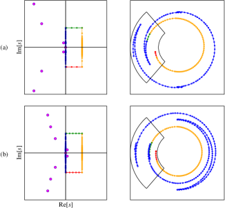
Figure 19: (Color online) Numerical integration of Eq. (72) to identify the presence of zeros in the cases of a system of two coupled nodes ($\tau_{c}$$=$$\pi/4$) for (a) $\tau$$=$$\pi/5$ and (b) $\tau$$=$$\pi/3$. The left column shows the zeros and the points sampled along the contour; the right column shows the argument of the characteristic function (angular coordinate) at these steps (radial coordinate).

Figure 19 shows two cases explored while finding the critical delay. In Fig. 19(a), $\tau=\pi/5<\tau_{c}$ and all real parts are non-positive so none fall within the contour. Tracking the argument (right column) shows that the winding number is correspondingly zero to verify that the delay is subcritical. Alternatively, $\tau=\pi/3>\pi_{c}$ in Fig. 19(b) and there do indeed exist zeros with positive real parts that fall within the contour. The argument winds around the origin twice, signaling the presence of the first two zeros to cross the imaginary axis, indicating instability.

Appendix D The Uniform Mode and the Width

D.1 Eigenmode Decomposition

In synchronization and coordination problems, it is natural to define an observable such as the width, which measures fluctuations with respect to the global mean,

$$w^{2}(t)=\frac{1}{N}\sum_{i=1}^{N}[h_{i}(t)-\bar{h}(t)]^{2}\;,$$ (73)

where $\bar{h}(t)=\sum_{i=1}^{N}h_{i}(t)$. In what follows, we show that the amplitude associated with the uniform mode of the normalized Laplacian automatically drops out from the width. (In the case of unnormalized symmetric coupling, the expression for the width simplifies to the known form.)

For our problem with two types of time delays and locally normalized couplings [Eq. (34)], decomposition along the right eigenvectors of $K^{-1}L$ facilitates diagonalization. While this normalized Laplacian is a non-symmetric matrix, its eigenvalues are all real and non-negative (with the smallest being zero, $\lambda_{0}=0$). The corresponding (normalized) right eigenvector is

$$|e_{0}\rangle=N^{-1/2}(1,1,\ldots,1)^{T}\;.$$ (74)

Note that since the normalized Laplacian is non-symmetric, the eigenvectors are not orthogonal, i.e., $\langle e_{l}|e_{k}\rangle\neq\delta_{lk}$. To ease notational burden, in this subsection we use the bra-ket notation – not to be confused with ensemble average over the noise. In this notation, $\langle\cdot|$ is a row vector and $|\cdot\rangle$ is a column vector, e.g., $\langle e_{0}|=N^{-1/2}(1,1,\ldots,1)$. Using this notation, the state vector is denoted by

$$|h(t)\rangle=(h_{1}(t),h_{2}(t),\ldots,h_{N}(t))^{T}\;,$$ (75)

while the state vector relative to the mean is

$$|h(t)-\bar{h}(t)\rangle = (h_{1}(t)-\bar{h}(t),h_{2}(t)-\bar{h}(t),\ldots,h_{N}(t)-\bar{h}(t))^{T}$$ (76)

$$= (h_{1}(t),h_{2}(t),\ldots,h_{N}(t))^{T}-\bar{h}(t)(1,1,\ldots,1)^{T}$$

$$= |h(t)\rangle-\bar{h}(t)\sqrt{N}|e_{0}\rangle=(1-|e_{0}\rangle\langle e_{0}|)|h(t)\rangle\;.$$

Employing the above formalism, the width can be written as

$$w^{2}(t)=\frac{1}{N}\sum_{i=1}^{N}[h_{i}(t)-\bar{h}(t)]^{2}=\frac{1}{N}\langle h-\bar{h}|h-\bar{h}\rangle\;.$$ (77)

Now we express the state vector as the linear combination of the eigenvectors of the underlying Laplacian,

$$|h(t)\rangle\sum_{k=0}^{N-1}\tilde{h}_{k}(t)|e_{k}\rangle\;.$$ (78)

Employing the above eigenmode decomposition, $\langle h-\bar{h}|h-\bar{h}\rangle$ can be written as

$$\langle h-\bar{h}|h-\bar{h}\rangle = \langle h|(1-|e_{0}\rangle\langle e_{0}|)^{2}|h\rangle=\langle h|(1-|e_{0}\rangle\langle e_{0}|)|h\rangle=\sum_{k=0}^{N-1}\tilde{h}_{k}(t)\langle e_{k}|\left(1-|e_{0}\rangle\langle e_{0}|\right)\sum_{l=0}^{N-1}\tilde{h}_{l}(t)|e_{l}\rangle$$ (79)

$$= \sum_{k,l=0}^{N-1}\tilde{h}_{k}(t)\tilde{h}_{l}(t)\langle e_{k}|\left(1-|e_{0}\rangle\langle e_{0}|\right)|e_{l}\rangle=\sum_{k,l=0}^{N-1}\tilde{h}_{k}(t)\tilde{h}_{l}(t)\left(\langle e_{k}|e_{l}\rangle-\langle e_{k}|e_{0}\rangle\langle e_{0}|e_{l}\rangle\right)$$

$$= \sum_{k,l\neq 0}\tilde{h}_{k}(t)\tilde{h}_{l}(t)\left(\langle e_{k}|e_{l}\rangle-\langle e_{k}|e_{0}\rangle\langle e_{0}|e_{l}\rangle\right)=\sum_{k,l\neq 0}\tilde{h}_{k}(t)\tilde{h}_{l}(t)\left(E_{kl}-E_{k0}E_{0l}\right)\;,$$

where $E_{kl}\equiv\langle e_{k}|e_{l}\rangle$. As can be seen explicitly from Eq. (79), the terms where either $k$ or $l$ are zero drop out from the sum (as $E_{00}$$=$$1$). It is also clear from Eq. (79) that $\langle h-\bar{h}|h-\bar{h}\rangle=\sum_{k\neq 0}\tilde{h}_{k}^{2}(t)$ when the underlying coupling is symmetric (and consequently the eigenvectors form an orthogonal set, $E_{kl}$$=$$\delta_{kl}$). Finally, the width can be written as

$$w^{2}(t)=\frac{1}{N}\sum_{i=1}^{N}[h_{i}(t)-\bar{h}(t)]^{2}=\frac{1}{N}\langle h-\bar{h}|h-\bar{h}\rangle=\frac{1}{N}\sum_{k,l\neq 0}\tilde{h}_{k}(t)\tilde{h}_{l}(t)\left(E_{kl}-E_{k0}E_{0l}\right)\;.$$ (80)

Note that the above result can be immediately applied to the case of symmetric coupling with no transmission delays [Eq. (7)]. There, the eigenvectors of the corresponding Laplacian form an orthogonal set, and the above expression collapses to $w^{2}(t)=\frac{1}{N}\sum_{k=1}^{N-1}\tilde{h}_{k}^{2}(t)$ [11].

D.2 Ensemble Average over the Noise

We now use the general form of the solution given in Appendix A [Eq. (48)] for the respective eigenmodes of normalized Laplacian coupling with two types of time delays [Eq. (35)], giving

$$\tilde{h}_{k}(t)=\int_{0}^{t}dt^{\prime}\sum_{\alpha}\frac{e^{s_{k\alpha}(t-t^{\prime})}}{g_{k}^{{}^{\prime}}(s_{k\alpha})}\;\tilde{\eta}_{k}(t^{\prime})\;,$$ (81)

where $s_{k\alpha}$ is the $\alpha$th solution of the $k$th mode for the characteristic equation $g_{k}(s)=0$ [Eq. (36)]. After averaging over the noise, one obtains for the two-point function

$$\langle\tilde{h}_{k}(t)\tilde{h}_{l}(t)\rangle=-2D\chi_{kl}\sum_{\alpha,\beta}\frac{(1-e^{(s_{k\alpha}+s_{l\beta})t})}{g_{k}^{{}^{\prime}}(s_{k\alpha})g_{l}^{{}^{\prime}}(s_{l\beta})(s_{k\alpha}+s_{l\beta})}\;.$$ (82)

In the stationary state, one must have ${\rm Re}(s_{k\alpha})<0$ for all $k$ and $\alpha$. Thus, the stationary state width can be written as

$$\langle w^{2}(\infty)\rangle=\lim_{t\to\infty}\frac{1}{N}\sum_{k,l\neq 0}\langle\tilde{h}_{k}(t)\tilde{h}_{l}(t)\rangle\left(E_{kl}-E_{k0}E_{0l}\right)=\frac{-2D}{N}\sum_{k,l\neq 0}\sum_{\alpha,\beta}\frac{\left(E_{kl}-E_{k0}E_{0l}\right)\chi_{kl}}{g_{k}^{{}^{\prime}}(s_{k\alpha})g_{l}^{{}^{\prime}}(s_{l\beta})(s_{k\alpha}+s_{l\beta})}\;.$$ (83)

References

- [1] M. Kalecki, Econometrica 3, 327 (1935).
- [2] R. Frisch and H. Holme, Econometrica 3, 225 (1935).
- [3] G.E. Hutchinson, Ann. N.Y. Acad. Sci. 50, 221 (1948).
- [4] R.M. May, Ecology 54, 315–325 (1973).
- [5] S. Ruan, in Delay Differential Equations and Applications, edited by O. Arino, M.L. Hbid, and E.A. Dads, NATO Science Series II: Mathematics, Physics and Chemistry, Vol. 205 (Springer, Berlin, 2006) pp. 477–517.
- [6] R. Olfati-Saber, J.A. Fax, and R.M. Murray, Proc. IEEE 95, 215 (2007).
- [7] R. Sipahi, S.-I. Niculescu, C.T. Abdallah, W. Michiels, and K. Gu IEEE Contr. Sys. 31, 38 (2011).
- [8] A. Papachristodoulou, A. Jadbabaie, and U. Münz, IEEE Trans. Automat. Contr. 55, 1471 (2010).
- [9] T. Hogg and B.A. Huberman, IEEE Trans. on Sys., Man, and Cybernetics 21, 1325 (1991).
- [10] M.G. Earl and S.H. Strogatz, Phys. Rev. E 67, 036204 (2003).
- [11] D. Hunt, G. Korniss, and B.K. Szymanski, Phys. Rev. Lett. 105, 068701 (2010).
- [12] A. Arenas, A. Díaz-Guilera, J. Kurths, Y. Moreno, and C. Zhou, Phys. Rep. 469, 93 (2008).
- [13] G. Korniss, M.A. Novotny, H. Guclu, and Z. Toroczkai, P.A. Rikvold, Science 299, 677 (2003).
- [14] F.M. Atay, S. Jalan, and J. Jost, Phys. Lett. A 375, 130 (2010).
- [15] G. Korniss, Phys. Rev. E 75, 051121 (2007).
- [16] G. Korniss, R. Huang, S. Sreenivasan, and B.K. Szymanski, in Handbook of Optimization in Complex Networks: Communication and Social Networks, edited by M.T. Thai and P. Pardalos, Springer Optimization and Its Applications Vol. 58, (Springer, New York, 2012) pp. 61-96.
- [17] R. Johari and D. Kim Hong Tan, IEEE/ACM Trans. Networking 9, 818 (2001).
- [18] R. Olfati-Saber and R.M. Murray, IEEE Trans. Automat. Contr. 49, 1520 (2004).
- [19] G. Orosz and G. Stepan, Proc. R. Soc. A 462, 2643 (2006).
- [20] G. Orosz, R.E. Wilson and G. Stepan, Phil. Trans. R. Soc. A 368, 4455 (2010).
- [21] C.W. Reynolds, Computer Graphics 21, 25 (1987).
- [22] T. Vicsek, A. Czirók, E. Ben-Jacob, I. Cohen, and O. Shochet, Phys. Rev. Lett. 75, 1226 (1995).
- [23] F. Cucker and S. Smale, IEEE Trans. Automat. Contr. 52, 852 (2007).
- [24] E. Izhikevich, SIAM Rev. 43, 315 (2001).
- [25] J.A. Fax and R.M. Murray, IEEE Trans. Automat. Contr. 49, 1465 (2004).
- [26] M. Barahona and L.M. Pecora, Phys. Rev. Lett. 89, 054101 (2002).
- [27] T. Nishikawa, A.E. Motter, Y.-C. Lai, and F.C. Hoppensteadt, Phys. Rev. Lett. 91, 014101 (2003).
- [28] C. E. La Rocca, L. A. Braunstein, and P. A. Macri, Phys. Rev. E 77, 046120 (2008).
- [29] C. E. La Rocca, L. A. Braunstein, and P. A. Macri, Phys. Rev. E 80, 026111 (2009).
- [30] C. Zhou, A.E. Motter, and J. Kurths, Phys. Rev. Lett. 96, 034101 (2006).
- [31] T. Nishikawa and A.E. Motter, Phys. Rev. E 73, 065106(R) (2006).
- [32] T. Nishikawa and A.E. Motter, Proc. Natl. Acad. Sci. U.S.A. 107, 10342 (2010).
- [33] J.G. Milton, J.L. Cabrera, and T. Ohira, Europhys. Lett. 83, 48001 (2008).
- [34] J. Milton, J.L. Townsend, M.A. King, and T. Ohira, Phil. Trans. R. Soc. A 367, 1181 (2009).
- [35] J.L. Cabrera, C. Luciani, and J. Milton, Cond. Matt. Phys. 9, 373 (2006).
- [36] J.L. Cabrera and J.G. Milton, Phys. Rev. Lett. 89, 158702 (2002).
-
[37]
T.J. Ott, “On the Ornstein-Uhlenbeck Process with Delayed Feedback”,
http://www.teunisott.com/Papers/TCP_Paradigm/Del_O_U.pdf (2006). - [38] U. Küchler and B. Mensch, Stoch. and Stoch. Rep. 40 23 (1992).
- [39] T. Ohira, T. Yamane, Phys. Rev. E. 61 1247 (2000).
- [40] T.D. Frank and P.J. Beek, Phys. Rev. E. 64 021917 (2001).
- [41] L.S. Tsimring and A. Pikovsky, Phys. Rev. Lett. 87, 250602 (2001).
- [42] S. Saavedra, K. Hagerty, and B. Uzzi, Proc. Natl. Acad. Sci. U.S.A. 108, 5296 (2011).
- [43] H.M. Smith, Science 82, 151 (1935).
- [44] G. Korniss, Z. Toroczkai, M.A. Novotny, and P.A. Rikvold, Phys. Rev. Lett. 84 1351 (2000).
- [45] H. Guclu, G. Korniss, M.A. Novotny, Z. Toroczkai, and Z. Rácz, Phys. Rev. E 73, 066115 (2006).
- [46] H. Guclu, G. Korniss, and Z. Toroczkai, Chaos 17, 026104 (2007).
- [47] H. Hong, M.Y. Choi, B. J. Kim, Phys. Rev. E 65 026139 (2002).
- [48] Y. Kuramoto, in Proceedings of the International Symposium on Mathematical Problems in Theoretical Physics, edited by H. Araki, Lecture Notes in Physics Vol. 30 (Springer, New York, 1975) p. 420.
- [49] M. Giver, Z. Jabeen, and B. Chakraborty, Phys. Rev. E 83 046206 (2011).
- [50] G. Heinrich, M. Ludwig, J. Qian, B. Kubala, and F. Marquardt, Phys. Rev. Lett 107 043603 (2011).
- [51] Q. Wang, Z. Duan, M. Perc, and G. Chen, Europhys. Lett. 83, 50008 (2008).
- [52] Q. Wang, M. Perc, Z. Duan, and G. Chen, Phys. Rev. E 80, 026206 (2009).
- [53] Q. Wang, G. Chen, M. Perc, PLoS One 6 e15851 (2011).
- [54] C.W. Gardiner, Handbook of Stochastic Methods 2nd ed. (Springer-Verlag, New York, 1985).
- [55] S.F. Edwards and D.R. Wilkinson, Proc. R. Soc. London, Ser A 381, 17 (1982).
- [56] N. Goldenfeld, Lectures on Phase Transitions and the Renormalization Group (Addison-Wesley, New York, 1992).
- [57] D.J. Watts and S.H. Strogatz, Nature 393, 440 (1998).
- [58] A.-L. Barabási and R. Albert, Science 286, 509 (1999).
- [59] R. Albert and A.-L. Barabási, Rev. Mod. Phys. 74, 47 (2002).
- [60] S.N. Dorogovtsev and J.F.F. Mendes, Adv. in Phys. 51, 1079 (2002).
- [61] R. Monasson, Eur. Phys. J. B 12, 555 (1999).
- [62] B. Kozma and G. Korniss, in Computer Simulation Studies in Condensed Matter Physics XVI, edited by D.P. Landau, S.P. Lewis, and H.-B. Schttler, Springer Proceedings in Physics Vol. 95 (Springer-Verlag, Berlin, 2004) pp. 29-33.
- [63] B. Kozma, M. B. Hastings, and G. Korniss, Phys. Rev. Lett. 92, 108701 (2004).
- [64] D.-H. Kim and A.E. Motter, Phys. Rev. Lett. 98, 248701 (2007).
- [65] A. Amann, E. Scholl, and W. Just, Physica A 373, 191 (2007).
- [66] D. Hunt, G. Korniss, and B.K. Szymanski, Phys. Lett. A 375, 880 (2011).
- [67] S. Hod, Phys. Rev. Lett. 105, 208701 (2010).
- [68] N.D. Hayes, J. London Math. Soc. s1-25, 226 (1950).
- [69] Note that this condition coincides with the convergence condition of the deterministic consensus problem [18, 6].
- [70] M. Fiedler, Czech. Math. J. 23, 298 (1973).
- [71] W.N. Anderson and T.D. Morley, Lin. Multilin. Algebra 18, 141 (1985).
- [72] M. Boguña, and R. Pastor- Satorras, and A. Vespignani, Eur. Phys. J. B 38, 205 (2004).
- [73] M. Catanzaro, M. Boguña, and R. Pastor-Satorras, Phys. Rev. E 71, 027103 (2005).
- [74] P. Erdős and A. Rényi, Publ. Math. Inst. Hung. Acad. Sci. 5, 17 (1960).
- [75] A. E. Motter, New J. Phys. 9 182 (2007)
- [76] J.M. Höfener, G.C. Sethia, and T. Gross, Europhys. Lett. 95, 40002 (2011).
- [77] T. Luzyanina and D. Roose, J. Comp. Appl. Math. 72 379 (1996).
- [78] M. Bambi, J. Econ. Dynamics and Control 32, 1015 (2008).
- [79] N.G. van Kampen, J. Stat. Phys. 24, 175 (1981).
- [80] S.G. Krantz, Handbook of Complex Variables (Birkhauser, Boston, MA, 1999).