pi-qg-296

Lpt-Orsay-12-95

ICMPA-MPA/2012/12

Addendum to “A Renormalizable 4-Dimensional
Tensor Field Theory”

Joseph Ben Geloun^a,c,† and Vincent Rivasseau^b,a,‡

^aPerimeter Institute for Theoretical Physics
31 Caroline St. N., ON, N2L 2Y5, Waterloo, Canada

^bLaboratoire de Physique Théorique, CNRS UMR 8627
Université Paris-Sud, 91405 Orsay, France

^cInternational Chair in Mathematical Physics and Applications
(ICMPA-UNESCO Chair), University of Abomey-Calavi,
072B.P.50, Cotonou, Rep. of Benin
E-mails: ^†jbengeloun@perimeterinstitute.ca, ^‡rivass@th.u-psud.fr

This note fills a gap in the article with title above [1]. We provide the proof of Equation (82) of Lemma 5 in [1] and thereby complete its power counting analysis with a more precise next-to-leading-order estimate.

Pacs numbers: 11.10.Gh, 04.60.-m
Key words: Renormalization, tensor models, quantum gravity.

1 Introduction

Recently, a just renormalizable tensor quantum field model in four dimensions was introduced and analyzed by the present authors [1]. This model has possible relevance for a quantum theory of gravity [2], since it effectuates in a new way a statistical sum over simplicial pseudo-manifolds in four dimensions. It has been subsequently proved asymptotically free in the ultraviolet regime [3]. From the physical point of view, this hints at a likely phase transition in the infrared regime.

The renormalization of the model followed from a multi-scale analysis and a generalized locality principle, leading to a power-counting theorem. The divergent graphs were identified, leading to the list of all marginal and relevant interactions. But it escaped our attention that one inequality (Equation (82), see Lemma 5 in [1]) which had been used to establish this list (see Equation (85) Lemma 6 and the discussion after Equation (90)) had no proper proof provided.

In this addendum, we close this gap by providing a full-fledged proof of Equation (82) and, in fact, an improved bound of the same form. Therefore [1] and all subsequent papers hold without change.

For this purpose, our new inequality, written in the notations of [1] Section 5, is given by:

Proposition 1.

The degree of a rank-4 uncolored tensor graph with $\sum_{J_{\partial}}g_{J_{\partial}}=q>0$ satisfies

$$\sum_{J}g_{{\widetilde{J}}}-4q\geq 6\,,$$ (1)

which is the claim of claimed of Equation (82) of [1].

In the rest of this note, we establish some general lemmas valid for tensor graphs of any rank and which hold jacket by jacket. Proposition 1 is then deduced as a special case of a whole set of similar results that could be established with these lemmas. In fact, this note is therefore also a first step in a possible future systematic study of $1/N$-subdominant contributions in the wider context of general uncolored [5] tensor models [6] and tensor group field theories [1, 2, 3, 4, 7, 8] (see also [9] for related results in the colored context).

2 Deletion and contraction moves on graphs

In this section, we recall some facts about uncolored tensor graphs ${\mathcal{G}}$ of rank $D$, which have $D$-stranded lines of color 0, and external half-lines (also of color 0). They can be related by a one-to-one correspondence to $D+1$ colored tensor graphs $\mathcal{G}_{\text{color}}$ [1, 5, 10] (see, in particular, Definition 1 in [1]), which have $D$-stranded lines of colors 0, 1, …$D$. The lines of color 1, …$D$ will be called below the colored lines, and the 0-lines will be also called white lines. We shall establish some properties of these graphs under contraction or deletion of these white lines.

Let us recall that the dominant graphs of the tensor $1/N$ expansion are called melonic graphs or simply melons [6, 11]. In a melon, every vertex $x$ has a single mirror vertex $\tilde{x}$ such that these two vertices are connected by $D$ two-point functions, each of a different color (see Fig. 1).

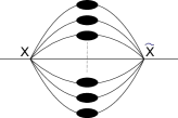
Figure 1: A melon made with $D$ two-point functions with two mirror vertices ${\rm x}$ and $\tilde{\rm x}$.

The first lemma below is already known in the context of ribbon graphs and of colored tensor graphs [6] but not enunciated in the uncolored context (which is the relevant one here).

We start by recalling the definition of tree contraction.

Definition 1.

Given a connected (uncolored) tensor graph ${\mathcal{G}}$ and a tree $T$ of white lines, contracting the tree leads to a reduced graph ${\mathcal{G}}_{1}={\mathcal{G}}/T$ called a (tensor) “rosette”. It has a single vertex which is a $D$-colored tensor graph plus white loop lines and external lines hooked to that vertex.

Lemma 1.

We have, for any connected ${\mathcal{G}}$ and $T$,

$$g_{{\widetilde{J}}}=g_{{\widetilde{J}}_{1}}\,,\qquad g_{J_{\partial}}=g_{{J_{\partial}}_{1}}\,.$$ (2)

Remark 1. We use the obvious notations where the subscript 1 means that the quantities are computed in the tensor rosette graph ${\mathcal{G}}_{1}={\mathcal{G}}/T$. The result therefore holds for any pinched jacket ${\widetilde{J}}$ of $\mathcal{G}_{\text{color}}$ associated with ${\mathcal{G}}$ yielding after contraction the jacket ${\widetilde{J}}_{1}$ of ${\mathcal{G}}_{1}={\mathcal{G}}/T$, and any boundary jacket $J_{\partial}$ of the boundary graph ${\partial\mathcal{G}}$ yielding after contraction the boundary jacket ${J_{\partial}}_{1}$ of the boundary of ${\mathcal{G}}_{1}$.

Proof of Lemma 1. Let $V$ be the number of vertices, $L$ be the number of lines, $F$ the number of faces, and $N_{\text{ext\,}}$ the number of external legs of $\mathcal{G}_{\text{color}}$ extending ${\mathcal{G}}$. We know that $F$ can be decomposed in

$$F=\sum_{k}F_{0k}+\sum_{k}F^{\text{ext\,}}_{0k}+\sum_{kl}F_{kl}\,,$$ (3)

where $0,k,l$ refer to color indices such that $F_{0k}$ denotes the number internal faces of ${\mathcal{G}}$ (of specific pair of colors $0k$), $F_{kl}$ the internal faces of $\mathcal{G}_{\text{color}}$ which does belong to ${\mathcal{G}}$ (the colors $k,l\neq 0$), and $F^{\text{ext\,}}_{0k}$ external (open) faces of ${\mathcal{G}}$.

After a single tree line contraction (note that also this tree line contraction can be referred to as a dipole contraction with two different connected components at the end points of the dipole), we have

$$V\to V-2\,,\qquad L\to L-(D+1)\,,\qquad N_{\text{ext\,}}\to N_{\text{ext\,}}\,,$$ (4)

whereas for faces, one gets the modifications:

$$F_{0k}\to F_{0k}\,,\qquad F_{kl}\to F_{kl}-1\,,\qquad F^{\text{ext\,}}_{0k}\to F^{\text{ext\,}}_{0k}\,.$$ (5)

Let us now consider a jacket ${\widetilde{J}}=(n0m\dots)$ written as a cycle of colors. Some alternating pairs of open faces $F^{\text{ext\,}}_{0n}$ and $F^{\text{ext\,}}_{0m}$ can merge into a single closed face; this happens when they meet white external legs through the “pinching” prescription. The total number of such merged faces is called $\widetilde{F}_{0nm}$ and so, since the jacket ${\widetilde{J}}$ is connected follows from the fact that ${\mathcal{G}}$ is connected and $V_{{\widetilde{J}}}=V$ and $L_{{\widetilde{J}}}=L$,

$$2-2g_{{\widetilde{J}}}=V-L+F_{0n}+F_{0m}+\widetilde{F}_{0nm}+\sum_{kl}F_{kl;\,{\widetilde{J}}}\,,$$ (6)

where the sum over $k,l$ is over $D-1$ (color) pairs in the jacket. Since every term in the sum in $k,l$ changes by $-1$ and $V-L$ by $D-1$, and since $F_{0n}$, $F_{0n}$ and $\widetilde{F}_{0nm}$ have not changed therefore, after contraction,

$$2-2g_{{\widetilde{J}}}\;\to\;2-2g_{{\widetilde{J}}}\quad\Rightarrow\quad g_{{\widetilde{J}}}=g_{{\widetilde{J}}_{1}}\,.$$ (7)

Consider, finally, a boundary jacket $J_{\partial}$ in ${\partial\mathcal{G}}$, $V_{{\partial\mathcal{G}}}=V_{J_{\partial}}=N_{\text{ext\,}}$, $L_{{\partial\mathcal{G}}}=L_{J_{\partial}}=\sum_{k}F^{\text{ext\,}}_{0k}$ are constant. Then, in fact, ${\partial\mathcal{G}}$ is exactly the same. Hence the genus of any boundary jacket $J_{\partial}$ cannot change after contraction. ∎

Remark 2. If every initial vertex of the graph ${\mathcal{G}}$ is a $D$-melon (as is the case for the graphs considered in [1]), then, for any tree $T$, the vertex of rosette ${\mathcal{G}}_{1}$ is again a $D$-melon.

Definition 2.

Given a graph, we define a “closed melopole” as an elementary $D$-dipole made with a 0-line and $D-1$ colored lines (see Fig. 2).

An “open melopole” is defined in the same way but with the 0-line replaced by two open external legs (of course of color 0) (see Fig. 2).

The color of a melopole is the missing color in the dipole defining it (it is also called its“external” color, see “$i$” in Fig. 2).

Figure 2: Closed (left) and open (right) melopole (elementary melon or $D$-dipole containing the color 0) of “external” color i.

Definition 3.

If the single vertex of a rosette is a ($D$) melon graph, we say that the rosette is vertex-melonic.

The melopole contraction of a graph is the recursive contraction of all its closed and open melopoles until none are left.

If the end result of the melopole contraction of a rosette is such that no 0-lines are left, we say that the initial rosette is 0-melonic.

A rosette both vertex and 0-melonic is called fully-melonic.

A melonic line of a vertex-melonic rosette is a line joining two mirror vertices, otherwise it is called non-melonic.

Obviously, a vertex-melonic rosette which is not fully-melonic must have at least one non-melonic line.

Remark 3. The result of the melopole contraction of a graph is independent of the order chosen to perform the recursive contraction of its open and closed melopoles. Given a graph ${\mathcal{G}}$, we denote ${\mathcal{G}}/M$ the graph reduced by the melopole contraction.

In the same previous notations, the following statement holds:

Lemma 2.

The melopole contraction of any graph does not change the genera of its internal and boundary jackets:

$$\forall{\widetilde{J}}\,,\qquad g_{{\widetilde{J}}}=g_{{\widetilde{J}}_{1}}\,,$$ (8)

$$\forall J_{\partial}\,,\qquad g_{J_{\partial}}=g_{{J_{\partial}}_{1}}\,.$$ (9)

Proof. Let us consider first the contraction of a closed melopole of color $i$. We have

$$V\to V-2\,,\qquad L\to L-(D+1)\,,\qquad N_{\text{ext\,}}\to N_{\text{ext\,}}\,.$$ (10)

In the same notations of (3), it can be seen that

$$F_{0k}\to F_{0k}-1\,,\;k\neq i,\qquad F_{0i}\to F_{0i}\,,$$ (11)

$$F_{kl}\to F_{kl}-1\,,\;k,l\neq i,\qquad F_{ki}\to F_{ki}\,,$$ (12)

$$F^{\text{ext\,}}_{0k}\to F^{\text{ext\,}}_{0k}\,,\quad\forall k\,.$$ (13)

Choose a jacket ${\widetilde{J}}=(n0m\dots)$. There are two pairs in the jacket containing $i$ whose face number does not change and so, from (13), $D-1$ remaining change by -1. We infer that $g_{{\widetilde{J}}}$ does not change. Moreover the boundary graph has not changed since $F^{\text{ext\,}}_{0k}\to F^{\text{ext\,}}_{0k}$.

Next, let us consider the case of contraction of an open melopole of color $i$. We note the following:

$$V\to V-2\,,\qquad L\to L-D\,,\qquad N_{\text{ext\,}}\to N_{\text{ext\,}}-2\,,$$ (14)

as well as

$$F_{0k}\to F_{0k}\,,\quad k\neq i\,,\qquad F_{0i}\to F_{0i}\;\;\text{or}\;\;F_{0i}\to F_{0i}+1\,,\qquad$$ (15)

$$F_{kl}\to F_{kl}-1\,,\;k,l\neq i,\qquad F_{ki}\to F_{ki}\,,$$ (16)

$$F^{\text{ext\,}}_{0k}\to F^{\text{ext\,}}_{0k}-1\,.$$ (17)

Let ${\widetilde{J}}=(n0m\dots)$ be a jacket. Two cases might occur:

1. In a first subcase $i\neq n,m$: $D-3$ faces of the type $kl\neq 0i$, jump by -1; $\widetilde{F}_{0nm}$ also jumps by -1. Since $V-L$ varies by $+(D-2)$, then the genus ${\widetilde{J}}$ does not change.

2. In the second subcase $i=n$ (or $i=m$): We have $D-2$ color pairs $kl\neq 0i$ which change by -1; $\widetilde{F}_{0im}$ changes by -1 if and only if $F_{0i}$ jumps by +1. This depends on the fact that the external lines of color $i$ of the dipole belong to a single or to two external open $0i$ faces. In all cases, the genus does not change.

It remains to check the behavior of the boundary graph. The modification here only involves the contraction of a regular melon of a $D$ dimensional color vacuum graph. This is a case completely treated in the colored context (see [6]) and it does not change the genus of any jacket. ∎

The following statement holds:

Lemma 3.

Cutting a white line in a rosette ${\mathcal{G}}$, the quantity $g_{{\widetilde{J}}}$ decreases, for any ${\widetilde{J}}$; the quantity $g_{J_{\partial}}$ increases, for any $J_{\partial}$, and at most by $D$. Hence, in particular, the quantity

$$\sum_{J}g_{{\widetilde{J}}}-k\sum_{J_{\partial}}g_{J_{\partial}}$$ (18)

decreases, for any $k\geq 0$.

Proof. Consider first a jacket ${\widetilde{J}}=(n0m\dots)$. Cutting a white line induces on the number vertices and lines

$$V\to V\,,\qquad L\to L-1\,,$$ (19)

meanwhile for the faces of ${\widetilde{J}}$, $F_{kl}$ do not change (they do not pass by the 0-line cut); there is 1 or 2 faces $F_{0n}$, $F_{0m}$ or $\widetilde{F}_{nm0}$ which pass through the 0-line and they become, respectively, 2 faces or 1 face. Hence,

$$F_{0n}+F_{0m}+\widetilde{F}_{nm0}\to F_{0n}+F_{0m}+\widetilde{F}_{nm0}\pm 1\,.$$ (20)

Thus,

$$g_{{\widetilde{J}}}\to g_{{\widetilde{J}}}\quad\quad\text{or}\quad\quad g_{{\widetilde{J}}}\to g_{{\widetilde{J}}}-1\,.$$ (21)

Let us now consider the boundary graph ${\partial\mathcal{G}}$, with a fixed boundary jacket $J_{\partial}$. Cutting the white line in ${\mathcal{G}}$ changes the boundary ${\partial\mathcal{G}}$ into ${\partial\mathcal{G}}^{\prime}$ (and $J_{\partial}$ to $J_{\partial}^{\prime}$) with two new vertices $V_{1}$ and $V_{2}$ and $D$ new lines of color $1,\dots,D$ which can be partitioned as a disjoint union $S\cup T$, where $S$ is the set of lines joining the two new vertices.

Therefore we have $V_{{\partial\mathcal{G}}^{\prime}}=V_{{\partial\mathcal{G}}}+2\,,\;L_{{\partial\mathcal{G}}^{\prime}}=L_{{\partial\mathcal{G}}}+D$. If we define $\Delta c_{\partial\mathcal{G}}:=c_{{\partial{\mathcal{G}^{\prime}}}}-c_{{\partial\mathcal{G}}}$ (where $c_{{\partial\mathcal{G}}}$ denotes the number of connected components of ${\partial\mathcal{G}}$) and $\Delta F_{J_{\partial}}:=F_{J_{\partial}^{\prime}}-F_{J_{\partial}}$ then

$$g_{J_{\partial}^{\prime}}=g_{J_{\partial}}+\Delta c_{\partial\mathcal{G}}+\frac{D-2-\Delta F_{J_{\partial}}}{2}.$$ (22)

In these notations the fact that $g_{J_{\partial}}$ increases, and by at most $D$, is equivalent to

$$-D-2+2\Delta c_{\partial\mathcal{G}}\leq\Delta F_{J_{\partial}}\leq D-2+2\Delta c_{\partial\mathcal{G}}.$$ (23)

Given a pair of colors $ij$, we have

$$\begin{array}[]{c}F_{ij}\to F_{ij}+1\qquad\text{if}\quad i,j\in S\,,\\ F_{ij}\to F_{ij}\qquad\text{if}\quad i\in S\quad j\in T\quad\text{(or vice-versa)}\,,\\ F_{ij}\to F_{ij}\pm 1\qquad\text{if}\quad i,j\in T\,.\end{array}$$ (27)

The last case can be made more precise: we have $F_{ij}\to F_{ij}-1$ exactly for those pairs $i$ $j$ for which the corresponding lines $i$ and $j$ in the boundary graph belonged to two distinct $ij$ faces.

• If $T=\emptyset$ it is easy to check that $\Delta c_{\partial\mathcal{G}}=1$ and $\Delta F_{J_{\partial}}=D$, hence (23) is true.

• If $S$ and $T$ are both non empty, in the new boundary graph the two new vertices $v_{1}$ and $v_{2}$ belong to a single connected component (because they are necessarily joined by the lines of $S$). This component contains also all other end vertices of the $T$ chains. Observe that if these end vertices belonged to $p$ different connected components in the previous boundary graph, so that $\Delta c_{\partial\mathcal{G}}=1-p$, there has to be also $p$ different components at least in the jacket cycle. Hence, at least $p-1$ pairs $ij$ in the considered jacket with $i\in T$, $j\in T$ which in the initial boundary graph belonged to two distinct $ij$ faces. For them $F_{ij}\to F_{ij}-1$. Furthermore, at least two pairs of the jacket have $i\in S$, $j\in T$. Thus, carefully using (27)

  $$\Delta F_{J_{\partial}}\leq-(p-1)+[D-(2+(p-1))]=D-2p=D-2+2\Delta c_{\partial\mathcal{G}}.$$ (28)

  Moreover again since at least two pairs of the jacket have $i\in S$, $j\in T$, by (27) we have $\Delta F_{J_{\partial}}\geq-D+2$. Since $\Delta c_{\partial\mathcal{G}}-1\leq 0$ this more than implies (23).

  

  Figure 3: Cycle of colors of the jacket. Each color $i$ has two neighbors, $j$ and $j^{\prime}$.

• If $S$ is empty, and the end vertices of the $T$ chains belong again to $p$ different components in ${\partial\mathcal{G}}$, they become either 1 or 2 components in ${\partial{\mathcal{G}^{\prime}}}$ so that $1-p\leq\Delta c_{\partial\mathcal{G}}\leq 2-p$. Since the $p$ different components break the cyclic jacket “circle” (see Figure 3) into at least $p$ different intervals, at least $p$ pairs in the jacket cycle are associated with a change of connected components. For any such pair we must have $F_{ij}\to F_{ij}-1$. Therefore

  $$\Delta F_{J_{\partial}}\leq-p+(D-p)=D-2p\leq D-2+2\Delta c_{\partial\mathcal{G}}.$$ (29)

  Finally in this case $\Delta c_{\partial\mathcal{G}}\leq 1$, and $\Delta F_{J_{\partial}}\geq-D$, hence (23) holds again.

∎

3 Next-to-leading amplitude analysis for a graph

The analysis of the genera of the jackets in a graph with initial melonic vertices, such as those of [1], can be first reduced, through a tree $T$ contraction followed by melonic contraction and using Lemmas 1 and 2 and Remark 2 above, to the analysis of a vertex-melonic rosette without closed or open melopoles. If the initial graph was $D+1$ melonic, that rosette is empty. We carry out now this analysis in the opposite non-trivial case, for which we already remarked that the rosette contains at least one non-melonic white line.

Figure 4: A non-melonic white line (dotted 0-line) joining $x$ and $y\neq\tilde{x}$ yielding a subleading (non-melonic) graph.

Lemma 4.

Let ${\mathcal{G}}$ be a vertex-melonic rosette with a single non-melonic white line $\ell$. We call ${\mathcal{G}}^{\prime}$ the graph in which we cut $\ell$. Then

$$\sum_{J}g_{{\widetilde{J}}}\geq\sum_{J}g_{{\widetilde{J}}^{\prime}}+\frac{D-2}{2}(D-1)!$$ (30)

and moreover

$$\sum_{J}g_{{\widetilde{J}}}-k\sum_{J_{\partial}}g_{J_{\partial}}\geq\sum_{J^{\prime}}g_{{\widetilde{J}}^{\prime}}-k\sum_{J_{\partial}^{\prime}}g_{J_{\partial}^{\prime}}+\frac{D-2}{2}(D-1)!$$ (31)

Proof. Since $\ell$ is non-melonic it joins two vertices $x$ and $y$ such that $y$ is not the mirror vertex $\tilde{x}$ of $x$.

It trivially follows from the Euler relation that, for ribbon graphs, cutting a single line decreases the genus by 0 or 1:

$$V\to V\;,\qquad L\to L-1\,,\qquad F\to F\pm 1\,.$$ (32)

Now coming back to our present situation, $y$ is on a single two-point function of color $i$ joining $x$ to $\tilde{x}$ (see Figure 4). Consider a pair $j,k$ of colors both distinct from $i$ and a jacket ${\widetilde{J}}=(j0k\dots)$. In this jacket, the graph ${\mathcal{G}}^{\prime}$ has two different faces of the $\widetilde{F}_{0jk}$-type, one touching $x$ and the other touching $y$. This is because any path from $x$ to $y$ not using $\ell$ must use color $i$, as seen in Figure 4. Indeed faces of the $\widetilde{F}_{0jk}$-type can use only lines of color j , k or white, and all white lines different from $\ell$ are melonic, hence all those touching the black melon containing $y$ must have their two ends in $y$. Going from ${\mathcal{G}}^{\prime}$ to ${\mathcal{G}}$ closes or merges these two faces in a single one. By the above remark on ribbon graphs, the genus of the jacket ${\widetilde{J}}$ must increase by 1. Repeating the argument for all pairs $j,k$ distinct from $i$ and all jackets of the form $(j0k\dots)$ achieves the proof by a simple counting of all the jackets obtained in this way. Finally (31) is a direct consequence of joining (30) and Lemma 3.

∎

4 Improved power counting for [1]

Let us now specialize to $D=4$, and $k=4$ in Lemmas 3 and 4 and complete the proof of Proposition 1.

Let ${\mathcal{G}}$ be a graph of the theory considered in [1] which satisfies the hypothesis of Proposition 1, hence such that $\sum_{J_{\partial}}g_{J_{\partial}}=q\geq 1$. Its successive reductions (contraction) by an arbitrary tree $T$ of white lines and then by melopoles is called ${\mathcal{G}}_{2}={\mathcal{G}}/(T\cup M)$. According to Lemmas 1 and 2 and since the initial vertices of ${\mathcal{G}}$ were melons, ${\mathcal{G}}_{2}$ is a vertex-melonic rosette. It cannot be fully-melonic (as it would then have trivial melonic boundary) and, by Lemma 3, it has $r\geq q/12$ non-melonic lines, since cutting any non-melonic line moves each $g_{J_{\partial}}$ by at most 4 hence $\sum_{J_{\partial}}g_{J_{\partial}}$, at most, by 12.

Cutting $r-1$ non-melonic lines, one is led to a fully-melonic rosette ${\mathcal{G}}_{3}$ with a single remaining non-melonic line. Applying Lemma 4, we obtain the following:

$$\sum_{J}g_{{\widetilde{J}}}-4\sum_{J_{\partial}}g_{J_{\partial}}=\sum_{J_{2}}g_{{\widetilde{J}}_{2}}-4\sum_{{J_{\partial}}_{2}}g_{{J_{\partial}}_{2}}\geq\sum_{J_{3}}g_{{\widetilde{J}}_{3}}-4\sum_{{J_{\partial}}_{3}}g_{{J_{\partial}}_{3}}\geq 6\,.$$ (33)

The last equality follows from the fact that ${\mathcal{G}}_{4}={\mathcal{G}}_{3}-\ell$ is fully melonic, hence $\sum_{J}g_{{\widetilde{J}}_{4}}-4\sum_{J_{\partial}}g_{{J_{\partial}}_{4}}=0$.

This completes the proof of Proposition 1. ∎

Returning to the list in Section 5 of [1], we remark that inequalities (82) and (85) were used to prove that graphs with $N_{\text{ext\,}}=4$ and $\sum_{J_{\partial}}g_{J_{\partial}}=1$ were convergent. There is a single boundary graph for graphs of this type, namely the one pictured in Fig. 5.

Figure 5: $\phi^{4}$ matrix-like trace invariant interaction.

Interestingly, this term could be interpreted as a $N^{2}$ by $N^{2}$ matrix-like invariant, generating a matrix-like sub-sector of the theory, just like the anomaly term discussed in [1] generates a $N^{4}$ vector-like sector. It might be interesting in fact to construct models in which this subs-ector is divergent, as this may lead to richer models with vector, matrix and tensor aspects at once.

Nevertheless, this is not the case for the model treated in [1]. In that model, graphs with such an external structure converge and do not require any renormalization. Indeed, by Proposition 1 and Equality (42) of [1] (putting $C_{{\partial\mathcal{G}}}=1,V_{4}=0=V_{2}=V_{2}^{\prime\prime}$), their divergence degree is at most $-2$. This concludes our analysis.

References

- [1] J. Ben Geloun and V. Rivasseau, “A Renormalizable 4-Dimensional Tensor Field Theory,” Commun. Math. Phys. 2012, (DOI) 10.1007/s00220-012-1549-1, arXiv:1111.4997 [hep-th].
- [2] V. Rivasseau, “Quantum Gravity and Renormalization: The Tensor Track,” AIP Conf. Proc. 1444, 18 (2011) [arXiv:1112.5104 [hep-th]].
- [3] J. Ben Geloun, “Two and four-loop -functions of rank 4 renormalizable tensor field theories,” arXiv:1205.5513 [hep-th].
- [4] J. Ben Geloun and D. O. Samary, “3D Tensor Field Theory: Renormalization and One-loop -functions,” arXiv:1201.0176 [hep-th].
- [5] V. Bonzom, R. Gurau and V. Rivasseau, “Random tensor models in the large N limit: Uncoloring the colored tensor models,” Phys. Rev. D 85, 084037 (2012) [arXiv:1202.3637 [hep-th]].
- [6] R. Gurau and J. P. Ryan, “Colored Tensor Models - a review,” SIGMA 8, 020 (2012) [arXiv:1109.4812 [hep-th]].
- [7] J. Ben Geloun and E. R. Livine, “Some classes of renormalizable tensor models,” arXiv:1207.0416 [hep-th].
- [8] S. Carrozza, D. Oriti and V. Rivasseau, “Renormalization of Tensorial Group Field Theories: Abelian U(1) Models in Four Dimensions,” arXiv:1207.6734 [hep-th].
- [9] R. Gurau, “The Double Scaling Limit in Arbitrary Dimensions: A Toy Model,” Phys. Rev. D 84, 124051 (2011) [arXiv:1110.2460 [hep-th]].
- [10] R. Gurau, “Universality for Random Tensors,” arXiv:1111.0519 [math.PR].
- [11] V. Bonzom, R. Gurau, A. Riello and V. Rivasseau, “Critical behavior of colored tensor models in the large N limit,” Nucl. Phys. B 853, 174 (2011) [arXiv:1105.3122 [hep-th]].
- [12] R. Gurau, “The complete 1/N expansion of colored tensor models in arbitrary dimension,” Annales Henri Poincare 13, 399 (2012) [arXiv:1102.5759 [gr-qc]].