Antiscreening in perturbative quantum gravity and resolving the Newtonian singularity

Abstract

We calculate the quantum corrections to the Newtonian potential induced by a massless, nonminimally coupled scalar field on Minkowski background. We make use of the graviton vacuum polarization calculated in our previous work and solve the equation of motion nonperturbatively. When written as the quantum-corrected gauge invariant Bardeen potentials, our results show that quantum effects generically antiscreen the Newtonian singularity $\propto 1/r$. This result supports the point of view that gravity on (super-)Planckian scales is an asymptotically safe theory. In addition, we show that, in the presence of quantum fluctuations of a massless, (non)minimally coupled scalar field, dynamical gravitons propagate superluminally. The effect is, however, unobservably small and it is hence of academic interest only.

I Introduction

In Ref. Marunovic:2011zw we considered the graviton vacuum polarization induced by the one-loop quantum fluctuations of a nonminimally coupled, massless scalar field on Minkowski background in the Schwinger-Keldysh formalism. This allowed us to compute the large distance, leading order, quantum correction to the scalar gravitational (Bardeen) potentials, which in longitudinal gauge reduce to the Newtonian potentials. We used the Schwinger-Keldysh formalism in direct (coordinate) space which allowed us to study time transients associated with switching on scalar vacuum fluctuations at a definite moment in time. Such transients can be induced, for example, by symmetry restoration that renders the scalar field massless. Moreover, just as in the presence of classical matter, the two quantum Bardeen potentials differ when the effects of quantum (scalar) matter fluctuations are included.

In Ref. Marunovic:2011zw we adopted the effective approach to quantum gravity (see e.g. Refs. Donoghue:1994A ; Donoghue:1994B ), according to which quantum gravitational effects can be reliably calculated by perturbative methods, provided one focuses on low energy and momentum phenomena. By now, there is quite a long history and extensive literature on long range, quantum corrections to the Newtonian potentials. Such studies were pioneered by Donoghue Donoghue:1994A ; Donoghue:1994B , and followed by many others HamberLiu:1995 ; Akhundov:1997 , with differing results. The problem was again revived in the 2000s in Refs. BjerrumBohr:2002A ; BjerrumBohr:2002B ; BjerrumBohr:2003C ; Butt:2006 ; Faller:2008 ; Dalvit:1994gf ; Satz:2004hf , where also some of the graviton vertex corrections were included. The Schwinger-Keldysh formalism was for the first time used in Ref. Park:2011ww . Related older works include Capper:1979ej ; Capper:1978yf where the one-loop graviton vacuum polarization induced by photons on a Minkowski background was calculated.

Here we extend our work in Marunovic:2011zw and present a resummation scheme by which we consider short and large scale screening effects of gravitational potentials induced by quantum fluctuations of a massless nonminimally coupled scalar. More precisely, we make use of the one-particle irreducible (1PI) resummation technique and arrive at the result that the Newtonian potentials exhibit a strong antiscreening at length scales of the order of the Planck scale. Surprisingly, there are also long range oscillatory quantum corrections to the Newtonian potentials. Even though these corrections are present at large distances, they are high energy corrections, since oscillations occur at the Planck length scale.

Admittedly, these results do not belong to the realm of effective quantum gravity, questioning their reliability. Still, we feel compelled to present them, and believe that they deserve some attention. Indeed, this work is not the first attempt to use a resummation technique to investigate short scale effects in quantum gravity. The main other contender is known as the effective action approach to quantum gravity Reuter:1996cp , and it is usually implemented within the asymptotic safety program for quantum gravity, and we shall now recall the basic idea behind this approach.

The asymptotic safety program in quantum gravity was initiated by Weinberg Hawking:1979ig , where he argued that a weaker requirement than the usual renormalizability may be imposed on quantum gravity. Recently, this program has attracted a considerable attention among researchers in quantum gravity Reuter:2012id ; Niedermaier:2006ns . If quantum gravity were an asymptotically safe theory, it would exhibit few-dimensional critical hypersurface characterizing the running of relevant couplings (that are associated with relevant operators). The running of these couplings ”emanate” from an ultraviolet (UV) fixed point, at which their value has a definite value that can be, in principle, determined. The claim is that the set of relevant operators consists of unity (the corresponding coupling being the cosmological term), the Ricci scalar (the corresponding coupling being the Newton constant) and possibly some quadratic curvature invariants. There is limited evidence that all other (higher derivative) operators are irrelevant, in the sense that the UV fixed point ”repels” the corresponding couplings as one runs towards the ultraviolet. The value of these irrelevant couplings is (at least in principle) uniquely determined by the requirement that the physical theory runs towards the UV fixed point, as the running scale approaches infinity. Thus, an asymptotically safe quantum gravity consists of several (relevant) couplings whose value ought to be determined by measurements, for example in the far infrared, while all other coupling parameters are given by the requirement of asymptotic safety. Within this framework it is not true anymore that there are infinitely many counterterms appearing in perturbation theory, whose coefficients (couplings) must be determined by (an infinite number of) measurements. In this sense the asymptotic safety program resolves the problem of nonrenormalizability of quantum gravity. What remains to be shown is that quantum gravity is indeed an asymptotically safe theory, which is far from a trivial pursuit.

Indeed, the proof that quantum gravity is asymptotically safe would require solving quantum gravity nonperturbatively, which is very hard. Instead, researchers have focused on developing perturbative and nonperturbative methods (for reviews, see Reuter:2012id ; Niedermaier:2006ns ), hoping to collect enough evidence in support of the asymptotic safety hypothesis. The original evidence due to Weinberg Hawking:1979ig is based on an $\epsilon$-expansion around two spacetime dimensions. Here, $\epsilon=2$ is not a small number in four spacetime dimensions, making the whole approach questionable. The second approach is based on a functional renormalization group equation for the gravitational effective action pioneered by Reuter Reuter:1996cp . While the starting equation is an exact (functional) differential equation for the effective gravitational action, the actual approximation scheme is limited to an a priori chosen set of local operators, truncated at some order (usually fourth) in space and time derivatives. The criticism of the method is twofold. Firstly, the operators are chosen a priori based on a derivative expansion which is essentially a low energy expansion, while the application is extended to the ultraviolet sector. Secondly, the operators of canonical dimension four or higher generically violate unitarity, questioning thus the validity of the whole (nonperturbative) scheme. Yet, the results (if true) are fascinating: they suggest existence of an ultraviolet (UV) non-Gaussian, nontrivial, fixed point in quantum gravity. Close to this UV fixed point the Newton constant runs with a scale $\mu$ as $G_{N}(\mu)\simeq g_{*}/\mu^{2}$ (as $\mu\rightarrow\infty$) , while the cosmological constant runs as $\Lambda(\mu)\simeq\lambda_{*}\mu^{2}$, where $g_{*}\simeq 0.27$ and $\lambda_{*}\simeq 0.35$ are calculable (nonvanishing) real constants. While the traditional approach to asymptotic safety is to demand that one obtains the Einstein-Hilbert action in the deep infrared, recently Satz et at. Satz:2010uu have developed an effective average action approach starting in the infrared with the Barvinsky-Vilkovisky non-local effective action Barvinsky:1987uw ; Barvinsky:1990up , which takes account of one-loop massless field excitations of fields with various spins.

In this work we present a different resummation scheme, such that antiscreening occurs as a result of resumming the one-loop 1PI diagrams for the gravitational potentials. In contrast to the local operator approach mentioned above, where a derivative expansion is used, our resummation is based on a nonlocal correction to the graviton vacuum polarization, and thus does not suffer from the above problems. The hope is that, if we choose the coefficients of the finite counterterms to be zero, our method will not violate unitarity. Furthermore, our method does not violate any of the symmetries of the theory. Namely, we linearize in the gravitational field, and in our analysis we maintain the linear version of diffeomorphism invariance (also known as gauge invariance).

The paper is organized as follows: in Sec. II we present a self-consistent solution to the one-loop 1PI effective field equations for the gravitational potentials. In Sec. III we discuss our results and give an outlook for future work.

Unless stated explicitly, we work in natural units where $\hbar=1=c$.

II Resummation

The quantum corrected equation of motion for the linearized Einstein equation (see Eq. (39) in Marunovic:2011zw ) is of the form

$$L_{\mu\nu\rho\sigma}h^{\rho\sigma}(x)+\int d^{4}x^{\prime}\left[{}_{\mu\nu}\Pi_{\rho\sigma}^{\rm ret}\right](x;x^{\prime})h^{\rho\sigma}(x^{\prime})+{\cal O}((h_{\mu\nu})^{2})=\frac{\kappa^{2}}{2}\delta_{\mu}^{0}\delta_{\nu}^{0}M\delta^{3}(\vec{x}),$$ (1)

where $\left[{}_{\mu\nu}\Pi_{\rho\sigma}^{\rm ret}\right](x;x^{\prime})$ is the retarded graviton vacuum polarization tensor of the graviton field perturbation $h_{\mu\nu}(t,\vec{r}\,)$, $M$ is a (static) particle’s mass and $\kappa^{2}=16\pi G_{N}$; $G_{N}$ is Newton’s constant. A massless, nonminimally coupled scalar field on Minkowski background induces at one-loop the following renormalized graviton vacuum polarization tensor:

$$\left[{}_{\mu\nu}\Pi_{\rho\sigma}^{\rm ret}\right](x;x^{\prime}) = -\frac{\kappa^{2}}{7680\pi^{3}}\times L_{\mu\nu\alpha\beta}\bigg{\{}D^{\alpha\beta}{}_{\rho\sigma}-\eta^{\alpha\beta}D_{\rho\sigma}\bigg{[}\frac{1}{6}+30\Big{(}\xi-\frac{1}{6}\Big{)}^{2}\bigg{]}\bigg{\}}$$ (2)

$$\hskip 39.83368pt\times\,\partial^{4}\,\Theta(\Delta t^{2}-\Delta r^{2})\Theta(\Delta t)\left[\ln|\mu^{2}(\Delta r^{2}-\Delta t^{2})|-1\right]\,,$$

where $\Delta r=\|\vec{x}-\vec{x}^{\,\prime}\|$, $\Delta t=t-t^{\prime}$ ($\vec{x}$, $\vec{x}^{\,\prime}$, $t$ and $t^{\prime}$ denote spatial and time coordinates, respectively), $\xi$ measures the coupling strength of the scalar filed $\varphi$ to gravity through the Ricci scalar $R$,  and $L_{\mu\nu\rho\sigma}$ denotes the Lichnerowicz operator on Minkowski background:

$$L_{\mu\nu\rho\sigma}=D_{\mu\nu\rho\sigma}-\frac{1}{2}\eta_{\mu\nu}D_{\rho\sigma}\,,$$ (3)

with the explicit form of the operators,

$$D_{\rho\sigma}=\partial_{\rho}\partial_{\sigma}-\eta_{\rho\sigma}\partial^{2}\;,\qquad D_{\mu\nu\rho\sigma}=\partial_{(\rho}\eta_{\sigma)(\mu}\partial_{\nu)}-\frac{1}{2}\eta_{\mu(\rho}\eta_{\sigma)\nu}\partial^{2}-\frac{1}{2}\eta_{\rho\sigma}\partial_{\mu}\partial_{\nu}\,,$$ (4)

$\partial^{2}=\eta^{\gamma\delta}\partial_{\gamma}\partial_{\delta}$ and indices in (1) are lifted with the Minkowski metric, $\eta^{\mu\nu}={\rm diag}(-1,1,1,1)$. Analogous results were found earlier in Horowitz:1980fj ; Jordan:1987wd , albeit the equation of motion was presented in a form somewhat different from (1) and (2).

In this paper we solve the 1PI equation of motion for the graviton one-point function (1) exactly. This corresponds to resumming all 1PI one-loop diagrams, illustrated in Fig. 1, where we show the nonlocal contribution arising from cubic graviton-scalar vertices, the local contribution from quartic scalar-graviton vertices, and the counterterm contribution. In order to illustrate how the resummation works, in Fig. 2 we show the resummed nonlocal diagrams (arising from cubic vertices). In principle, the contribution from the local diagrams needs to be resummed as well. But, in a flat spacetime background they contribute only as power-law divergences, their contribution gets automatically subtracted in dimensional regularization, and thus they do not contribute Marunovic:2011zw .

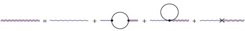
Figure 1: The resummed one-loop contribution from scalar vacuum fluctuations to the graviton propagator.

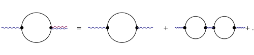
Figure 2: The resummed contribution from the nonlocal (cubic) vertices to the graviton propagator. The resummed loop can be written as a sum of the one-loop, two-loop, etc., contributions.

To proceed, note first that it helps to insert instead of the source on the right-hand side of (1) the classical equation of motion

$$L_{\mu\nu\rho\sigma}h^{\rho\sigma(c)}(x)=\;\frac{\kappa^{2}}{2}\;\delta_{\mu}^{0}\delta_{\nu}^{0}M\delta^{D-1}(\vec{x}),$$ (5)

where superscript $c$ stands for classical. This enables us to completely remove the Lichnerowicz operator from Eq. (1) and thus relate the quantum gravitational field to the classical potential through an integral equation:

$$h^{\alpha\beta(c)}(x) = h^{\alpha\beta}(x)-\frac{\kappa^{2}}{7680\pi^{3}}\bigg{\{}D^{\alpha\beta}{}_{\rho\sigma}-\eta^{\alpha\beta}D_{\rho\sigma}\bigg{[}\frac{1}{6}+30\Big{(}\xi-\frac{1}{6}\Big{)}^{2}\bigg{]}\bigg{\}}$$ (6)

$$\times\partial^{4}\int d^{4}x^{\prime}\Theta(\Delta t^{2}-\Delta r^{2})\Theta(\Delta t)\left[\ln(\mu^{2}(\Delta t^{2}-\Delta r^{2}))-1\right]h^{\rho\sigma}(x^{\prime}).$$

This form of the equation suggests that the vacuum polarization can be thought of as a (nonlocal, spacetime dependent, causal) wave function renormalization of the graviton $h^{\alpha\beta}(x)$. In the Appendix we show how to solve this equation. The general solutions in momentum space are given in Eqs. (68) and (69). Here we are interested in a static response to a point mass, for which the classical Bardeen potentials in momentum space are $\Phi^{(c)}=\Psi^{(c)}=-[4\pi G_{N}M/k^{2}]\times 2\pi\delta(k^{0})$, $k\equiv\|\vec{k}\|$ (see Ref. Marunovic:2011zw ). Hence, a static response to a point mass $M$ is obtained simply by taking the limit $k^{0}\rightarrow 0$ of Eqs. (68) and (69):

$$\Phi(k^{\mu}) = -\frac{4\pi G_{N}M\times 2\pi\delta(k^{0})}{k^{2}}\Bigg{[}\frac{4}{3}\frac{1}{1+k^{2}{\cal K}}-\frac{1}{3}\frac{1}{1-5(1-6\xi)^{2}k^{2}{\cal K}}\Bigg{]}\,,\qquad$$ (7)

$$\Psi(k^{\mu}) = -\frac{4\pi G_{N}M\times 2\pi\delta(k^{0})}{k^{2}}\Bigg{[}\frac{1}{3}\frac{1}{1+k^{2}{\cal K}}+\frac{2}{3}\frac{1}{1-5(1-6\xi)^{2}k^{2}{\cal K}}\Bigg{]}\,,$$ (8)

where, in the static limit,

$$k^{2}{\cal K}=\frac{G_{N}k^{2}}{60\pi}\Big{[}\ln\Big{(}\frac{k}{2\mu}\Big{)}+\gamma_{E}\Big{]}\,.$$ (9)

Since for the vector and tensor perturbations classical fields vanish, Eqs. (62) and (63) imply that, at one-loop order, also the quantum corrected fields vanish, $\tilde{n}^{T}_{i}=0=h_{ij}^{TT}$.

Upon performing an inverse Fourier transformation and setting $x\equiv kl_{Pl}$, $\tilde{\mu}\equiv\mu l_{Pl}{\rm e}^{-\gamma_{E}}$, $y\equiv r/l_{Pl}$ (where $l_{Pl}=\sqrt{G_{N}}$ is the Planck length), we arrive at the solution for the gauge invariant scalars in position space:

$$\Phi(r) = -\frac{2G_{N}M}{\pi r}\int_{0}^{\infty}\frac{dx\sin(xy)}{x}\left\{\frac{4}{3}\frac{1}{1+\frac{x^{2}}{120\pi}\ln\left(\frac{x^{2}}{4\tilde{\mu}^{2}}\right)}-\frac{1}{3}\frac{1}{1-(1-6\xi)^{2}\frac{x^{2}}{24\pi}\ln\left(\frac{x^{2}}{4\tilde{\mu}^{2}}\right)}\right\}\,,$$ (10)

$$\Psi(r) = -\frac{2G_{N}M}{\pi r}\int_{0}^{\infty}\frac{dx\sin(xy)}{x}\left\{\frac{2}{3}\frac{1}{1+\frac{x^{2}}{120\pi}\ln\left(\frac{x^{2}}{4\tilde{\mu}^{2}}\right)}+\frac{1}{3}\frac{1}{1-(1-6\xi)^{2}\frac{x^{2}}{24\pi}\ln\left(\frac{x^{2}}{4\tilde{\mu}^{2}}\right)}\right\}\,.$$ (11)

As such these integrals cannot be computed analytically. However, it is feasible to examine their behavior for small $r$ and for large $r$.

For small $r$ and for nonconformal coupling ($\xi\neq 1/6$) both integrals are proportional to $r$ with the constant of proportionality depending on the coupling strength $\xi$ only. This is the main result of this section as it clearly shows that the $1/r$ singularity is screened on Planck scales by quantum effects (see Figs. 3 and 4 for $r_{S}/l_{Pl}=10$ and Figs. 5 and 6 for $r_{S}/l_{Pl}=0.05$, where $r_{S}=2G_{N}M$ is the Schwarzschild radius). Nevertheless, in the case of the conformal coupling ($\xi=1/6$) the second integral in the above expressions reduces to a constant while the first one is proportional to $r$. This means that for the conformal coupling there is no screening of the Newtonian singularity (in this case quantum effects do not increase the order of singularity at the origin), which means that quantum effects are the weakest in the conformally coupled case.

For large $r$, the first integral, denoted by $I_{1}(y)$

$$I_{1}(y)=\int_{0}^{\infty}\frac{dx\sin(xy)}{x}\frac{1}{1+\frac{x^{2}}{120\pi}\ln\left(\frac{x^{2}}{4\tilde{\mu}^{2}}\,{\rm e}^{2\gamma_{E}}\right)},$$ (12)

is rather simple and yields a constant $I_{1}(y)={\pi}/{2}$, while the second one, we denote by $I_{2}(y)$,

$$I_{2}(y)=\int_{0}^{\infty}\frac{\sin(xy)dx}{x}\frac{1}{1-(1-6\xi)^{2}\frac{x^{2}}{24\pi}\ln\left(\frac{x^{2}}{4\tilde{\mu}^{2}}\,{\rm e}^{2\gamma_{E}}\right)}$$ (13)

is more delicate and needs to be treated heedfully. As $\xi\neq 1/6$, the denominator in this integral has poles on the real axis denoted as $\pm x_{c}$. In order to calculate the principal part of the integral, we approximate the log-function by a constant evaluated at $x_{c}$. This is justified by the fact that the log-function is the largest (but finite) at the pole. In this approximation the integral becomes

$$I_{2}(y)=-\frac{1}{2}\int_{0}^{\infty}dx\sin(xy)\left(\frac{1}{x-x_{c}}+\frac{1}{x+x_{c}}-\frac{2}{x}\right)\,,$$ (14)

where $x_{c}=x_{c}(\xi,\mu)$ is the (positive, real) solution of the transcendental equation

$$x_{c}^{2}\times\frac{(1-6\xi)^{2}}{24\pi}\ln\left(\frac{x_{c}^{2}}{4\tilde{\mu}^{2}}\,{\rm e}^{2\gamma_{E}}\right)=1\,.$$ (15)

The approximate integral (14) can be expressed in terms of the sine integral $\mbox{Si}(x)$ and the cosine integral $\mbox{Ci}(x)$, defined by

$$\mbox{Si}(x)=-\int_{x}^{\infty}\frac{\sin(z)dz}{z}\,,\qquad\mbox{Ci}(x)=-\int_{x}^{\infty}\frac{\cos(z)dz}{z}\,.$$ (16)

Using asymptotic expansions of $\mbox{Si}(x)$ and $\mbox{Ci}(x)$, we get the following approximate expression for $I_{2}$ in the limit of large $r$:

$$I_{2}(y)\approx\frac{\pi}{2}\left[1-\cos(x_{c}y)\right]\,.$$

This result needs to be checked against the numerical one. It turns out that one gets agreement, provided one modifies the coefficient in front of the cosine function by a function $a(\xi)$ that weakly depends on $\xi$. So a better approximation for asymptotically large $r$ is

$$I_{2}(y)=\frac{\pi}{2}\left[1-a(\xi)\cos(x_{c}y)\right]\,,$$ (17)

where $a(\xi)\sim 1$. When this and $I_{1}=\pi/2$ are inserted into (10–11) one arrives at the following asymptotic form for the Bardeen potentials:

$$\Phi = -\frac{G_{N}M}{r}\bigg{\{}1+\frac{1}{3}a(\xi)\cos(\kappa_{c}r)\bigg{\}}$$ (18)

$$\Psi = -\frac{G_{N}M}{r}\bigg{\{}1-\frac{1}{3}a(\xi)\cos(\kappa_{c}r)\bigg{\}}\,,$$ (19)

where $yx_{c}=\kappa_{c}r$, $\kappa_{c}=x_{c}/l_{Pl}$. Notice that, unlike in the classical case, the one-loop scalar quantum fluctuations generate different Bardeen potentials at large $r$. The Bardeen potentials exhibit oscillatory behavior at large $r$. These oscillations occur at the Planck scale, and their amplitude is about 1/3 of the classical potential (modulated by a weakly dependent function of $\xi$ of order 1). When the effective action of Ref Satz:2010uu is used to calculate quantum corrections to the Newtonian potential, apart from the usual $\propto 1/r^{3}$ term, the authors of Satz:2010uu obtained oscillatory terms $\propto\sin(\mu r)/r^{5/2}$, where $\mu$ is the renormalization scale. It would be of interest to find out if there is a relation to the oscillatory terms found in this work. Equations (18) and (19) comprise the second main result of this work.

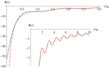
Figure 3: The quantum corrected Bardeen potential $\Phi$, obtained numerically, is represented by the solid line; the long-dashed line represents its analytical expression (18) for large $r$ behavior; the short-dashed line shows Newtonian potential. Values of the parameters are $\xi=0$ (or $\xi=1/3$), $\tilde{\mu}=1$ and $r_{S}/l_{Pl}=10$.

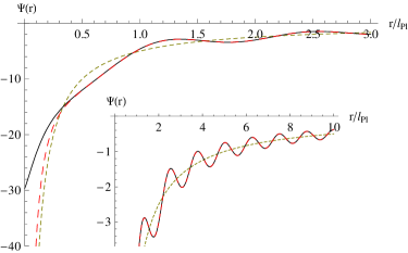
Figure 4: The quantum corrected Bardeen potential $\Psi$, obtained numerically, is represented by the solid line; the long-dashed line represents its analytical expression (19) for large $r$ behavior; the short-dashed line shows Newtonian potential. Values of the parameters are $\xi=0$ (or $\xi=1/3$), $\tilde{\mu}=1$ and $r_{S}/l_{Pl}=10$.

In Figs. 3 – 6 we show the numerically evaluated quantum corrected Bardeen potentials as a function of the distance from the point mass $M$. While Figs. 3 and 4 show the Bardeen potentials for a heavy mass, $M\gg m_{Pl}$, Figs. 5 and 6 show the Bardeen potentials induced by a light mass, $M\ll m_{Pl}$ (which holds for the mass of all known elementary particles). The Figs. show that, when quantum fluctuations are included (solid lines), the Newtonian potentials (short-dashed lines) get antiscreened such that the Newtonian singularity $\propto 1/r$ gets resolved. Furthermore, for large $r$, there is very good agreement between our semianalytical expressions for the Bardeen potentials (18) and (19) and the curves obtained by numerical integration. Next, we show how the potentials depend on the $r_{S}/l_{Pl}$ parameter. In general, if the Schwarzschild radius is greater than the Planck length then an event horizon forms (a property characterizing black holes), in which case the Bardeen potential $\Psi$ crosses $-1/2$. This is exactly what we see in Fig. 4. However, if the Schwarzschild radius is less than the Planck length (as it is the case with all known elementary particles) then no event horizon forms, i.e. $\Psi>-1/2$ for all $r$. This feature is clearly manifested in Figs. 5 and 6.

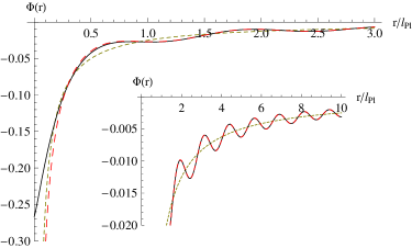
Figure 5: The quantum corrected Bardeen potential $\Phi$, obtained numerically, is represented by the solid line; the long-dashed line represents its analytical expression (18) for large $r$ behavior; the short-dashed line shows Newtonian potential. Values of the parameters are $\xi=0$ (or $\xi=1/3$), $\tilde{\mu}=1$ and $r_{S}/l_{Pl}=0.05$.

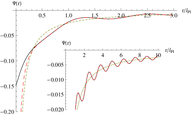
Figure 6: The quantum corrected Bardeen potential $\Psi$, obtained numerically, is represented by the solid line; the long-dashed line represents its analytical expression (19) for large $r$ behavior; the short-dashed line shows Newtonian potential. Values of the parameters are $\xi=0$ (or $\xi=1/3$), $\tilde{\mu}=1$ and $r_{S}/l_{Pl}=0.05$.

We have seen that quantum fluctuations antiscreen gravitational potentials in the sense that they reach a finite value when $r\rightarrow 0$. For small $r$ the potentials are linear in $r$, i.e. $\Phi\simeq\Phi_{0}+\Phi_{0}^{\prime}r$, $\Psi\simeq\Psi_{0}+\Psi_{0}^{\prime}r$. The resulting gravitational force, $\vec{F}=-\nabla\Phi=-\Phi_{0}^{\prime}\vec{r}/r$ is constant and negative, implying that the force reaches a maximum amount. This is to be contrasted with the Newton force, which grows without a limit as $\propto 1/r^{2}$ at small $r$. Let us now consider the Riemann curvature tensor $R_{\rho\sigma\mu\nu}$. When linearized in $h_{\mu\nu}$,

$$R_{\rho\sigma\mu\nu}=\partial_{\mu}\Big{[}\partial_{(\nu}h_{\sigma)\rho}-\frac{1}{2}\partial_{\rho}h_{\nu\sigma}\Big{]}-\partial_{\nu}\Big{[}\partial_{(\mu}h_{\sigma)\rho}-\frac{1}{2}\partial_{\rho}h_{\mu\sigma}\Big{]}\,.$$ (20)

Taking account of symmetries of the Riemann tensor, the nonvanishing components of (20) can be written in terms of gauge invariant components of $h_{\mu\nu}$ only as

$$R_{0i0j} = -R_{i00j}=-R_{i00j}=R_{i0j0}=R_{j0i0}=\partial_{i}\partial_{j}\Phi+\delta_{ij}\partial_{0}^{2}\Psi+\partial_{0}\partial_{(i}\tilde{n}_{j)}^{T}-\frac{1}{2}\partial_{0}^{2}h_{ij}^{TT}\,,$$

$$R_{0ijl} = -R_{i0jl}=R_{jl0i}=-R_{jli0}=2\partial_{0}\partial_{[j}\delta_{l]i}\Psi-\partial_{0}\partial_{[j}h_{l]i}^{TT}\,,$$

$$R_{ijkl} = -R_{jikl}=-R_{ijlk}=R_{klij}=4\partial_{[i}\delta_{j][k}\partial_{l]}\Psi+\big{(}\partial_{j}\partial_{[k}h_{l]i}^{TT}-\partial_{i}\partial_{[k}h_{l]j}^{TT}\big{)}\,.$$ (21)

When applied to the problem at hand ($h_{ij}^{TT}=0$, $\partial_{0}\Psi=0$, $\tilde{n}_{i}^{T}=0$), these reduce to

$$R_{0i0j} = \Big{(}\frac{\delta_{ij}}{r}-\frac{x_{i}x_{j}}{r^{3}}\Big{)}\Phi_{0}^{\prime}\,,\qquad R_{0ijl}=0\,,$$

$$R_{ijkl} = 4\Big{(}\frac{\delta_{j[k}\delta_{l]i}}{r}-\frac{x_{[i}\delta_{j][k}x_{l]}}{r^{3}}\Big{)}\Psi_{0}^{\prime}\,,$$ (22)

from which we can obtain the Ricci curvature tensor and scalar,

$$R_{00}=\frac{2}{r}\Phi_{0}^{\prime}\,,\qquad R_{ij}=-\Big{(}\frac{\delta_{ij}}{r}-\frac{x_{i}x_{j}}{r^{3}}\Big{)}\Phi_{0}^{\prime}-\Big{(}\frac{3\delta_{ij}}{r}-\frac{x_{i}x_{j}}{r^{3}}\Big{)}\Psi_{0}^{\prime}\,,\qquad R=-\frac{4}{r}\Phi_{0}^{\prime}-\frac{8}{r}\Psi_{0}^{\prime}\,.$$ (23)

From these equations we see that a curvature singularity remains. It is however reduced from the standard curvature singularity of a black hole, $R_{\rho\sigma\mu\nu}R^{\rho\sigma\mu\nu}=(48G_{N}^{2}M^{2})/r^{6}$ (which is present only in the Weyl part of the Riemann tensor since $R_{\mu\nu}=0$) to much milder curvature-squared singularities,

$$R_{\mu\nu}R^{\mu\nu}=\frac{2}{r^{2}}(3{\Phi_{0}^{\prime}}^{2}+6\Psi_{0}^{\prime}\Phi_{0}^{\prime}+11{\Psi_{0}^{\prime}}^{2})\,,\qquad R_{\rho\sigma\mu\nu}R^{\rho\sigma\mu\nu}=\frac{8}{r^{2}}(\Phi_{0}^{\prime\,2}+3\Psi_{0}^{\prime\,2})\,,$$ (24)

which for small $r$ are of the order $\sim 1/r^{2}$. It would be of interest to check whether this behavior persists at two-loop order, or perhaps the screening of gravitational potentials is more efficient when higher loop effects are taken into account. Such an analysis would increase our understanding of the strength of gravity at very small (Planckian) scales.

III Quantum gravitational radiation

Here we discuss how the one-loop vacuum polarization from (nonminimally coupled massless) scalars (2) affects the propagation of gravitational waves. For simplicity, we perform here a perturbative analysis of the 1PI resummed equation (63), and we shall work in direct space. This section is inspired by the recent paper of Leonard and Woodard Leonard:2012fs , where it was shown that the photon one-loop vacuum polarization induced by the graviton vacuum fluctuations affects propagation of the photons by deforming its light cone. Here we shall see that the analogous effect is present in the case of dynamical gravitons immersed in a sea of vacuum fluctuations of matter fields.

We begin our analysis by a simple quadrupole model, for which nonvanishing components of the conserved energy momentum tensor are

$$T_{00}(\vec{x},t) = \tilde{I}_{ij}r(t)\partial_{i}\partial_{j}\delta^{3}(\vec{x})$$

$$T_{0i}(\vec{x},t) = \tilde{I}_{ij}\Theta(t)\partial_{j}\delta^{3}(\vec{x})$$

$$T_{ij}(\vec{x},t) = \tilde{I}_{ij}\delta(t)\delta^{3}(\vec{x})\,,$$ (25)

where $\tilde{I}_{ij}=\int d^{4}x{\rm e}^{\imath k\cdot x}T_{ij}(x)$ is the transverse, traceless, momentum space moment of inertia, satisfying $\tilde{I}_{ii}=0$ and $\partial_{i}\tilde{I}_{ij}=0$ and $r(t)$ is a ”ramp” function $dr(t)/dt=\Theta(t)$, and $d\Theta(t)/dt=\delta(t)$. Of course, the stress energy tensor (25) is an approximation to a realistic explosive event with a nonvanishing quadrupole, which has a finite spatial extension. The classical, gauge invariant equation for the (transverse-traceless) graviton is

$$\partial^{2}h_{ij}^{(c)TT}(x)=-16\pi G_{N}T_{ij}\,$$ (26)

and its solution for the stress energy tensor (25) is the Einstein quadrupole formula,

$$h_{ij}^{(c)TT}(x)=4G_{N}\tilde{I}_{ij}\frac{\delta(t-r)}{r}=8G_{N}\tilde{I}_{ij}\Theta(t)\delta(x^{2})\,,\qquad x^{2}=-t^{2}+r^{2},\quad r\equiv\|\vec{x}\|\,.$$ (27)

An inspection of Eq. (63) shows that, at this order, quantum effects do not mix tensor perturbations with scalar or vector perturbations. Thus, Eqs. (40) and (41) can be rewritten for $h_{ij}^{TT}$ as

$$h^{(c)TT}_{ij}(x)=h^{TT}_{ij}(x)-\frac{\kappa^{2}}{7680\pi^{3}}\bigg{\{}D_{ijkl}-\delta_{ij}D_{kl}\bigg{[}\frac{1}{6}+30\Big{(}\xi-\frac{1}{6}\Big{)}^{2}\bigg{]}\bigg{\}}F_{kl}(x)\,,$$ (28)

where

$$F_{kl}(x)=\partial^{2}\int d^{4}x^{\prime}\Theta(\Delta t^{2}-\Delta r^{2})\Theta(\Delta t)\left[\ln(\mu^{2}(\Delta t^{2}-\Delta r^{2}))-1\right]{\partial^{\prime}}^{2}h_{kl}^{TT}(x^{\prime})\,,$$ (29)

where we have moved by partial integration two out of four derivatives to act on $h_{kl}^{TT}$. Equations (28) and (29) can be solved perturbatively, by writing $h_{kl}^{TT}=h_{kl}^{(c)TT}+h_{kl}^{(q)TT}$, where $h_{kl}^{(c)TT}$ is the classical solution (27) and $h_{kl}^{(q)TT}$ is the quantum correction. Inserting this into (28) and (29) results in

$$h^{(q)TT}_{ij}(x)=\frac{G_{N}}{480\pi^{2}}\bigg{\{}D_{ijkl}-\delta_{ij}D_{kl}\bigg{[}\frac{1}{6}+30\Big{(}\xi-\frac{1}{6}\Big{)}^{2}\bigg{]}\bigg{\}}F_{kl}(x)\,.$$ (30)

Inserting $h_{kl}^{(c)TT}$ into (29) yields the leading order (one-loop) quantum correction to the graviton field. Making use of (26), Eq. (29) simplifies to

$$F_{kl}(x)=-16\pi G_{N}\tilde{I}_{ij}\partial^{2}\left\{\Theta(t^{2}-r^{2})\Theta(t)\left[\ln(\mu^{2}(t^{2}-r^{2}))-1\right]\right\}\,.$$ (31)

Acting naively with the last two derivatives is problematic as it leads to singular expressions. This can be resolved by recalling that in the Schwinger-Keldysh formalism the retarded vacuum polarization originates from

$$F_{kl}(x) = -16\pi G_{N}\tilde{I}_{ij}\partial^{2}\left\{\frac{\left[\ln^{2}(\mu^{2}x^{2}_{++})-2\ln(\mu^{2}x^{2}_{++})\right]-\left[\ln^{2}(\mu^{2}x^{2}_{+-})-2\ln(\mu^{2}x^{2}_{+-})\right]}{4\pi\imath}\right\}$$ (32)

$$= -\frac{32G_{N}}{\imath}\tilde{I}_{kl}\left\{\frac{\ln(\mu^{2}x^{2}_{++})}{x^{2}_{++}}-\frac{\ln(\mu^{2}x^{2}_{+-})}{x^{2}_{+-}}\right\}\,,$$

where $x_{++}^{2}=-(|t|-\imath\epsilon)^{2}+r^{2}$, $x_{+-}^{2}=-(t+\imath\epsilon)^{2}+r^{2}$. As a final step we insert this result into Eq. (30). Two important observations are in order. Firstly, the operator $D_{ij}$ defined in Eq. (4) yields zero when it acts on a traceless, transverse tensor, implying that the term in (28) containing the Ricci-scalar coupling $\xi$ does not contribute to the graviton propagation, i.e. a minimally and nonminimally coupled scalar contribute equally to graviton propagation. Secondly, the operator $D_{ijkl}$ defined in Eq. (4) yields a very simple result when it acts on a transverse, traceless tensor, $D_{ijkl}h_{kl}^{TT}=-(1/2)\partial^{2}h_{ij}^{TT}$. With these observations, it is now easy to evaluate the leading quantum correction to the graviton field (30). The result is

$$h^{(q)TT}_{ij}(x)=-\frac{2G_{N}^{2}}{15\pi^{2}\imath}\tilde{I}_{ij}\left\{\frac{1}{x^{4}_{++}}-\frac{1}{x^{4}_{+-}}\right\}=\frac{2G_{N}^{2}}{15\pi^{2}\imath}\tilde{I}_{ij}\frac{\partial}{\partial r^{2}}\left\{\frac{1}{x^{2}_{++}}-\frac{1}{x^{2}_{+-}}\right\}=-\frac{4G_{N}^{2}}{15\pi}\tilde{I}_{ij}\frac{\partial}{\partial r^{2}}\Theta(t)\Theta(t^{2}-r^{2})\,.$$ (33)

Combining this with the classical graviton field (27) gives

$$h_{ij}^{TT}(x)=8G_{N}\tilde{I}_{ij}\left(1-\frac{G_{N}}{30\pi}\frac{\partial}{\partial r^{2}}\right)\theta(t)\delta(t^{2}-r^{2})+{\cal O}(G_{N}^{3})=8G_{N}\tilde{I}_{ij}\delta\Big{(}t^{2}-r^{2}+\frac{G_{N}}{30\pi}\Big{)}+{\cal O}(G_{N}^{3})\,.$$ (34)

Just as in Ref. Leonard:2012fs , where the authors found that the photons in presence of graviton quantum fluctuations move slightly superluminally, we have found here that the gravitons in presence of scalar quantum fluctuations move also slightly superluminally, i.e., they move on a shifted light cone given by

$$r^{2}=t^{2}+\frac{G_{N}}{30\pi}\,.$$ (35)

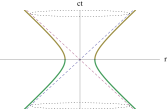
Figure 7: The classical and quantum corrected light cones of dynamical gravitons.

Curiously, the effect does not depend on $\xi$, i.e. it does not depend on whether the scalar is minimally or nonminimally coupled. This means that the effect (35) comes entirely from the kinetic term cubic vertex $-h^{\mu\nu}(\partial_{\mu}\varphi)(\partial_{\nu}\varphi)/2$. The classical light cones, as well as the quantum-shifted light cones, are shown in Fig. 7. Just as in the case of the photons, this graviton effect is very tiny (in fact, it is 40 times smaller than the effect found for the photons in Leonard:2012fs ), and thus it is uncertain whether it will ever be observed. From the structure of the light cone in Fig. 7, it is clear that the superluminality is not cumulative (it does not increase with distance). On the contrary, it becomes weaker as the distance increases. This can be understood as follows: the effect on larger scales is built primarily from quantum fluctuations on that scale, which have smaller amplitude than fluctuations on a smaller scale, and vice versa Yet, the effect is of some academic interest, as it is for the first time that a superluminal propagation of gravitons is inferred from quantum matter fluctuations. As a curiosity, we mention that a similar deformation of light cones has been observed in Hermitean Gravity of Ref. Mantz:2008hm , where a slight superluminal behavior was observed for particles with negative 4-momentum squared, $-p^{2}=[(E/c)^{2}-\vec{p}^{\,2}]>0$. Our effect is also different from the superluminal photon motion observed in curved geometries Drummond:1979pp ; Daniels:1995yw ; Daniels:1993yi , where the effects were calculated in a gradient expansion. No such approximation has been used here. Moreover, our results are manifestly gauge independent, and they are calculated within a gauge invariant formalism.

IV Summary and discussion

In this paper we perform one-particle irreducible (1PI) resummation of the one-loop vacuum fluctuations of nonminimally coupled, massless, scalar matter. Our main result (18) and (19) indicates that gravity gets strongly antiscreened on (super-)Planckian energies, supporting the hypothesis of asymptotic freedom, according to which gravity becomes weak on super-Planckian scales. Furthermore, we study how vacuum fluctuations affect graviton propagation. We find that gravitons moving in a sea of vacuum fluctuations are sped up, resulting in a slightly superluminal motion (see Fig. 7). However, the effect is too weak to be observable.

Antiscreening on short scales is such that the Bardeen gravitational potentials remain finite everywhere, also arbitrarily close to the origin. However, the Riemann curvature tensor still exhibits singularity at the origin, albeit this singularity is much milder ($R_{\mu\nu\rho\sigma}R^{\mu\nu\rho\sigma}\propto 1/r^{2}$) than the usual singularity of black hole space times (for which $R_{\mu\nu\rho\sigma}R^{\mu\nu\rho\sigma}\propto 1/r^{6}$). In addition, the Ricci scalar and Ricci tensor are also singular, which is not surprising since vacuum fluctuations act as matter. Since for (elementary) particles of sub-Planckian mass the Bardeen potentials remain small everywhere (see Figs. 5 and 6), our results may be trustable when applied to known elementary particles. For heavy particles (whose mass is comparable to or larger than the Planck mass), we also find qualitatively the same strong antiscreening. However, our results cannot be trusted here since, at short distances (closer to the would-be event horizon), the amplitude of the gravitational potentials becomes of the order 1 or larger (see Figs. 3 and 4), invalidating our linearized approach to gravitational perturbations. So, in order to obtain more reliable results also in this case, it is required to extend our methods beyond linear order in the gravitational fields, or work in coordinates in which perturbations remain small everywhere. But, this task is left for a future work.

A couple of remarks follow. It is believed that, just like quantum chromodynamics (QCD), quantum gravity is an asymptotically free theory, in the sense that in the far ultraviolet it decouples from matter fields and becomes weak. There is some evidence for the asymptotic safety program that in the UV quantum gravity develops correlations as if it were effectively a two-dimensional theory. This then implies that the corresponding spectrum is scale invariant, which may have relevance for generation of cosmological perturbations. Asymptotic freedom of QCD has led to the conjecture (which has in the meantime been confirmed by numerical simulations) that, at high temperatures, the QCD matter is in a state of a quark-gluon plasma, in which most of the quarks (those of a sufficiently high energy) move essentially free. A quite exciting possibility is that a similar scenario may be realized within gravity. One can then imagine a collection of gravitationally weakly interacting very closely packed particles which would make dense objects which – due to the gravitational asymptotic freedom – would not collapse into black holes, or at least would screen curvature singularities at the origin of black holes. Whether this picture is consistent with our understanding of quantum gravity remains to be seen and requires further investigation.

Our analysis in the Appendix contains results that are worth commenting on. The graviton vacuum polarization tensor of a massless nonminimally coupled scalar field has such a tensor structure that, when it acts on a graviton field, it yields gauge invariant field components. This result motivates the following conjecture:

1. Gauge invariance dictates the structure of the graviton vacuum polarization tensor induced by any massless matter or gravitational field at the one-loop order. The structure is a slight generalization of (2),

   $$\left[{}_{\mu\nu}\Pi_{\rho\sigma}^{\rm ret}\right](x;x^{\prime})=L_{\mu\nu\alpha\beta}\bigg{\{}\alpha D^{\alpha\beta}{}_{\rho\sigma}+\beta\eta^{\alpha\beta}D_{\rho\sigma}\bigg{\}}\partial^{4}\,\Big{\{}\Theta(\Delta t^{2}-\Delta r^{2})\Theta(\Delta t)\left[\ln|\mu^{2}(\Delta r^{2}-\Delta t^{2})|-1\right]\Big{\}}\,,\,$$

   where $\alpha$ and $\beta$ are field dependent constants and $D^{\rho\sigma}$ and $D_{\alpha\beta}^{\;\;\;\;\rho\sigma}$ are the derivative operators defined in (4) [if a field is massive, then the scalar function on the second line of (2) will be different, but on the light cone it will reduce to the one given in (2) and in the equation above]. The vacuum polarization tensor at higher loops will still have the same tensor structure, but scalar functions will generally be different.

Conversely, the structure of Eq. (1) is such that it is gauge invariant. Since this equation is linear in metric perturbations, it also means that it is gauge independent to the (linear) order considered. This can be shown as follows. Firstly, note that both the graviton vacuum polarization (2) and the Lichnerowicz operator (3) consist of operators $D_{\mu\nu}$ and $D_{\mu\nu\rho\sigma}$ defined in Eqs. (4). Now, since under an infinitesimal coordinate shift, $x^{\mu}\rightarrow x^{\mu}+\xi^{\mu}(x)$, where $\xi^{\mu}(x)$ is an infinitesimal function, to linear order the metric perturbation $h_{\mu\nu}$ transforms as $h_{\mu\nu}\rightarrow h_{\mu\nu}-2\partial_{(\mu}\xi_{\nu)}$. This then implies that, to linear order in $\xi^{\mu}$ we have

$$D^{\mu\nu}h_{\mu\nu}\rightarrow D^{\mu\nu}h_{\mu\nu}-2D^{\mu\nu}\partial_{\mu}\xi_{\nu}=D^{\mu\nu}h_{\mu\nu}\,,$$

and

$$D^{\mu\nu\rho\sigma}h_{\rho\sigma}\rightarrow D^{\mu\nu\rho\sigma}h_{\rho\sigma}-2D^{\mu\nu\rho\sigma}\partial_{\rho}\xi_{\sigma}=D^{\mu\nu\rho\sigma}h_{\rho\sigma}\,.$$

This immediately implies that the classical part of Eq. (1) is both gauge independent and gauge invariant. In the quantum part of (1) one can perform two partial integrations to move $D^{\mu\nu}$ and $D^{\mu\nu\rho\sigma}$ to act on $h_{\rho\sigma}$ under the $x^{\prime}$ integral, implying that – up to boundary terms – the whole equation can be written in a gauge invariant form. The invariance under some symmetry transformation of the vacuum polarization tensor can be checked by considering, for example, the vacuum polarization induced by the one-loop (Abelian or non-Abelian) gauge fields Capper:1979ej ; Capper:1978yf ; Capper:1974vb . An intricate gauge dependence in the one-loop gravitational potentials seen by a point particle was discussed in Refs. Dalvit:1997yc ; Gribouk:2003ks . It would be of interest to relate these results and to the ones presented in this work.

A fully covariant form for the vacuum polarization was presented in Jordan:1987wd and in Barvinsky:1987uw ; Barvinsky:1990up . Next we discuss how to connect our work to the covariant perturbation theory of Barvinsky and Vilkovisky Barvinsky:1987uw ; Barvinsky:1990up . Adapting Eq. (3.4) from Barvinsky:1990up to a nonminimally coupled scalar field in a Lorentzian space yields for the one-loop effective action

$$\Gamma_{\rm eff} = -\frac{1}{\kappa^{2}}\int d^{D}x\sqrt{-g}R$$

$$\hskip 0.0pt-\,\frac{1}{1920\pi^{2}}\int d^{D}x\sqrt{-g}\bigg{\{}R_{\alpha\beta}\Big{[}\Gamma(-\Box)\!+\!\frac{16}{15}\,\Big{]}R^{\alpha\beta}\!+30\Big{(}\xi\!-\!\frac{1}{6}\Big{)}^{2}R\Gamma(-\Box)R-\frac{1}{3}R\Gamma(-\Box)R-\frac{10}{3}\Big{(}\xi\!-\!\frac{29}{100}\Big{)}R^{2}\bigg{\}}\,,\quad$$

where we included the Einstein-Hilbert classical action and the finite part of the operator $\Gamma(-\Box)$ is

$$\Gamma(-\Box)=\!-\!\ln\Big{(}\frac{-\Box}{4\pi\mu^{2}}\Big{)}+2-\gamma_{E}\,.$$ (37)

In Eq. (IV) we took the values for the tensors from Eq. (3.4) that correspond to a nonminimally coupled scalar field, that is $\hat{P}=[(1/6)-\xi]R\hat{1}$ and ${\cal R}_{\mu\nu}=0$, and we evaluated the trace (${\rm tr}[\hat{1}]=1$). Note that in an Euclidean space the operator $\ln(-\Box/\mu^{2})$ in Eq. (3.4) of Ref. Barvinsky:1990up is well defined because the norm of the operator $-\Box$ is positive. This is however not the case in a Lorentzian space and hence extra care is needed to properly (uniquely) define the meaning of the nonlocal operator $\ln(-\Box/\mu^{2})$. The correspondence between the Euclidean result (37) and the Lorentzian in-in formulation (and in particular the representation of the nonlocal operator $\ln(-\Box/\mu^{2})$ in the in-in formalism) can be found, for example, in Ref. Lombardo:1996gp .

Next we observe that, to quadratic order in metric perturbation $h_{\mu\nu}$ around flat Minkowski space, the action (IV) becomes,

$$\Gamma_{\rm eff} = \frac{1}{2\kappa^{2}}\int d^{D}xh^{\mu\nu}L_{\mu\nu\rho\sigma}h^{\rho\sigma}$$

$$\hskip 0.0pt-\,\frac{1}{1920\pi^{2}}\int d^{D}xh^{\mu\nu}\bigg{\{}\Big{[}\Gamma(-\Box)\!+\!\frac{16}{15}\,\Big{]}L_{\mu\nu\alpha\beta}\Big{(}D^{\alpha\beta}_{\;\;\rho\sigma}-\frac{1}{2}\eta^{\alpha\beta}D_{\rho\sigma}\Big{)}$$

$$\hskip 0.0pt+\,\bigg{[}30\Big{(}\xi\!-\!\frac{1}{6}\Big{)}^{2}-\frac{1}{3}\bigg{]}\Gamma(-\Box)L_{\mu\nu\alpha\beta}\Big{(}-\eta^{\alpha\beta}D_{\rho\sigma}\Big{)}-\frac{10}{3}\Big{(}\xi\!-\!\frac{29}{100}\Big{)}L_{\mu\nu\alpha\beta}\Big{(}-\eta^{\alpha\beta}D_{\rho\sigma}\Big{)}\bigg{\}}h^{\rho\sigma}\,,\quad$$

where we made use of $R=D_{\mu\nu}h^{\mu\nu}+{\cal O}(h_{\alpha\beta}^{2})$, $R_{\alpha\beta}=D_{\alpha\beta\mu\nu}h^{\mu\nu}+{\cal O}(h_{\alpha\beta}^{2})$ and $D_{\mu\nu}$ and $D_{\alpha\beta\mu\nu}$ are defined in Eq. (4) and, in addition, we partially integrated twice and made use of Eqs. (25) and (26) from Ref. Marunovic:2011zw . Now, upon varying the action (IV) and setting it equal to the stress energy tensor of a point mass source $(1/2)\delta_{\mu}^{\;0}\delta_{\nu}^{\;0}M\delta^{3}(\vec{x}\,)$ we get,

$$h^{\alpha\beta\,(c)}=h^{\alpha\beta}\!+\frac{\kappa^{2}}{960\pi^{2}}\bigg{\{}\bigg{[}\!-\!\Gamma(-\Box)\!-\!\frac{16}{15}\,\bigg{]}D^{\alpha\beta}_{\;\;\rho\sigma}-\bigg{[}\frac{1}{6}\!+\!30\Big{(}\xi\!-\!\frac{1}{6}\Big{)}^{2}\bigg{]}\big{[}\!-\!\Gamma(-\Box)\big{]}\eta^{\alpha\beta}D_{\rho\sigma}\!-\!\frac{10}{3}\Big{(}\xi\!-\!\frac{9}{20}\Big{)}\eta^{\alpha\beta}D_{\rho\sigma}\bigg{\}}h^{\rho\sigma},\quad$$ (39)

where we made use of the fact that $h^{\rho\sigma\,(c)}$ is the classical metric that corresponds to the pointlike source [see Eq. (5)], which allowed us to remove the Lichnerowicz operator from Eq. (39). When the (real space) expression (39) is compared with the momentum space expression (50) we see that there is perfect agreement of the coefficients multiplying the logarithm $\ln(-\partial^{2}/\mu^{2})\rightarrow\ln(|(k^{0})^{2}-k^{2}|/\mu^{2})+$ (an imaginary part), while the coefficients of the local terms do not agree. These coefficients are not universal and can be adjusted by a suitable choice of local counterterms. A generalization of the Barvinsky-Vilkovisky results to massive field theories has been exacted in Refs. Avramidi:1989er ; Dalvit:1994gf which, of course, in the massless limit reproduce Eq. (39). In conclusion, we have shown that our one-loop expression for the metric perturbations around Minkowski background can be obtained from the more general expression derived in Refs. Barvinsky:1987uw ; Barvinsky:1990up . As regards the imaginary part of the operator (37), we note that the prescription used in the Appendix corresponds to the retarded boundary prescription, which is the appropriate (causal) prescription that automatically follows from the Schwinger-Keldysh formalism. An alternative prescription for the imaginary part corresponding to the retarded self-energy was given in Ref. Jordan:1987wd , where the author argued that the graviton self-energy can be represented in terms of the Feynman propagators.

Finally, it would be of interest to clarify what is the connection (if any) between the results of the asymptotic safety program (according to which quantum gravity in the ultraviolet becomes weak, and hence antiscreened) and the results presented in this work.

Appendix: Solving the integral equation for the gravitational field

Here we show how to solve the integral equation (6) for the (quantum) gravitational field $h^{\alpha\beta}(x)$,

$$h_{\alpha\beta}^{(c)}(x) = h_{\alpha\beta}(x)-\frac{\kappa^{2}}{7680\pi^{3}}\bigg{\{}D_{\alpha\beta}{}^{\rho\sigma}-\eta_{\alpha\beta}D^{\rho\sigma}\bigg{[}\frac{1}{6}+30\Big{(}\xi-\frac{1}{6}\Big{)}^{2}\bigg{]}\bigg{\}}F_{\rho\sigma}(x)\,,$$ (40)

where

$$F_{\rho\sigma}(x)=\partial^{4}\int d^{4}x^{\prime}\Theta(\Delta t^{2}-\Delta r^{2})\Theta(\Delta t)\left[\ln(\mu^{2}(\Delta t^{2}-\Delta r^{2}))-1\right]h_{\rho\sigma}(x^{\prime}).$$ (41)

Upon performing a spatial Fourier transform, Eq. (41) can be reduced to

$$F_{\rho\sigma}(\vec{k},t)=\frac{4\pi}{k}(\partial_{t}^{2}+k^{2})^{2}\int_{-\infty}^{t}dt^{\prime}\int_{0}^{\Delta t}d(\Delta r)\Delta r\sin(k\Delta r)\Big{[}\ln\Big{(}\mu^{2}(\Delta t^{2}-\Delta r^{2})\Big{)}-1\Big{]}h_{\rho\sigma}(\vec{k},t^{\prime})\,,$$ (42)

where $k=\|\vec{k}\|$ and

$$F_{\rho\sigma}(\vec{k},t)=\int d^{3}x{\rm e}^{-\imath\vec{k}\cdot\vec{x}}F^{\rho\sigma}(\vec{x},t)\,,\qquad h_{\rho\sigma}(\vec{k},t^{\prime})=\int d^{3}x{\rm e}^{-\imath\vec{k}\cdot\vec{x}}h_{\rho\sigma}(\vec{x},t^{\prime})\,.$$

The spatial integral can be reduced to $\Xi_{-1}(z,\zeta)$ defined in Ref. Prokopec:2003iu , Eqs. (45)-(50),

$$F_{\rho\sigma}(\vec{k},t)=\frac{4\pi}{k^{3}}(\partial_{t}^{2}+k^{2})^{2}\int_{-\infty}^{t}dt^{\prime}\Xi_{-1}(z,\zeta)h_{\rho\sigma}(\vec{k},t^{\prime})\,,$$ (43)

where $z=k\Delta t$, $\zeta=k/\mu$, $x=\Delta r/\Delta t$,

$$\Xi_{n}(z,\zeta)=z^{2}\int_{0}^{1}dxx\sin(zx)[2\ln(z/\zeta)+\ln(1-x^{2})+n]=[\sin(z)-z\cos(z)][2\ln(z/\zeta)+n]+z^{2}\xi(z)\,$$ (44)

and

$$\xi(z) = z^{2}\int_{0}^{1}dxx\sin(zx)\ln(1-x^{2})$$ (45)

$$= 2\sin(z)-[\cos(z)+z\sin(z)][{\rm si}(2z)+\pi/2]+[\sin(z)-z\cos(z)][{\rm ci}(2z)-\gamma_{E}-\ln(z/2)]\,,$$

with

$${\rm si}(z)=-\int_{z}^{\infty}\frac{\sin(t)dt}{t}=\int_{0}^{z}\frac{\sin(t)dt}{t}-\frac{\pi}{2}\,,\qquad{\rm ci}(z)=-\int_{z}^{\infty}\frac{\cos(t)dt}{t}=\int_{0}^{z}\frac{[\cos(t)-1]dt}{t}+\gamma_{E}+\ln(z)\,.$$

Now, since for small $z=k\Delta t$, $\Xi_{n}\propto z^{3}\ln(z)$, one can act with $\partial_{t}^{2}+k^{2}$ once without touching the upper limit of the time integral in (43) to obtain

$$F_{\rho\sigma}(\vec{k},t)=\frac{4\pi}{k}(\partial_{t}^{2}+k^{2})\int_{-\infty}^{t}dt^{\prime}(\partial_{z}^{2}+1)\Xi_{-1}(z,\zeta)h_{\rho\sigma}(\vec{k},t^{\prime})\,,$$ (46)

where

$$(\partial_{z}^{2}+1)\Xi_{n}(z,\zeta)=\sin(z)[2\ln(z/\zeta)+(n+1)+{\rm ci}(2z)-\gamma_{E}-\ln(2z)]-\cos(z)[{\rm si}(2z)+\pi/2]$$

Next, upon observing that,

$$(\partial_{z}^{2}+1)^{2}\Xi_{n}(z,\zeta)=4\frac{\cos(z)-1}{z}+4\partial_{z}[\ln(2z/\zeta)+(n+1)/2]\,,$$

one concludes that (46) can be recast as

$$F_{\rho\sigma}(\vec{k},t)=16\pi\Bigg{[}\int_{-\infty}^{t}dt^{\prime}\frac{\cos(k\Delta t)-1}{\Delta t}+\partial_{t}\int_{-\infty}^{t}dt^{\prime}\ln(2\mu\Delta t)\Bigg{]}h_{\rho\sigma}(\vec{k},t^{\prime})\,.$$ (47)

We shall now argue that in the second integral, one can move the derivative $\partial_{t}$ to act as $\partial_{t^{\prime}}$ on $h_{\rho\sigma}(\vec{k},t^{\prime})$. Notice firstly that one can write $\ln(2\mu\Delta t)=-\partial_{t^{\prime}}\{\Delta t[\ln(2\mu\Delta t)-1]\}$, and then one can partially integrate $\partial_{t^{\prime}}$ to act on $h_{\rho\sigma}(\vec{k},t^{\prime})$. Formally, this will generate an infinite contribution from the initial state at $t^{\prime}\rightarrow-\infty$. This infinite contribution can be regulated away, if one assumes that $h_{\rho\sigma}(\vec{k},t^{\prime})$ gets adiabatically switched on as $h_{\rho\sigma}(\vec{k},t^{\prime})\propto{\rm e}^{\epsilon t^{\prime}}$ as $t^{\prime}\rightarrow-\infty$. After this, one can act with $\partial_{t}$, and the second integral becomes $\int_{-\infty}^{t}dt^{\prime}\ln(2\mu\Delta t)\partial_{t^{\prime}}h_{\rho\sigma}(\vec{k},t^{\prime})$. This expression is now prepared for a Fourier transform over time. By noting that

$$h_{\rho\sigma}(\vec{k},t^{\prime})=\int\frac{dk^{0}}{2\pi}{\rm e}^{-\imath k^{0}t^{\prime}}h_{\rho\sigma}(k^{\mu})={\rm e}^{-\imath k^{0}t}\int\frac{dk^{0}}{2\pi}{\rm e}^{\imath k^{0}\Delta t}h_{\rho\sigma}(k^{\mu})\,,$$

$F_{\rho\sigma}(k^{\mu})$ can be written in momentum space as,

$$F_{\rho\sigma}(k^{\mu})=-8\pi\bigg{[}\ln\bigg{(}\frac{|(k^{0})^{2}-k^{2}|}{4\mu^{2}}\bigg{)}+2\gamma_{E}-\frac{\imath\pi}{2}\Big{(}{\rm sign}(k^{0}+k)+{\rm sign}(k^{0}-k)\Big{)}\bigg{]}h_{\rho\sigma}(k^{\mu})\,,$$ (48)

where we made use of the following integrals,

$$\int_{0}^{\infty}d\Delta t{\rm e}^{\imath k^{0}\Delta t}\frac{\cos(k\Delta t)-1}{\Delta t} = \frac{1}{2}\ln\bigg{(}\frac{|k^{0}|^{2}}{|(k^{0})^{2}-k^{2}|}\bigg{)}+\frac{\imath\pi}{4}\Big{[}{\rm sign}(k^{0}+k)+{\rm sign}(k^{0}-k)-2{\rm sign}(k^{0})\Big{]}\,,$$

$$\int_{0}^{\infty}d\Delta t{\rm e}^{\imath k^{0}\Delta t}\ln(2\mu\Delta t) = -\frac{\imath}{k^{0}}\bigg{[}\ln\bigg{(}\frac{|k^{0}|}{2\mu}\bigg{)}-\frac{\imath\pi}{2}{\rm sign}(k^{0})+\gamma_{E}\bigg{]}\,.$$

Now making use of $(1/2)[{\rm sign}(k^{0}+k)+{\rm sign}(k^{0}-k)]={\rm sign}(k^{0})\theta((k^{0})^{2}-k^{2})$ we see that (48) can be also written as

$$F_{\rho\sigma}(k^{\mu})=-8\pi\bigg{[}\ln\bigg{(}\frac{-(k^{0}+\imath\epsilon)^{2}+k^{2}}{4\mu^{2}}\bigg{)}+2\gamma_{E}\bigg{]}h_{\rho\sigma}(k^{\mu})\,.$$ (49)

This structure of the retarded one-loop self-energy agrees with e.g. Eq. (E9) in Appendix E of Ref. Koksma:2009wa , where various components of the one-loop self-energy within the Schwinger-Keldysh in-in formalism are constructed for an interacting scalar field theory. It is not clear to us how to relate (49) to the prescription used in Jordan:1987wd , where it was argued that the retarded self-energy is obtained by taking the real part of the contribution $\propto\ln[(-(k^{0})^{2}+k^{2}-\imath\epsilon)/\mu^{2}]=\ln\big{[}|(k^{0})^{2}-k^{2}|/\mu^{2}\big{]}-\imath\pi\theta\big{(}(k^{0})^{2}-k^{2}\big{)}$, whereby the real, causal part should be taken after the momentum integration. The result (48) or (49) for the retarded self-energy is simpler and more transparent, and we shall therefore use it in the rest of this work. Inserting (48) into Eq. (40) and transforming into momentum space one gets,

$$h_{\alpha\beta}^{(c)}(k^{\mu}) = h_{\alpha\beta}(k^{\mu})+\frac{\kappa^{2}}{960\pi^{2}}\bigg{\{}\tilde{D}_{\alpha\beta}{}^{\rho\sigma}-\eta_{\alpha\beta}\tilde{D}^{\rho\sigma}\bigg{[}\frac{1}{6}+30\Big{(}\xi-\frac{1}{6}\Big{)}^{2}\bigg{]}\bigg{\}}$$ (50)

$$\times\,\bigg{[}\ln\bigg{(}\frac{|(k^{0})^{2}-k^{2}|}{4\mu^{2}}\bigg{)}+2\gamma_{E}-\frac{\imath\pi}{2}\Big{(}{\rm sign}(k^{0}+k)+{\rm sign}(k^{0}-k)\Big{)}\bigg{]}h_{\rho\sigma}(k^{\mu})\,,$$

where [cf. Eq. (4)]

$$\tilde{D}^{\rho\sigma}=-k^{\rho}k^{\sigma}+\eta^{\rho\sigma}(k^{\mu}k_{\mu})\;,\qquad\tilde{D}_{\alpha\beta}^{\;\;\;\;\rho\sigma}=-k_{(\alpha}\delta_{\beta)}^{\;\;(\rho}k^{\sigma)}+\frac{1}{2}\delta_{\alpha}^{\;\;(\rho}\delta^{\sigma)}_{\;\;\beta}(k^{\mu}k_{\mu})+\frac{1}{2}\eta^{\rho\sigma}k_{\alpha}k_{\beta}\,.$$ (51)

Next it is useful to act with the two operators (51) on $h_{\rho\sigma}$. It is interesting to note that these generate only gauge invariant combinations of components of $h_{\rho\sigma}$. For example,

$$\tilde{D}^{\rho\sigma}h_{\rho\sigma}(k^{\mu})=2k^{2}\Phi(k^{\mu})+2\big{[}3(k^{0})^{2}-2k^{2}\big{]}\Psi(k^{\mu})\,,$$ (52)

where

$$\Psi=-\frac{1}{6}(h+k^{2}\tilde{h})\,,\qquad\Phi=-\frac{1}{2}(h_{00}+2\imath k^{0}\sigma-(k^{0})^{2}\tilde{h})\,,$$ (53)

and we have made use of a Helmholtz decomposition of $h_{\mu\nu}$,

$$h_{0i}=n_{i}^{T}+\imath k_{i}\sigma\,,\qquad\ h_{ij}=\frac{\delta_{ij}}{3}h-\Big{(}k_{i}k_{j}-\frac{\delta_{ij}}{3}k^{2}\Big{)}\tilde{h}+\imath(k_{i}h_{j}^{T}+k_{j}h_{i}^{T})+h_{ij}^{TT}$$ (54)

where $n_{i}^{T},h_{i}^{T}$ and $h_{ij}^{TT}$ are transverse, $k^{i}n_{i}^{T}=0=k^{i}h_{i}^{T}$, $k^{i}h_{ij}^{TT}=0=h_{ij}^{TT}k^{j}$, and $h_{ij}^{TT}$ is in addition traceless, $h_{ii}^{TT}=0$ and $k\equiv\|\vec{k}\|$. Apart from the Bardeen potentials, there is one gauge invariant vector and one gauge invariant tensor,

$$\tilde{n}_{i}^{T}=n_{i}^{T}+\imath k^{0}h_{i}^{T}\,,\qquad h_{ij}^{TT}\,,$$ (55)

such that there are in total six gauge invariant fields, which means that four out of the ten components of $h_{\mu\nu}$ are gauge dependent, i.e. they change if one performs a coordinate shift $x^{\mu}\rightarrow x^{\mu}+\xi^{\mu}(x)$, where $\xi^{\mu}(x)$ is a small coordinate shift, of the order of metric components $h_{\mu\nu}$. Note that $h_{ij}^{TT}$ is on its own gauge invariant, and represents the two dynamical, tensorial degrees of freedom of gravity (gravitational waves).

Similarly, the action of the second operator in (51) yields gauge invariant quantities only,

$$\tilde{D}_{00}^{\;\;\;\;\rho\sigma}h_{\rho\sigma} = -k^{2}\Phi-3(k^{0})^{2}\Phi\,,$$

$$\tilde{D}_{0i}^{\;\;\;\;\rho\sigma}h_{\rho\sigma} = \frac{1}{2}k^{2}\tilde{n}_{i}^{T}+2k^{0}k_{i}\Psi=\tilde{D}_{i0}^{\;\;\;\;\rho\sigma}h_{\rho\sigma}\,,$$

$$\tilde{D}_{ij}^{\;\;\;\;\rho\sigma}h_{\rho\sigma} = k_{i}k_{j}\Phi+\big{[}-k_{i}k_{j}-\delta_{ij}\big{(}-(k^{0})^{2}+k^{2}\big{)}\big{]}\Psi-k^{0}k_{(i}\tilde{n}_{j)}^{T}+\frac{1}{2}\big{[}-(k^{0})^{2}+k^{2}\big{]}h_{ij}^{TT}\,.$$ (56)

Since the Lichnerowicz operator (3) of the classical equation of motion for $h_{\rho\sigma}^{(c)}$ is a linear combination of $D^{\rho\sigma}$ and $D_{\alpha\beta}^{\;\;\;\;\rho\sigma}$, it also yields gauge invariant quantities in the equation of motion. This observation was already made in our earlier work Marunovic:2011zw . There is however a much stronger statement one can make: the structure of the equation that includes the graviton vacuum polarization (1) and (2) is also gauge invariant (at least to the order the equation is written). This property can be used to our advantage and study quantum effects in a fully gauge invariant fashion.

Since all components of the vacuum polarization are gauge invariant, one can use the Helmholtz decomposition (54) and simply combine the component equations (50) into gauge invariant combinations according to (53) and (55), resulting in the following gauge invariant equations:

$$\Phi^{(c)} = \Phi+{\cal K}\Big{\{}\big{(}-(k^{0})^{2}+k^{2}\big{)}\Phi+\Big{[}\frac{1}{6}+30\Big{(}\xi-\frac{1}{6}\Big{)}^{2}\Big{]}\Big{[}-2k^{2}\Phi+2\big{(}-3(k^{0})^{2}+2k^{2}\big{)}\Psi\Big{]}\Big{\}}\,,$$ (57)

$$\Psi^{(c)} = \Psi+{\cal K}\Big{\{}\big{(}-(k^{0})^{2}+k^{2}\big{)}\Psi-\Big{[}\frac{1}{6}+30\Big{(}\xi-\frac{1}{6}\Big{)}^{2}\Big{]}\Big{[}-2k^{2}\Phi+2\big{(}-3(k^{0})^{2}+2k^{2}\big{)}\Psi\Big{]}\Big{\}}\,,$$ (58)

$${\tilde{n}}_{i}^{T(c)} = \tilde{n}_{i}^{T}+{\cal K}\big{(}-(k^{0})^{2}+k^{2}\big{)}\tilde{n}_{i}^{T}$$ (59)

$${h_{ij}^{TT}}^{(c)} = h_{ij}^{TT}+{\cal K}\big{(}-(k^{0})^{2}+k^{2}\big{)}h_{ij}^{TT}\,,$$ (60)

where we defined

$${\cal K}=\frac{\kappa^{2}}{1920\pi^{2}}\bigg{[}\ln\bigg{(}\frac{|(k^{0})^{2}-k^{2}|}{4\mu^{2}}\bigg{)}+2\gamma_{E}-\frac{\imath\pi}{2}\Big{(}{\rm sign}(k^{0}+k)+{\rm sign}(k^{0}-k)\Big{)}\bigg{]}\,.$$ (61)

The last two equations (59) and (60) are easily solved,

$${\tilde{n}}_{i}^{T}(k^{\mu}) = \frac{{\tilde{n}}_{i}^{T(c)}(k^{\mu})}{1+\big{(}-(k^{0})^{2}+k^{2}\big{)}{\cal K}(k^{\mu})}\,,$$ (62)

$${h_{ij}^{TT}}(k^{\mu}) = \frac{{h_{ij}^{TT}}^{(c)}(k^{\mu})}{1+{\cal K}(k^{\mu})\big{(}-(k^{0})^{2}+k^{2}\big{)}}\,,$$ (63)

and tell us that the effect of one-loop vacuum polarization for the vector and tensor perturbations can be absorbed into a finite wave function renormalization; i.e. vacuum polarization changes the amplitude of the gravitational wave. The effect is however tiny, since on shell, where $-(k^{0})^{2}+k^{2}=0$, the effect vanishes. That means that, when there are no classical gravitational waves, quantum effects of scalar vacuum fluctuations do not generate any. The same holds for vector perturbations: if they are zero classically, they will not be generated by fluctuating scalar fields. Because the structure of vacuum polarization is dictated by gauge invariant tensor structures, we expect the same conclusions concerning gauge invariant vector and tensor perturbations to hold for arbitrary fields: the quantum effects of the fluctuations will just renormalize the wave function.

The structure of the scalar equations (57) and (58) is more complex, because they in general couple. Note that the equation for the sum of the Bardeen potentials is particularly simple,

$$\Phi^{(c)}+\Psi^{(c)}=\Phi+\Psi+{\cal K}\big{(}-(k^{0})^{2}+k^{2}\big{)}(\Phi+\Psi)\,,$$ (64)

whose solution is of the same form as that of the vector (62) and tensor perturbations (63),

$$\Phi+\Psi=\frac{\Phi^{(c)}+\Psi^{(c)}}{1+{\cal K}\big{(}-(k^{0})^{2}+k^{2}\big{)}}\,;$$ (65)

i.e. the effect of loop fluctuations of quantum fields on the sum $\Phi+\Psi$ is just a finite renormalization of its amplitude, which vanishes on shell.

It is, of course, possible to decouple the two Bardeen potentials (57) and (58). A convenient way of writing the decoupled equations is

$$\Phi = \frac{\Phi^{(c)}}{1-5(1-6\xi)^{2}(k^{\mu}k_{\mu}){\cal K}}-\Big{(}\frac{2}{3}k^{2}-(k^{0})^{2}\Big{)}{\cal K}\Bigg{[}\frac{5(1-6\xi)^{2}}{1-5(1-6\xi)^{2}(k^{\mu}k_{\mu}){\cal K}}+\frac{1}{1+(k^{\mu}k_{\mu}){\cal K}}\Bigg{]}(\Phi^{(c)}+\Psi^{(c)})\,,\qquad$$ (66)

$$\Psi = \frac{\Psi^{(c)}}{1-5(1-6\xi)^{2}(k^{\mu}k_{\mu}){\cal K}}-\frac{1}{3}k^{2}{\cal K}\Bigg{[}\frac{5(1-6\xi)^{2}}{1-5(1-6\xi)^{2}(k^{\mu}k_{\mu}){\cal K}}+\frac{1}{1+(k^{\mu}k_{\mu}){\cal K}}\Bigg{]}(\Phi^{(c)}+\Psi^{(c)})\,.$$ (67)

This means that each of the two quantum-corrected Bardeen potentials depend on both classical Bardeen potentials. Since in general relativity, the classical potentials sourced by a point mass (or a scalar field) are equal $\Phi^{(c)}=\Psi^{(c)}$, Eqs. (66) and (67) further simplify to

$$\Phi = \Phi^{(c)}\Bigg{[}-\frac{1}{3}\frac{1-10(1-6\xi)^{2}(k^{0})^{2}{\cal K}}{1-5(1-6\xi)^{2}(k^{\mu}k_{\mu}){\cal K}}+\frac{2}{3}\frac{2+(k^{0})^{2}{\cal K}}{1+(k^{\mu}k_{\mu}){\cal K}}\Bigg{]}\,,\qquad$$ (68)

$$\Psi = \Phi^{(c)}\Bigg{[}\frac{1}{3}\frac{2-5(1-6\xi)^{2}(k^{0})^{2}{\cal K}}{1-5(1-6\xi)^{2}(k^{\mu}k_{\mu}){\cal K}}+\frac{1}{3}\frac{1-(k^{0})^{2}{\cal K}}{1+(k^{\mu}k_{\mu}){\cal K}}\Bigg{]}\,.$$ (69)

For a point stationary mass we have $\Phi^{(c)}=\Psi^{(c)}=4\pi G_{N}M/k^{2}$. These equations are now used to obtain the static limit of a (one-loop) quantum corrected gravitational response to a point mass in the main text.

References

- (1) A. Marunović and T. Prokopec, “Time transients in the quantum corrected Newtonian potential induced by a massless nonminimally coupled scalar field,” Phys. Rev. D 83 (2011) 104039 [arXiv:gr-qc/1101.5059].
- (2) J. F. Donoghue, “General Relativity As An Effective Field Theory: The Leading Quantum Corrections,” Phys. Rev. D 50 (1994) 3874 [arXiv:gr-qc/9405057].
- (3) J. F. Donoghue, “Leading quantum correction to the Newtonian potential,” Phys. Rev. Lett. 72 (1994) 2996 [arXiv:gr-qc/9310024].
- (4) H. W. Hamber and S. Liu, “On the quantum corrections to the Newtonian potential,” Phys. Lett. B 357, 51 (1995) [arXiv:hep-th/9505182].
- (5) A. Akhundov, S. Bellucci, A. Skiekh, ”Gravitational interaction to one loop in effective quantum gravity,” Phys. Lett. B 395, 16-23 (1997) [arXiv:gr-qc/9611018].
- (6) N. E. J. Bjerrum-Bohr, “Leading quantum gravitational corrections to scalar QED,” Phys. Rev. D 66 (2002) 084023 [arXiv:hep-th/0206236].
- (7) N. E. J. Bjerrum-Bohr, J. F. Donoghue and B. R. Holstein, “Quantum gravitational corrections to the nonrelativistic scattering potential of two masses,” Phys. Rev. D 67 (2003) 084033 [Erratum-ibid. D 71 (2005) 069903] [arXiv:hep-th/0211072].
- (8) N. E. J. Bjerrum-Bohr, J. F. Donoghue and B. R. Holstein, “Quantum corrections to the Schwarzschild and Kerr metrics,” Phys. Rev. D 68 (2003) 084005 [Erratum-ibid. D 71 (2005) 069904] [arXiv:hep-th/0211071].
- (9) M. S. Butt, ”Leading quantum gravitational corrections to QED”, Phys. Rev. D 74 (2006) 125007 [arXiv:gr-qc:/0605137].
- (10) Sven Faller, ”Effective field theory of gravity: Leading quantum gravitational corrections to Newton’s and Coulomb’s laws”, Phys. Rev. D 77 (2008) 124039 [arXiv:hep-th/0708.1701].
- (11) D. A. R. Dalvit, F. D. Mazzitelli, “Running coupling constants, Newtonian potential and nonlocalities in the effective action,” Phys. Rev. D50 (1994) 1001-1009. [arXiv:gr-qc/9402003].
- (12) A. Satz, F. D. Mazzitelli, E. Alvarez, “Vacuum polarization around stars: Nonlocal approximation,” Phys. Rev. D71 (2005) 064001. [arXiv:gr-qc/0411046].
- (13) S. Park, R. P. Woodard, “Scalar Contribution to the Graviton Self-Energy during Inflation” [arXiv:gr-qc/1101.5804].
- (14) D. M. Capper, “A General Gauge Graviton Loop Calculation,” J. Phys. A A 13 (1980) 199.
- (15) D. M. Capper and M. A. Namazie, “A General Gauge Calculation Of The Graviton Selfenergy,” Nucl. Phys. B 142 (1978) 535.
- (16) M. Reuter, “Nonperturbative evolution equation for quantum gravity,” Phys. Rev. D 57 (1998) 971 [arXiv:hep-th/9605030].
- (17) S. Weinberg, Ultraviolet Divergences In Quantum Theories Of Gravitation. In General Relativity: An Einstein centenary survey. Eds. S. W. Hawking and W. Israel, Cambridge University Press (1979), p.790
- (18) M. Reuter and F. Saueressig, “Quantum Einstein Gravity,” [arXiv:hep-th/1202.2274].
- (19) M. Niedermaier, “The Asymptotic safety scenario in quantum gravity: An Introduction,” Class. Quant. Grav. 24 (2007) R171 [arXiv:gr-qc/0610018].
- (20) A. O. Barvinsky and G. A. Vilkovisky, “Beyond the Schwinger-Dewitt Technique: Converting Loops Into Trees and In-In Currents,” Nucl. Phys. B 282 (1987) 163.
- (21) A. O. Barvinsky and G. A. Vilkovisky, “Covariant perturbation theory. 2: Second order in the curvature. General algorithms,” Nucl. Phys. B 333 (1990) 471.
- (22) A. Satz, A. Codello and F. D. Mazzitelli, “Low energy Quantum Gravity from the Effective Average Action,” Phys. Rev. D 82 (2010) 084011 [arXiv:1006.3808 [hep-th]].
- (23) G. T. Horowitz, “Semiclassical Relativity: The Weak Field Limit,” Phys. Rev. D 21 (1980) 1445.
- (24) R. D. Jordan, “Stability Of Flat Space-time In Quantum Gravity,” Phys. Rev. D 36 (1987) 3593.
- (25) Sean M. Carroll, ”Spacetime and Geometry: An Introduction to General relativity,” Addison Wesley, 2004.
- (26) K. E. Leonard and R. P. Woodard, “Graviton Corrections to Maxwell’s Equations,” Phys. Rev. D 85 (2012) 104048 [arXiv:gr-qc/1202.5800].
- (27) C. Mantz and T. Prokopec, “Hermitian Gravity and Cosmology,” [arXiv:gr-qc/0804.0213].
- (28) I. T. Drummond and S. J. Hathrell, “QED Vacuum Polarization in a Background Gravitational Field and Its Effect on the Velocity of Photons,” Phys. Rev. D 22 (1980) 343.
- (29) R. D. Daniels and G. M. Shore, “’Faster than light’ photons and rotating black holes,” Phys. Lett. B 367 (1996) 75 [arXiv:gr-qc/9508048].
- (30) R. D. Daniels and G. M. Shore, “’Faster than light’ photons and charged black holes,” Nucl. Phys. B 425 (1994) 634 [arXiv:hep-th/9310114].
- (31) T. Prokopec and R. P. Woodard, “Dynamics of superhorizon photons during inflation with vacuum polarization,” Annals Phys. 312 (2004) 1 [arXiv:gr-qc/0310056].
- (32) D. M. Capper and M. R. Medrano, “Gravitational Slavnov-Ward identities,” Phys. Rev. D 9 (1974) 1641.
- (33) D. A. R. Dalvit and F. D. Mazzitelli, “Geodesics, gravitons and the gauge fixing problem,” Phys. Rev. D 56 (1997) 7779 [hep-th/9708102].
- (34) T. S. Gribouk, K. A. Kazakov and P. I. Pronin, “Gauge dependence of effective gravitational field. 2. Point - like measuring device,” Phys. Rev. D 69 (2004) 024005 [hep-th/0306233].
- (35) F. C. Lombardo and F. D. Mazzitelli, “Einstein-Langevin equations from running coupling constants,” Phys. Rev. D 55 (1997) 3889 [gr-qc/9609073].
- (36) J. F. Koksma, T. Prokopec and M. G. Schmidt, “Decoherence in an Interacting Quantum Field Theory: The Vacuum Case,” Phys. Rev. D 81 (2010) 065030 [arXiv:0910.5733 [hep-th]].
- (37) J. F. Koksma, T. Prokopec and M. G. Schmidt, “Decoherence in an Interacting Quantum Field Theory: Thermal Case,” Phys. Rev. D 83 (2011) 085011 [arXiv:1102.4713 [hep-th]].
- (38) I. G. Avramidi, “Covariant Studies Of Nonlocal Structure Of Effective Action. (in Russian),” Sov. J. Nucl. Phys. 49 (1989) 735 [Yad. Fiz. 49 (1989) 1185].