Spectral dimension flow on continuum random multigraph

Abstract

We review a recently introduced effective graph approximation of causal dynamical triangulations (CDT), the multigraph ensemble. We argue that it is well suited for analytical computations and that it captures the physical degrees of freedom which are important for the reduction of the spectral dimension as observed in numerical simulations of CDT. In addition multigraph models allow us to study the relationship between the spectral dimension and the Hausdorff dimension, thus establishing a link to other approaches to quantum gravity.

1 Introduction

The causal dynamical triangulation (CDT) approach to quantum gravity (see Ambjørn et al. (2005) and Ambjørn et al. (2012) for a recent review) is a non-perturbative approach which employs lattice methods; the path integral is approximated as a sum over discretised (triangulated) geometries (i.e. dynamical triangulations) with a time foliation structure (the causal assumption). Computer simulations carried out in four-dimensional CDT revealed an intriguing result Ambjørn et al. (2005): a reduction of the spectral dimension from 4 at large scales to 2 at small scales where quantum effects are important. Thereafter other approaches to quantum gravity also observed this phenomenon Lauscher and Reuter (2005); Hořava (2009); Modesto (2009); Modesto and Nicolini (2010). However studying higher-dimensional CDT and its continuum limit is a difficult task and little progress has been made to analytically explain the results of the numerical simulations from the graph point of view. Certain fractal properties of two-dimensional (C)DTs, e.g. dimensionality, were studied with random walks on random geometries Ambjørn et al. (1997) and graphs Durhuus et al. (2009). We pursue these ideas further by developing a formalism to study random walks on multigraphs and arguing why the latter serves as realistic model to describe dimensional reduction in CDT.

The main notion of dimensionality we use is the spectral dimension ${d_{s}}$. It is related to a diffusion process (or random walk) on a geometric object defined by $p(t)\sim t^{-{d_{s}}/2}$ as $t\to\infty$, where $p(t)$ is the probability that a simple random walker returns to its origin after time $t$. An equivalent and sometimes more efficient way to study the spectral dimension is through the generating function of return probabilities defined as $Q(x)=\sum_{t=0}^{\infty}p(t)(1-x)^{t/2}\sim x^{-1+{d_{s}}/2}$ as $x\to 0$ provided it diverges in this limit. Divergence of $Q(x)$ implies that ${d_{s}}\leq 2$ and the random walk is recurrent, i.e. the probability to return to the origin is one. For non-recurrent (transient) random walks there is a finite probability that the random walker escapes to infinity, in this case $Q(x)$ is finite and the spectral dimension is defined through the first diverging derivative of $Q(x)$, i.e. $Q^{(k)}(x)\sim x^{-(k+1)+{d_{s}}/2}$ as $x\to 0$ for $2k\leq{d_{s}}<2(k+1)$.

A second definition of dimensionality on fractal geometries is the Hausdorff dimension, ${d_{H}}$, defined by the volume growth of a ball of radius $N$ centred on a fixed vertex, i.e. $B_{N}\sim N^{{d_{H}}}$ as $N\to\infty.$ Both definitions are valid provided that the limits exist and results for both the ensemble average and almost all graphs can be found in principle.

It is known Coulhon (1999) that for fixed graphs the Hausdorff and spectral dimensions (under certain conditions) satisfy the inequalities

$${d_{H}}\geq{d_{s}}\geq\frac{2{d_{H}}}{1+{d_{H}}}$$ (1)

which are also true for some random graphs. We will present instructive examples of such random graphs and further comment on this relation in the next sections.

2 the multigraph approximation

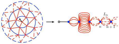
Figure 1: Illustration of how to obtain a multigraph from a causal triangulation.

The time foliation of $(d+1)$-dimensional causal triangulations implies a topology $I\times\Sigma^{d}$, where $d$ is the spatial dimension. The triangulation is made of triangles and their higher-dimensional analogues ($(d+1)$-simplices) which connect the $d$-dimensional spatial hyper-surfaces. A multigraph $M$ is defined by introducing a mapping which acts on a rooted infinite causal triangulation $C$ by collapsing all space-like edges at a fixed distance $k$, $k\geq 1$ from the root and identifying all vertices at this distance $k$. In the resulting multigraph a vertex $k$ has neighbours $k\pm 1$, except the vertex $0$ (the root $r$) which has $1$ as a neighbour, and there are $L_{k}(M)\geq 1$ (time-like) edges connecting $k$ and $k+1$ (see Figure 1). A random walker at vertex $k$ moves to $k+1$ with probability $p_{k}(M)=L_{k}/(L_{k-1}+L_{k})$ and to $k-1$ with probability $1-p_{k}(M)$. Note that the walker leaves the root to vertex 1 with probability one.

Denote $\eta_{M_{k}}\equiv Q_{M_{k}}/L_{k}$, where $M_{k}$ is the multigraph obtained from $M$ by removing the first $k$ vertices and the edges attached to them and relabelling the remaining graph. Then the generating function $Q_{M_{k}}$ follows the recursion relation Durhuus et al. (2009)

$$\eta_{M_{k}}(x)=\eta_{M_{k+1}}(x)+\frac{1}{L_{k}}-xL_{k}\eta_{M_{k}}(x)\eta_{M_{k+1}}(x).$$ (2)

3 The two-dimensional model

A two dimensional model of causal triangulations, the uniform infinite causal triangulation (UICT), was studied in Durhuus et al. (2009); Giasemidis et al. (2012a). Due to a bijection between causal triangulations and planar trees, the UICT - in essence a CDT at criticality - has the same measure as the generic random tree which can be viewed as a critical Galton-Watson process (with variance ${f^{U}}^{\prime\prime}(1)=2b/(1-b)$, where $b$ controls the variance of the offspring probabilities) conditioned on non-extinction. Furthermore, by construction the multigraph ensemble inherits its measure from the UICT. There is a number of analytical results which follow from UICT Durhuus et al. (2009). First, the ensemble average of the number of edges at distance $N$ from the root and the volume of a ball of radius $N$ is given by

$$\left\langle L_{N}\right\rangle_{\mu} = N{f^{U}}^{\prime\prime}(1)+1,\qquad n\geq 1,$$ (3)

$$\left\langle B_{N}\right\rangle_{\mu} \equiv \left\langle\sum_{k=0}^{N-1}L_{k}\right\rangle_{\mu}={\frac{1}{2}}N(N-1){f^{U}}^{\prime\prime}(1)+N,\qquad N\geq 1,$$ (4)

which implies ${d_{H}}=2$. Furthermore it is analytically proven in Durhuus et al. (2009) that $L_{N}$ is bounded above by logarithmic fluctuations around the average for almost all graphs in the ensemble, i.e. for almost all graphs

$$L_{N}\leq cN\log N$$ (5)

for large $N$, where $c>1$. In other words, the number of space-like edges at finite height $N$, $|S_{N}|$, remains finite since $L_{N}=|S_{N}|+|S_{N+1}|$. Thus omitting the space-like edges in the reduced model does not affect the random walk at large times and therefore the value of the spectral dimension of the causal triangulation. This turns to be a crucial point in our arguments in next section.

To understand further features of the multigraph approximation we introduce the notion of graph resistance $R_{G}$. It is defined by considering the graph as an electric network where each edge has resistance one Lyons and Peres (2011). One distinguishes two cases: The recurrent case (${d_{s}}\leq 2$) where a random walker “faces” infinite resistance to escape to infinity and returns to the root with probability 1; and the transient (or non-recurrent) case (${d_{s}}\geq 2$) where finite resistance to infinity implies return probability strictly less than one.

By Rayleigh’s monotonicity law the resistance from the root to infinity of the two-dimensional causal triangulation $R_{CT}$ is bounded by $R_{M}\leq R_{CT}\leq R_{{\emph{t}ree}}$, where $R_{M}$ and $R_{{\emph{t}ree}}$ are the resistance of the corresponding multigraph and tree respectively. Given that the resistance of recurrent multigraphs is infinite this inequality implies that the two-dimensional UICT is recurrent and ${d_{s}}\leq 2$ almost surely. Furthermore it implies that the recurrent multigraph ensemble and the generic tree ensemble are two extreme cases used to bound the spectral dimension of UICT and saturate the left and right hand side of (1) respectively (note that all the above graphs have ${d_{H}}=2$ and ${d_{s}}(GT)=4/3$ Durhuus et al. (2009, 2006)). It is believed that the spectral dimension of UICT is two and that thus multigraphs provide a tight bound.

In addition it was argued in Giasemidis et al. (2012a) the parameter $b$ introduced above is related to a CDT with an additional term in the action proportional to the absolute value of the scalar curvature $\sum_{\upsilon}|R_{\upsilon}|$ with a coupling constant $-\log b$. This term allows us to describe a scale dependent spectral dimension in the recurrent multigraph model. A scale dependent spectral dimension on graphs was studied before in Atkin et al. (2011) in the context of random combs. The measure of the multigraph ensemble depends on a characteristic distance $\Lambda=b^{-1}$ and the continuum limit is defined by taking the lattice spacing $a\to 0$

$$\tilde{Q}(\xi,\lambda)=\lim_{a\to 0}a^{1/2}\left\langle Q(x=a\xi;\Lambda=a^{-1/2}\lambda^{1/2})\right\rangle_{\mu}\sim\begin{cases}\xi^{-1/2},&\xi>>\lambda^{-1},\\ \lambda^{1/2}|\log\lambda\xi|,&\xi<<\lambda^{-1},\end{cases}$$ (6)

which implies ${d_{s}}^{0}=1$ at short scales and ${d_{s}}^{\infty}=2$ at long scales Giasemidis et al. (2012a).

It is worth mentioning that pure two-dimensional CDT has no length scale in the action due to the Gauss-Bonnet theorem. But as we argued the above model with arbitrary variance depending on the parameter $b$ describes CDT with a term in the action coupling to the absolute value of the curvature which re-introduces the length scale $\Lambda=b^{-1}$ (according to dimensional analysis it is proportional to the inverse bare Newton’s constant). Therefore $\sqrt{\lambda}$ can be thought as the renormalised two-dimensional gravitational constant $G^{(2)}$.

4 the four-dimensional model

Unlike in two dimensions where the measure of the multigraph ensemble is obtained analytically, the situation in higher dimensions is more complicated and only numerical results are available. However, we gained important insides from the two-dimensional model. Firstly, it suggests that the multigraph approximation gives a tight upper bound for the spectral dimension of CDT. Secondly, from (5) we argued that the diffusion is not affected by random walks a finite amount of time in the spatial hyper-surfaces. Therefore the multigraphs captures the degrees of freedom of the CDTs which influence the spectral dimension. Thirdly, it illustrates how the spectral dimension of the multigraph ensemble depends on two exponents: the volume growth and the resistance growth. This statement is made rigorous in Giasemidis et al. (2012a) where it was proven in the transient case that

$${d_{s}}=\frac{2{d_{H}}}{2+\rho}$$ (7)

where $\rho\geq 0$ is an exponent which controls the anomalous resistance growth. It is seen that ${d_{s}}={d_{H}}$ requires $\rho=0$. We note that an equivalent expression has been found in the Einstein-Hilbert and the $R^{2}$ truncation of the exact renormalisation group program Reuter and Saueressig (2011); Rechenberger and Saueressig (2012), where $\rho$ controls the power-law change of the functional form of the Laplacian under the RG flow.

Keeping these three points in mind we adopt three assumptions for the measure $\mu(\nu)$ of the multigraph ensemble for four-dimensional CDT, which are closely related to the volume and resistance growth. Firstly, we assume that the expectation value of the connectivity given by (3) in two dimensions generalises to

$$\left\langle L_{N}\right\rangle_{\mu(\nu)}\simeq\nu N^{3-\epsilon}+N$$ (8)

where $\nu$ is related to the inverse bare Newton’s constant and $\epsilon$ is arbitrarily small.

The second assumption bounds from above the resistance from vertex $N$ to infinity and the connectivity at distance $N$, i.e.

$$R(N) \leq \frac{N}{\left\langle L_{N}\right\rangle_{{\mu(\nu)}}}\psi_{+}(\sqrt{\nu}N^{\frac{2-\epsilon}{2}}),$$ (9)

$$L_{N} \leq \left\langle L_{N}\right\rangle_{{\mu(\nu)}}\psi(\sqrt{\nu}N^{\frac{2-\epsilon}{2}})$$ (10)

for $N>N_{0}>0$ and almost all graphs of the ensemble, where any $\psi(x)$ is a diverging and slowly varying function at $x=0$ and $x=\infty$. Note that (10) is the the four-dimensional analogue of (5) where $\psi(x)=\log x$. The description of the four-dimensional model ($2\leq{d_{s}}\leq 4$) requires transient multigraphs with finite resistance $R(N)$. From the definition given above it follows that we have to extract $d_{s}$ from the first derivative of the generating function, $Q^{\prime}(x)$, which is diverging.

In Giasemidis et al. (2012a, b) is was shown that differentiating the recursion relation (2), iterating it, noting that $\eta_{M_{N}}(0)=R(N)$ and applying the above assumptions one gets $\left\langle|Q_{M}^{\prime}(x)|\right\rangle_{{\mu(\nu)}}\sim 1/(x^{\frac{\epsilon}{2}}\nu+x)$ up to slowly varying fluctuations; thus, taking the continuum limit one has

$$|\tilde{Q}^{\prime}(\xi,G)|\equiv\lim_{a\rightarrow 0}\left(\frac{a}{G}\right)\left\langle|Q_{M}^{\prime}(x=a\xi)|\right\rangle_{\mu(\nu)}\sim\begin{cases}\xi^{-1},&\xi>>G^{-1},\\ \xi^{-\epsilon/2},&\xi<<G^{-1}\end{cases}$$ (11)

with $\nu=a^{1-\frac{\epsilon}{2}}/G$. This implies ${d_{s}}^{0}=2$ in the short walk limit (i.e. IR limit) and ${d_{s}}^{\infty}=4-\epsilon$ in the long walk (or UV) limit. From (11) we observe that the characteristic scale of the multigraph is set by the bare inverse Newton’s constant $\nu$. Therefore $G$ corresponds to the renormalised Newton’s constant and sets a scale for the duration of the walk. However it is the square root of it, $\sqrt{G}$, which gives the length extent on the graph and which is identified with the Planck length $l_{P}$.

Secondly, we apply a Tauberian Theorem to $\left\langle|Q_{M}^{\prime}(x)|\right\rangle_{{\mu(\nu)}}$ to obtain the average return probability $\left\langle p_{M}(t)\right\rangle_{{\mu(\nu)}}\sim 2t^{-2}\left((\nu+1)/(1-1/t)^{2}-1\right)^{-1}$ for large times Giasemidis et al. (2012b). Scaling time $t(a)=\lfloor\frac{\sigma}{a}\rfloor$ and $\nu(a)$ as before we define the continuum return probability density for continuous diffusion time $\sigma$ as $\tilde{P}(\sigma)\equiv\lim_{a\rightarrow 0}\left(\frac{a}{G}\right)^{-1}\left\langle p_{M}(t)\right\rangle_{\mu(\nu)}$ and the scale dependent spectral dimension as $D_{s}(\sigma)\equiv-2d\log\tilde{P}(\sigma)/d\sigma$ resulting in

$$\tilde{P}(\sigma)\sim\frac{2G^{2}}{\sigma^{2}}\frac{1}{1+2G/\sigma},\quad\text{and}\quad D_{s}(\sigma)=4\left(1-\frac{1}{2+\sigma/G}\right).$$ (12)

The functional form of this expression is identical with the expression for the return probability for diffusion on four-dimensional CDT conjectured in Ambjørn et al. (2005) and consistent with the numerical results.

5 Conclusions

In this article we discuss “radially reduced” models of causal quantum gravity, so-called multigraph ensembles. We argue that they capture the physical degrees of freedom which describe the phenomenon of dynamical dimensional reduction and present results related to two- and four-dimensional CDT. We first study the recurrent model which corresponds to two-dimensional CDT with an extra term which couples to the absolute value of curvature. Taking the continuum limit the spectral dimension flows from 2 at large scales to 1 at short scales. Next we presented rigorous arguments that the spectral dimension of multigraphs depends on two ingredients; the volume and resistance growth. Our assumptions depend on these two elements accompanied with the fact that the spatial hyper-surfaces remain finite. This model reproduces the dimensional reduction from 4 in the IR to 2 in the UV in a way which is compatible with the numerical results.

References

- Ambjørn et al. (2005) J. Ambjørn and R. Loll, Nucl. Phys. B536, 407 (1998), hep-th/9805108.
- Ambjørn et al. (2012) J. Ambjørn, A. Goerlich, J. Jurkiewicz, and R. Loll (2012), arXiv:1203.3591[hep-th].
- Ambjørn et al. (2005) J. Ambjørn, J. Jurkiewicz, and R. Loll, Phys.Rev.Lett. 95, 171301 (2005), hep-th/0505113.
- Lauscher and Reuter (2005) O. Lauscher, and M. Reuter, JHEP 0510, 050 (2005), hep-th/0508202.
- Hořava (2009) P. Hořava, Phys.Rev.Lett. 102, 161301 (2009), arXiv:0902.3657[hep-th].
- Modesto (2009) L. Modesto (2009), arXiv:0905.1665[gr-qc].
- Modesto and Nicolini (2010) L. Modesto, and P. Nicolini, Phys.Rev. D81, 104040 (2010), arXiv:0912.0220[hep-th].
- Ambjørn et al. (1997) J. Ambjørn, B. Durhuus, and T. Jonssom, Quantum Geometry. A statistical field theory approach, Cambridge University Press, 1997.
- Durhuus et al. (2009) B. Durhuus, T. Jonsson, and J. F. Wheater, J. Stat. Phys. 139, 859–881 (2009), arXiv:0908.3643[math-ph].
- Coulhon (1999) T. Coulhon, Lecture notes on analysis on metric spaces, Trento, C.I.R.M. (1999), luigi Ambrosio, Francesco Serra Cassano, Ed., Scuola Normale Superiore di Pisa, (2000) 5-30.
- Giasemidis et al. (2012a) G. Giasemidis, J. F. Wheater, and S. Zohren, J. Phys. A: Math. Theor. 45, 355001 (2012a), arXiv:1202.6322[hep-th].
- Lyons and Peres (2011) R. Lyons, and Y. Peres, Probability on trees and networks (2011).
- Durhuus et al. (2006) B. Durhuus, T. Jonsson, and J. F. Wheater, J. Stat. Phys. 128, 1237–1260 (2006), math-ph/0607020.
- Atkin et al. (2011) M. R. Atkin, G. Giasemidis, and J. F. Wheater, J. Phys. A: Math. Theor. 44, 265001 (2011), arXiv:1101.4174[hep-th].
- Reuter and Saueressig (2011) M. Reuter, and F. Saueressig, JHEP 1112, 12 (2011), arXiv:1110.5224[hep-th]
- Rechenberger and Saueressig (2012) S. Rechenberger, and F. Saueressig (2012), arXiv:1206.0657[hep-th].
- Giasemidis et al. (2012b) G. Giasemidis, J. F. Wheater, and S. Zohren, Phys. Rev. D in press, (2012b), arXiv:1202.2710[hep-th].