Universal algorithms for solving the matrix Bellman equations over semirings

Abstract.

This paper is a survey on universal algorithms for solving the matrix Bellman equations over semirings and especially tropical and idempotent semirings. However, original algorithms are also presented. Some applications and software implementations are discussed.

1. Introduction

Computational algorithms are constructed on the basis of certain primitive operations. These operations manipulate data that describe “numbers.” These “numbers” are elements of a “numerical domain,” that is, a mathematical object such as the field of real numbers, the ring of integers, different semirings etc.

In practice, elements of the numerical domains are replaced by their computer representations, that is, by elements of certain finite models of these domains. Examples of models that can be conveniently used for computer representation of real numbers are provided by various modifications of floating point arithmetics, approximate arithmetics of rational numbers [31], interval arithmetics etc. The difference between mathematical objects (“ideal” numbers) and their finite models (computer representations) results in computational (for instance, rounding) errors.

An algorithm is called universal if it is independent of a particular numerical domain and/or its computer representation [25, 26, 35, 30]. A typical example of a universal algorithm is the computation of the scalar product $(x,y)$ of two vectors $x=(x_{1},\dots,x_{n})$ and $y=(y_{1},\dots,y_{n})$ by the formula $(x,y)=x_{1}y_{1}+\dots+x_{n}y_{n}$. This algorithm (formula) is independent of a particular domain and its computer implementation, since the formula is well-defined for any semiring. It is clear that one algorithm can be more universal than another. For example, the simplest Newton–Cotes formula, the rectangular rule, provides the most universal algorithm for numerical integration. In particular, this formula is valid also for idempotent integration (that is, over any idempotent semiring, see [20, 24]). Other quadrature formulas (for instance, combined trapezoid rule or the Simpson formula) are independent of computer arithmetics and can be used (for instance, in the iterative form) for computations with arbitrary accuracy. In contrast, algorithms based on Gauss–Jacobi formulas are designed for fixed accuracy computations: they include constants (coefficients and nodes of these formulas) defined with fixed accuracy. (Certainly, algorithms of this type can be made more universal by including procedures for computing the constants; however, this results in an unjustified complication of the algorithms.)

Modern achievements in software development and mathematics make us consider numerical algorithms and their classification from a new point of view. Conventional numerical algorithms are oriented to software (or hardware) implementation based on floating point arithmetic and fixed accuracy. However, it is often desirable to perform computations with variable (and arbitrary) accuracy. For this purpose, algorithms are required that are independent of the accuracy of computation and of the specific computer representation of numbers. In fact, many algorithms are independent not only of the computer representation of numbers, but also of concrete mathematical (algebraic) operations on data. In this case, operations themselves may be considered as variables. Such algorithms are implemented in the form of generic programs based on abstract data types that are defined by the user in addition to the predefined types provided by the language. The corresponding program tools appeared as early as in Simula-67, but modern object-oriented languages (like $C++$, see, for instance, [36, 44]) are more convenient for generic programming. Computer algebra algorithms used in such systems as Mathematica, Maple, REDUCE, and others are also highly universal.

A different form of universality is featured by iterative algorithms (beginning with the successive approximation method) for solving differential equations (for instance, methods of Euler, Euler–Cauchy, Runge–Kutta, Adams, a number of important versions of the difference approximation method, and the like), methods for calculating elementary and some special functions based on the expansion in Taylor’s series and continuous fractions (Padé approximations). These algorithms are independent of the computer representation of numbers.

The concept of a generic program was introduced by many authors; for example, in [23] such programs were called ‘program schemes.’ In this paper, we discuss universal algorithms implemented in the form of generic programs and their specific features. This paper is closely related to [24, 25, 26, 30, 35, 28, 47], in which the concept of a universal algorithm was defined and software and hardware implementation of such algorithms was discussed in connection with problems of idempotent mathematics, see, for instance, [20, 34, 39, 52, 53].

The so-called idempotent correspondence principle, see [25, 26], linking this mathematics with the usual mathematics over fields, will be discussed below. In a nutshell, there exists a correspondence between interesting, useful, and important constructions and results concerning the field of real (or complex) numbers and similar constructions dealing with various idempotent semirings. This correspondence can be formulated in the spirit of the well-known N. Bohr’s correspondence principle in quantum mechanics; in fact, the two principles are closely connected (see [24, 25, 26]). In a sense, the traditional mathematics over numerical fields can be treated as a ‘quantum’ theory, whereas the idempotent mathematics can be treated as a ‘classical’ shadow (or counterpart) of the traditional one. It is important that the idempotent correspondence principle is valid for algorithms, computer programs and hardware units.

In quantum mechanics the superposition principle means that the Schrödinger equation (which is basic for the theory) is linear. Similarly in idempotent mathematics the (idempotent) superposition principle (formulated by V. P. Maslov) means that some important and basic problems and equations that are nonlinear in the usual sense (for instance, the Hamilton-Jacobi equation, which is basic for classical mechanics and appears in many optimization problems, or the Bellman equation and its versions and generalizations) can be treated as linear over appropriate idempotent semirings, see [37, 38].

Note that numerical algorithms for infinite dimensional linear problems over idempotent semirings (for instance, idempotent integration, integral operators and transformations, the Hamilton–Jacobi and generalized Bellman equations) deal with the corresponding finite-dimensional approximations. Thus idempotent linear algebra is the basis of the idempotent numerical analysis and, in particular, the discrete optimization theory.

B. A. Carré [7, 8] (see also [15, 16, 17]) used the idempotent linear algebra to show that different optimization problems for finite graphs can be formulated in a unified manner and reduced to solving Bellman equations, that is, systems of linear algebraic equations over idempotent semirings. He also generalized principal algorithms of computational linear algebra to the idempotent case and showed that some of these coincide with algorithms independently developed for solution of optimization problems. For example, Bellman’s method of solving the shortest path problem corresponds to a version of Jacobi’s method for solving a system of linear equations, whereas Ford’s algorithm corresponds to a version of Gauss–Seidel’s method. We briefly discuss Bellman equations and the corresponding optimization problems on graphs, and use the ideas of Carré to obtain new universal algorithms. We stress that these well-known results can be interpreted as a manifestation of the idempotent superposition principle.

Note that many algorithms for solving the matrix Bellman equation could be found in [2, 7, 8, 10, 15, 17, 28, 30, 45, 47, 51]. More general problems of linear algebra over the max-plus algebra are examined, for instance in [5].

We also briefly discuss interval analysis over idempotent and positive semirings. Idempotent interval analysis appears in [33, 34, 49], where it is applied to the Bellman matrix equation. Many different problems coming from the idempotent linear algebra, have been considered since then, see for instance [9, 12, 19, 41, 42]. It is important to observe that intervals over an idempotent semiring form a new idempotent semiring. Hence universal algorithms can be applied to elements of this new semiring and generate interval extensions of the initial algorithms.

This paper is about software implementations of universal algorithms for solving the matrix Bellman equations over semirings. In Section 2 we present an introduction to mathematics of semirings and especially to the tropical (idempotent) mathematics, that is, the area of mathematics working with idempotent semirings (that is, semirings with idempotent addition). In Section 3 we present a number of well-known and new universal algorithms of linear algebra over semirings, related to discrete matrix Bellman equation and algebraic path problem. These algorithms are closely related to their linear-algebraic prototypes described, for instance, in the celebrated book of Golub and Van Loan [14] which serves as the main source of such prototypes. Following the style of [14] we present them in MATLAB code. The perspectives and experience of their implementation are also discussed.

2. Mathematics of semirings

2.1. Basic definitions

A broad class of universal algorithms is related to the concept of a semiring. We recall here the definition (see, for instance, [13]).

A set $S$ is called a semiring if it is endowed with two associative operations: addition $\oplus$ and multiplication $\odot$ such that addition is commutative, multiplication distributes over addition from either side, $\mathbf{0}$ (resp., $\mathbf{1}$) is the neutral element of addition (resp., multiplication), $\mathbf{0}\odot x=x\odot\mathbf{0}=\mathbf{0}$ for all $x\in S$, and $\mathbf{0}\neq\mathbf{1}$.

Let the semiring $S$ be partially ordered by a relation $\preceq$ such that $\mathbf{0}$ is the least element and the inequality $x\preceq y$ implies that $x\oplus z\preceq y\oplus z$, $x\odot z\preceq y\odot z$, and $z\odot x\preceq z\odot y$ for all $x,y,z\in S$; in this case the semiring $S$ is called positive (see, for instance, [13]).

An element $x\in S$ is called invertible if there exists an element $x^{-1}\in S$ such that $xx^{-1}=x^{-1}x=\mathbf{1}$. A semiring $S$ is called a semifield if every nonzero element is invertible.

A semiring $S$ is called idempotent if $x\oplus x=x$ for all $x\in S$. In this case the addition $\oplus$ defines a canonical partial order $\preceq$ on the semiring $S$ by the rule: $x\preceq y$ iff $x\oplus y=y$. It is easy to prove that any idempotent semiring is positive with respect to this order. Note also that $x\oplus y=\sup\{x,y\}$ with respect to the canonical order. In the sequel, we shall assume that all idempotent semirings are ordered by the canonical partial order relation.

We shall say that a positive (for instance, idempotent) semiring $S$ is complete if for every subset $T\subset S$ there exist elements $\sup T\in S$ and $\inf T\in S$, and if the operations $\oplus$ and $\odot$ distribute over such sups and infs.

The most well-known and important examples of positive semirings are “numerical” semirings consisting of (a subset of) real numbers and ordered by the usual linear order $\leq$ on $\mathbf{R}$: the semiring $\mathbf{R}_{+}$ with the usual operations $\oplus=+$, $\odot=\cdot$ and neutral elements $\mathbf{0}=0$, $\mathbf{1}=1$, the semiring $\mathbf{R}_{\max}=\mathbf{R}\cup\{-\infty\}$ with the operations $\oplus=\max$, $\odot=+$ and neutral elements $\mathbf{0}=-\infty$, $\mathbf{1}=0$, the semiring $\widehat{\mathbf{R}}_{\max}=\mathbf{R}_{\max}\cup\{\infty\}$, where $x\preceq\infty$, $x\oplus\infty=\infty$ for all $x$, $x\odot\infty=\infty\odot x=\infty$ if $x\neq\mathbf{0}$, and $\mathbf{0}\odot\infty=\infty\odot\mathbf{0}$, and the semiring $S_{\max,\min}^{[a,b]}=[a,b]$, where $-\infty\leq a<b\leq+\infty$, with the operations $\oplus=\max$, $\odot=\min$ and neutral elements $\mathbf{0}=a$, $\mathbf{1}=b$. The semirings $\mathbf{R}_{\max}$, $\widehat{\mathbf{R}}_{\max}$, and $S_{\max,\min}^{[a,b]}=[a,b]$ are idempotent. The semirings $\widehat{\mathbf{R}}_{\max}$, $S^{[a,b]}_{\mathrm{max,min}}$, $\widehat{\textbf{R}}_{+}=\textbf{R}_{+}\bigcup\{\infty\}$ are complete. Remind that every partially ordered set can be imbedded to its completion (a minimal complete set containing the initial one). The semiring $\textbf{R}_{\mathrm{min}}=\textbf{R}\bigcup\{\infty\}$ with operations $\oplus=\mathrm{min}$ and $\odot=+$ and neutral elements $\textbf{0}=\infty$, $\textbf{1}=0$ is isomorphic to $\mathbf{R}_{\max}$.

The semiring $\mathbf{R}_{\max}$ is also called the max-plus algebra. The semifields $\mathbf{R}_{\max}$ and $\mathbf{R}_{\min}$ are called tropical algebras. The term “tropical” initially appeared in [48] for a discrete version of the max-plus algebra as a suggestion of Ch. Choffrut, see also [18, 39, 53].

Many mathematical constructions, notions, and results over the fields of real and complex numbers have nontrivial analogs over idempotent semirings. Idempotent semirings have become recently the object of investigation of new branches of mathematics, idempotent mathematics and tropical geometry, see, for instance [2, 10, 24, 39, 52, 53].

Denote by $\operatorname{Mat}_{mn}(S)$ a set of all matrices $A=(a_{ij})$ with $m$ rows and $n$ columns whose coefficients belong to a semiring $S$. The sum $A\oplus B$ of matrices $A,B\in\operatorname{Mat}_{mn}(S)$ and the product $AB$ of matrices $A\in\operatorname{Mat}_{lm}(S)$ and $B\in\operatorname{Mat}_{mn}(S)$ are defined according to the usual rules of linear algebra: $A\oplus B=(a_{ij}\oplus b_{ij})\in\mathrm{Mat}_{mn}(S)$ and

$$AB=\left(\bigoplus_{k=1}^{m}a_{ij}\odot b_{kj}\right)\in\operatorname{Mat}_{ln}(S),$$

where $A\in\operatorname{Mat}_{lm}(S)$ and $B\in\operatorname{Mat}_{mn}(S)$. Note that we write $AB$ instead of $A\odot B$.

If the semiring $S$ is positive, then the set
$\operatorname{Mat}_{mn}(S)$ is ordered by the relation $A=(a_{ij})\preceq B=(b_{ij})$ iff $a_{ij}\preceq b_{ij}$ in $S$ for all $1\leq i\leq m$, $1\leq j\leq n$.

The matrix multiplication is consistent with the order $\preceq$ in the following sense: if $A,A^{\prime}\in\operatorname{Mat}_{lm}(S)$, $B,B^{\prime}\in\operatorname{Mat}_{mn}(S)$ and $A\preceq A^{\prime}$, $B\preceq B^{\prime}$, then $AB\preceq A^{\prime}B^{\prime}$ in $\operatorname{Mat}_{ln}(S)$. The set $\operatorname{Mat}_{nn}(S)$ of square $(n\times n)$ matrices over a [positive, idempotent] semiring $S$ forms a [positive, idempotent] semi-ring with a zero element $O=(o_{ij})$, where $o_{ij}=\mathbf{0}$, $1\leq i,j\leq n$, and a unit element $I=(\delta_{ij})$, where $\delta_{ij}=\mathbf{1}$ if $i=j$ and $\delta_{ij}=\mathbf{0}$ otherwise.

The set $\operatorname{Mat}_{nn}$ is an example of a noncommutative semiring if $n>1$.

2.2. Closure operation

In what follows, we are mostly interested in complete positive semirings, and particularly in idempotent semirings. Regarding examples of the previous section, recall that the semirings $S^{[a,b]}_{\mathrm{max,min}}$, $\widehat{\mathbf{R}}_{\max}=\mathbf{R}_{\max}\cup\{+\infty\}$, $\widehat{\mathbf{R}}_{\min}=\mathbf{R}_{\min}\cup\{-\infty\}$ and $\widehat{\textbf{R}}_{+}=\textbf{R}_{+}\cup\{+\infty\}$ are complete positive, and the semirings $S^{[a,b]}_{\mathrm{max,min}}$, $\widehat{\mathbf{R}}_{\max}$ and $\widehat{\mathbf{R}}_{\min}$ are idempotent.

$\widehat{\textbf{R}}_{+}$ is a completion of $\textbf{R}_{+}$, and $\widehat{\mathbf{R}}_{\max}$ (resp. $\widehat{\mathbf{R}}_{\min}$) are completions of $\mathbf{R}_{\max}$ (resp. $\mathbf{R}_{\min}$). More generally, we note that any positive semifield $S$ can be completed by means of a standard procedure, which uses Dedekind cuts and is described in [13, 29]. The result of this completion is a semiring $\widehat{S}$, which is not a semifield anymore.

The semiring of matrices $\operatorname{Mat}_{nn}(S)$ over a complete positive (resp., idempotent) semiring is again a complete positive (resp., idempotent) semiring. For more background in complete idempotent semirings, the reader is referred to [29].

In any complete positive semiring $S$ we have a unary operation of closure $a\mapsto a^{*}$ defined by

(1) $$a^{*}:=\sup_{k\geq 0}\mathbf{1}\oplus a\oplus\ldots\oplus a^{k},$$

Using that the operations $\oplus$ and $\odot$ distribute over such sups, it can be shown that $a^{*}$ is the least solution of $x=ax\oplus\mathbf{1}$ and $x=xa\oplus\mathbf{1}$, and also that $a^{*}b$ is the the least solution of $x=ax\oplus b$ and $x=xa\oplus b$.

In the case of idempotent addition (1) becomes particularly nice:

(2) $$a^{*}=\bigoplus_{i\geq 0}a^{i}=\sup_{i\geq 0}a^{i}.$$

If a positive semiring $S$ is not complete, then it often happens that the closure operation can still be defined on some “essential” subset of $S$. Also recall that any positive semifield $S$ can be completed [13, 29], and then the closure is defined for every element of the completion.

In numerical semirings the operation $*$ is usually very easy to implement: $x^{*}=(1-x)^{-1}$ if $x<1$ in $\mathbf{R}_{+}$, or $\widehat{\textbf{R}}_{+}$ and $x^{*}=\infty$ if $x\geq 1$ in $\widehat{\textbf{R}}_{+}$; $x^{*}=\mathbf{1}$ if $x\preceq\mathbf{1}$ in $\mathbf{R}_{\max}$ and $\widehat{\mathbf{R}}_{\max}$, $x^{*}=\infty$ if $x\succ\mathbf{1}$ in $\widehat{\mathbf{R}}_{\max}$, $x^{*}=\mathbf{1}$ for all $x$ in $S_{\max,\min}^{[a,b]}$. In all other cases $x^{*}$ is undefined.

The closure operation in matrix semirings over a complete positive semiring $S$ can be defined as in (1):

(3) $$A^{*}:=\sup_{k\geq 0}I\oplus A\oplus\ldots\oplus A^{k},$$

and one can show that it is the least solution $X$ satisfying the matrix equations $X=AX\oplus I$ and $X=XA\oplus I$.

Equivalently, $A^{*}$ can be defined by induction: let $A^{*}=(a_{11})^{*}=(a^{*}_{11})$ in $\operatorname{Mat}_{11}(S)$ be defined by (1), and for any integer $n>1$ and any matrix

$$A=\begin{pmatrix}A_{11}&A_{12}\\ A_{21}&A_{22}\end{pmatrix},$$

where $A_{11}\in\operatorname{Mat}_{kk}(S)$, $A_{12}\in\operatorname{Mat}_{k\,n-k}(S)$, $A_{21}\in\operatorname{Mat}_{n-k\,k}(S)$, $A_{22}\in\operatorname{Mat}_{n-k\,n-k}(S)$, $1\leq k\leq n$, by definition,

(4) $$A^{*}=\begin{pmatrix}A^{*}_{11}\oplus A^{*}_{11}A_{12}D^{*}A_{21}A^{*}_{11}&\quad A^{*}_{11}A_{12}D^{*}\\[8.61108pt] D^{*}A_{21}A^{*}_{11}&D^{*}\end{pmatrix},$$

where $D=A_{22}\oplus A_{21}A^{*}_{11}A_{12}$.

Defined here for complete positive semirings, the closure operation is a semiring analogue of the operation $(1-a)^{-1}$ and, further, $(I-A)^{-1}$ in matrix algebra over the field of real or complex mumbers. This operation can be thought of as regularized sum of the series $I+A+A^{2}+\ldots$, and the closure operation defined above is another such regularization. Thus we can also define the closure operation $a^{*}=(1-a)^{-1}$ and $A^{*}=(I-A)^{-1}$ in the traditional linear algebra. To this end, note that the recurrence relation above coincides with the formulas of escalator method of matrix inversion in the traditional linear algebra over the field of real or complex numbers, up to the algebraic operations used. Hence this algorithm of matrix closure requires a polynomial number of operations in $n$, see below for more details.

Let $S$ be a complete positive semiring. The matrix (or discrete stationary) Bellman equation has the form

(5) $$X=AX\oplus B,$$

where $A\in\operatorname{Mat}_{nn}(S)$, $X,B\in\operatorname{Mat}_{ns}(S)$, and the matrix $X$ is unknown. As in the scalar case, it can be shown that for complete positive semirings, if $A^{*}$ is defined as in (3) then $A^{*}B$ is the least in the set of solutions to equation (5) with respect to the partial order in $\operatorname{Mat}_{ns}(S)$. In the idempotent case

(6) $$A^{*}=\bigoplus_{i\geq 0}A^{i}=\sup_{i\geq 0}A^{i}.$$

Consider also the case when $A=(a_{ij})$ is $n\times n$ strictly upper-triangular (such that $a_{ij}=\mathbf{0}$ for $i\geq j$), or $n\times n$ strictly lower-triangular (such that $a_{ij}=\mathbf{0}$ for $i\leq j$). In this case $A^{n}=O$, the all-zeros matrix, and it can be shown by iterating $X=AX\oplus I$ that this equation has a unique solution, namely

(7) $$A^{*}=I\oplus A\oplus\ldots\oplus A^{n-1}.$$

Curiously enough, formula (7) works more generally in the case of numerical idempotent semirings: in fact, the series (6) converges there if and only if it can be truncated to (7). This is closely related to the principal path interpretation of $A^{*}$ explained in the next subsection.

In fact, theory of the discrete stationary Bellman equation can be developed using the identity $A^{*}=AA^{*}\oplus I$ as an axiom without any explicit formula for the closure (the so-called closed semirings, see, for instance, [13, 23, 45]). Such theory can be based on the following identities, true both for the case of idempotent semirings and the real numbers with conventional arithmetic (assumed that $A$ and $B$ have appropriate sizes):

(8) $$\begin{split}(A\oplus B)^{*}&=(A^{*}B)^{*}A^{*},\\ (AB)^{*}A&=A(BA)^{*}.\end{split}$$

This abstract setting unites the case of positive and idempotent semirings with the conventional linear algebra over the field of real and complex numbers.

2.3. Weighted directed graphs and matrices over semirings

Suppose that $S$ is a semiring with zero $\mathbf{0}$ and unity $\mathbf{1}$. It is well-known that any square matrix $A=(a_{ij})\in\operatorname{Mat}_{nn}(S)$ specifies a weighted directed graph. This geometrical construction includes three kinds of objects: the set $X$ of $n$ elements $x_{1},\dots,x_{n}$ called nodes, the set $\Gamma$ of all ordered pairs $(x_{i},x_{j})$ such that $a_{ij}\neq\mathbf{0}$ called arcs, and the mapping $A\colon\Gamma\to S$ such that $A(x_{i},x_{j})=a_{ij}$. The elements $a_{ij}$ of the semiring $S$ are called weights of the arcs.Conversely, any given weighted directed graph with $n$ nodes specifies a unique matrix $A\in\operatorname{Mat}_{nn}(S)$.

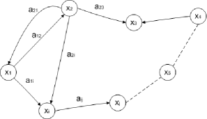
Figure 1.

This definition allows for some pairs of nodes to be disconnected if the corresponding element of the matrix $A$ is $\mathbf{0}$ and for some channels to be “loops” with coincident ends if the matrix $A$ has nonzero diagonal elements.

Recall that a sequence of nodes of the form

$$p=(y_{0},y_{1},\dots,y_{k})$$

with $k\geq 0$ and $(y_{i},y_{i+1})\in\Gamma$, $i=0,\dots,k-1$, is called a path of length $k$ connecting $y_{0}$ with $y_{k}$. Denote the set of all such paths by $P_{k}(y_{0},y_{k})$. The weight $A(p)$ of a path $p\in P_{k}(y_{0},y_{k})$ is defined to be the product of weights of arcs connecting consecutive nodes of the path:

$$A(p)=A(y_{0},y_{1})\odot\cdots\odot A(y_{k-1},y_{k}).$$

By definition, for a ‘path’ $p\in P_{0}(x_{i},x_{j})$ of length $k=0$ the weight is $\mathbf{1}$ if $i=j$ and $\mathbf{0}$ otherwise.

For each matrix $A\in\operatorname{Mat}_{nn}(S)$ define $A^{0}=E=(\delta_{ij})$ (where $\delta_{ij}=\mathbf{1}$ if $i=j$ and $\delta_{ij}=\mathbf{0}$ otherwise) and $A^{k}=AA^{k-1}$, $k\geq 1$. Let $a^{[k]}_{ij}$ be the $(i,j)$th element of the matrix $A^{k}$. It is easily checked that

$$a^{[k]}_{ij}=\bigoplus_{\begin{subarray}{c}i_{0}=i,\,i_{k}=j\\ 1\leq i_{1},\ldots,i_{k-1}\leq n\end{subarray}}a_{i_{0}i_{1}}\odot\dots\odot a_{i_{k-1}i_{k}}.$$

Thus $a^{[k]}_{ij}$ is the supremum of the set of weights corresponding to all paths of length $k$ connecting the node $x_{i_{0}}=x_{i}$ with $x_{i_{k}}=x_{j}$.

Let $A^{*}$ be defined as in (6). Denote the elements of the matrix $A^{*}$ by $a^{*}_{ij}$, $i,j=1,\dots,n$; then

$$a^{*}_{ij}=\bigoplus_{0\leq k<\infty}\bigoplus_{p\in P_{k}(x_{i},x_{j})}A(p).$$

The closure matrix $A^{*}$ solves the well-known algebraic path problem, which is formulated as follows: for each pair $(x_{i},x_{j})$ calculate the supremum of weights of all paths (of arbitrary length) connecting node $x_{i}$ with node $x_{j}$. The closure operation in matrix semirings has been studied extensively (see, for instance, [2, 7, 8, 10, 13, 16, 17, 20, 34] and references therein).

Example 1 (The shortest path problem).

Let $S=\mathbf{R}_{\min}$, so the weights are real numbers. In this case

$$A(p)=A(y_{0},y_{1})+A(y_{1},y_{2})+\dots+A(y_{k-1},y_{k}).$$

If the element $a_{ij}$ specifies the length of the arc $(x_{i},x_{j})$ in some metric, then $a^{*}_{ij}$ is the length of the shortest path connecting $x_{i}$ with $x_{j}$.

Example 2 (The maximal path width problem).

Let $S=\mathbf{R}\cup\{\mathbf{0},\mathbf{1}\}$ with $\oplus=\max$, $\odot=\min$. Then

$$a^{*}_{ij}=\max_{p\in\bigcup\limits_{k\geq 1}P_{k}(x_{i},x_{j})}A(p),$$

$$A(p)=\min(A(y_{0},y_{1}),\dots,A(y_{k-1},y_{k})).$$

If the element $a_{ij}$ specifies the “width” of the arc $(x_{i},x_{j})$, then the width of a path $p$ is defined as the minimal width of its constituting arcs and the element $a^{*}_{ij}$ gives the supremum of possible widths of all paths connecting $x_{i}$ with $x_{j}$.

Example 3 (A simple dynamic programming problem).

Let $S=\mathbf{R}_{\max}$ and suppose $a_{ij}$ gives the profit corresponding to the transition from $x_{i}$ to $x_{j}$. Define the vector $B=(b_{i})\in\operatorname{Mat}_{n1}(\mathbf{R}_{\max})$ whose element $b_{i}$ gives the terminal profit corresponding to exiting from the graph through the node $x_{i}$. Of course, negative profits (or, rather, losses) are allowed. Let $m$ be the total profit corresponding to a path $p\in P_{k}(x_{i},x_{j})$, that is

$$m=A(p)+b_{j}.$$

Then it is easy to check that the supremum of profits that can be achieved on paths of length $k$ beginning at the node $x_{i}$ is equal to $(A^{k}B)_{i}$ and the supremum of profits achievable without a restriction on the length of a path equals $(A^{*}B)_{i}$.

Example 4 (The matrix inversion problem).

Note that in the formulas of this section we are using distributivity of the multiplication $\odot$ with respect to the addition $\oplus$ but do not use the idempotency axiom. Thus the algebraic path problem can be posed for a nonidempotent semiring $S$ as well (see, for instance, [45]). For instance, if $S=\mathbf{R}$, then

$$A^{*}=I+A+A^{2}+\dotsb=(I-A)^{-1}.$$

If $\|A\|>1$ but the matrix $I-A$ is invertible, then this expression defines a regularized sum of the divergent matrix power series $\sum_{i\geq 0}A^{i}$.

We emphasize that this connection between the matrix closure operation and solutions to the Bellman equation gives rise to a number of different algorithms for numerical calculation of the matrix closure. All these algorithms are adaptations of the well-known algorithms of the traditional computational linear algebra, such as the Gauss–Jordan elimination, various iterative and escalator schemes, etc. This is a special case of the idempotent superposition principle (see below).

2.4. Interval analysis over positive semirings

Traditional interval analysis is a nontrivial and popular mathematical area, see, for instance, [1, 12, 21, 40, 43]. An “idempotent” version of interval analysis (and moreover interval analysis over positive semirings) appeared in [33, 34, 49]. Rather many publications on the subject appeared later, see, for instance, [9, 12, 19, 41, 42]. Interval analysis over the positive semiring $\textbf{R}_{+}$ was discussed in [4].

Let a set $S$ be partially ordered by a relation $\preceq$. A closed interval in $S$ is a subset of the form $\mathbf{x}=[\underline{\mathbf{x}},\overline{\mathbf{x}}]=\{\,x\in S\mid\underline{\mathbf{x}}\preceq x\preceq\overline{\mathbf{x}}\,\}$, where the elements $\underline{\mathbf{x}}\preceq\overline{\mathbf{x}}$ are called lower and upper bounds of the interval $\mathbf{x}$. The order $\preceq$ induces a partial ordering on the set of all closed intervals in $S$: $\mathbf{x}\preceq\mathbf{y}$ iff $\underline{\mathbf{x}}\preceq\underline{\mathbf{y}}$ and $\overline{\mathbf{x}}\preceq\overline{\mathbf{y}}$.

A weak interval extension $I(S)$ of a positive semiring $S$ is the set of all closed intervals in $S$ endowed with operations $\oplus$ and $\odot$ defined as ${\mathbf{x}\oplus\mathbf{y}}=[{\underline{\mathbf{x}}\oplus\underline{\mathbf{y}}},{\overline{\mathbf{x}}\oplus\overline{\mathbf{y}}}]$, ${\mathbf{x}\odot\mathbf{y}}=[{\underline{\mathbf{x}}\odot\underline{\mathbf{y}}},{\overline{\mathbf{x}}\odot\overline{\mathbf{y}}}]$ and a partial order induced by the order in $S$. The closure operation in $I(S)$ is defined by $\mathbf{x}^{*}=[\underline{\mathbf{x}}^{*},\overline{\mathbf{x}}^{*}]$. There are some other interval extensions (including the so-called strong interval extension [34]) but the weak extension is more convenient.

The extension $I(S)$ is positive; $I(S)$ is idempotent if $S$ is an idempotent semiring. A universal algorithm over $S$ can be applied to $I(S)$ and we shall get an interval version of the initial algorithm. Usually both versions have the same complexity. For the discrete stationary Bellman equation and the corresponding optimization problems on graphs, interval analysis was examined in [33, 34] in details. Other problems of idempotent linear algebra were examined in [9, 12, 19, 41, 42].

Idempotent mathematics appears to be remarkably simpler than its traditional analog. For example, in traditional interval arithmetic, multiplication of intervals is not distributive with respect to addition of intervals, whereas in idempotent interval arithmetic this distributivity is preserved. Moreover, in traditional interval analysis the set of all square interval matrices of a given order does not form even a semigroup with respect to matrix multiplication: this operation is not associative since distributivity is lost in the traditional interval arithmetic. On the contrary, in the idempotent (and positive) case associativity is preserved. Finally, in traditional interval analysis some problems of linear algebra, such as solution of a linear system of interval equations, can be very difficult (more precisely, they are $NP$-hard, see  [21] and references therein). It was noticed in [33, 34] that in the idempotent case solving an interval linear system requires a polynomial number of operations (similarly to the usual Gauss elimination algorithm). Two properties that make the idempotent interval arithmetic so simple are monotonicity of arithmetic operations and positivity of all elements of an idempotent semiring.

Interval estimates in idempotent mathematics are usually exact. In the traditional theory such estimates tend to be overly pessimistic.

2.5. Idempotent correspondence principle

There is a nontrivial analogy between mathematics of semirings and quantum mechanics. For example, the field of real numbers can be treated as a “quantum object” with respect to idempotent semirings. So idempotent semirings can be treated as “classical” or “semi-classical” objects with respect to the field of real numbers.

Let $\mathbf{R}$ be the field of real numbers and $\mathbf{R}_{+}$ the subset of all non-negative numbers. Consider the following change of variables:

$$u\mapsto w=h\ln u,$$

where $u\in\mathbf{R}_{+}\setminus\{0\}$, $h>0$; thus $u=e^{w/h}$, $w\in\mathbf{R}$. Denote by $\mathbf{0}$ the additional element $-\infty$ and by $S$ the extended real line $\mathbf{R}\cup\{\mathbf{0}\}$. The above change of variables has a natural extension $D_{h}$ to the whole $S$ by $D_{h}(0)=\mathbf{0}$; also, we denote $D_{h}(1)=0=\mathbf{1}$.

Denote by $S_{h}$ the set $S$ equipped with the two operations $\oplus_{h}$ (generalized addition) and $\odot_{h}$ (generalized multiplication) such that $D_{h}$ is a homomorphism of $\{\mathbf{R}_{+},+,\cdot\}$ to $\{S,\oplus_{h},\odot_{h}\}$. This means that $D_{h}(u_{1}+u_{2})=D_{h}(u_{1})\oplus_{h}D_{h}(u_{2})$ and $D_{h}(u_{1}\cdot u_{2})=D_{h}(u_{1})\odot_{h}D_{h}(u_{2})$, that is, $w_{1}\odot_{h}w_{2}=w_{1}+w_{2}$ and $w_{1}\oplus_{h}w_{2}=h\ln(e^{w_{1}/h}+e^{w_{2}/h})$. It is easy to prove that $w_{1}\oplus_{h}w_{2}\to\max\{w_{1},w_{2}\}$ as $h\to 0$.

$\mathbf{R}_{+}$ and $S_{h}$ are isomorphic semirings; therefore we have obtained $\mathbf{R}_{\max}$ as a result of a deformation of $\mathbf{R}_{+}$. We stress the obvious analogy with the quantization procedure, where $h$ is the analog of the Planck constant. In these terms, $\mathbf{R}_{+}$ (or $\mathbf{R}$) plays the part of a “quantum object” while $\mathbf{R}_{\max}$ acts as a “classical” or “semi-classical” object that arises as the result of a dequantization of this quantum object. In the case of $\mathbf{R}_{\min}$, the corresponding dequantization procedure is generated by the change of variables $u\mapsto w=-h\ln u$.

There is a natural transition from the field of real numbers or complex numbers to the idempotent semiring $\mathbf{R}_{\max}$ (or $\mathbf{R}_{\min}$). This is a composition of the mapping $x\mapsto|x|$ and the deformation described above.

In general an idempotent dequantization is a transition from a basic field to an idempotent semiring in mathematical concepts, constructions and results, see [24, 26] for details. Idempotent dequantization suggests the following formulation of the idempotent correspondence principle:

There exists a heuristic correspondence between interesting, useful, and important constructions and results over the field of real (or complex) numbers and similar constructions and results over idempotent semirings in the spirit of N. Bohr’s correspondence principle in quantum mechanics.

Thus idempotent mathematics can be treated as a “classical shadow (or counterpart)” of the traditional Mathematics over fields. A systematic application of this correspondence principle leads to a variety of theoretical and applied results, see, for instance,  [24, 26, 30, 34, 39, 52, 53]. Relations to quantum physics are discussed in detail, for instance, in [24].

In this paper we aim to develop a practical systematic application of the correspondence principle to the algorithms of linear algebra and discrete mathematics. For the remainder of this subsection let us focus on an idea how the idempotent correspondence principle may lead to a unifying approach to hardware design. (See [35, 28] for more information.)

The most important and standard numerical algorithms have many hardware realizations in the form of technical devices or special processors. These devices often can be used as prototypes for new hardware units resulting from mere substitution of the usual arithmetic operations by their semiring analogs (and additional tools for generating neutral elements $\mathbf{0}$ and $\mathbf{1}$). Of course, the case of numerical semirings consisting of real numbers (maybe except neutral elements) and semirings of numerical intervals is the most simple and natural. Note that for semifields (including $\mathbf{R}_{\max}$ and $\mathbf{R}_{\min}$) the operation of division is also defined.

Good and efficient technical ideas and decisions can be taken from prototypes to new hardware units. Thus the correspondence principle generates a regular heuristic method for hardware design. Note that to get a patent it is necessary to present the so-called ‘invention formula’, that is to indicate a prototype for the suggested device and the difference between these devices.

Consider (as a typical example) the most popular and important algorithm of computing the scalar product of two vectors:

(9) $$(x,y)=x_{1}y_{1}+x_{2}y_{2}+\cdots+x_{n}y_{n}.$$

The universal version of (9) for any semiring $A$ is obvious:

(10) $$(x,y)=(x_{1}\odot y_{1})\oplus(x_{2}\odot y_{2})\oplus\cdots\oplus(x_{n}\odot y_{n}).$$

In the case $A=\mathbf{R}_{\max}$ this formula turns into the following one:

(11) $$(x,y)=\max\{x_{1}+y_{1},x_{2}+y_{2},\cdots,x_{n}+y_{n}\}.$$

This calculation is standard for many optimization algorithms, so it is useful to construct a hardware unit for computing (11). There are many different devices (and patents) for computing (9) and every such device can be used as a prototype to construct a new device for computing (11) and even (10). Many processors for matrix multiplication and for other algorithms of linear algebra are based on computing scalar products and on the corresponding “elementary” devices. Using modern technologies it is possible to construct cheap special-purpose multi-processor chips and systolic arrays of elementary processors implementing universal algorithms. See, for instance,  [35, 28, 45] where the systolic arrays and parallel computing issues are discussed for the algebraic path problem. In particular, there is a systolic array of $n(n+1)$ elementary processors which performs computations of the Gauss–Jordan elimination algorithm and can solve the algebraic path problem within $5n-2$ time steps.

3. Some universal algorithms of linear algebra

In this section we discuss universal algorithms computing $A^{*}$ and $A^{*}B$. We start with the basic escalator and Gauss-Jordan elimination techniques in Subsect. 3.1 and continue with its specification to the case of Toeplitz systems in Subsect. 3.2. The universal LDM decomposition of Bellman equations is explained in Subsect. 3.3, followed by its adaptations to symmetric and band matrices in Subsect. 3.4. The iteration schemes are discussed in Subsect. 3.5. In the final Subsect. 3.6 we discuss the implementations of universal algorithms.

Algorithms themselves will be described in a language of Matlab, following the tradition of Golub and van Loan [14]. This is done for two purposes: 1) to simplify the comparison of the algorithms with their prototypes taken mostly from [14], 2) since the language of Matlab is designed for matrix computations. We will not formally describe the rules of our Matlab-derived language, preferring just to outline the following important features:

• Our basic arithmetic operations are $a\oplus b$, $a\odot b$ and $a^{*}$.

• The vectorization of these operations follows the rules of Matlab.

• We use basic keywords of Matlab like ‘for’, ‘while’, ’if’ and ’end’, similar to other programming languages like $C++$ or Java.

Let us give some examples of universal matrix computations in our language:
Example 1. $v(1:j)=\alpha^{*}\odot a(1:j,k)$ means that the result of (scalar) multiplication of the first $j$ components of the $k$th column of $A$ by the closure of $\alpha$ is assigned to the first $j$ components of $v$.
Example 2. $a(i,j)=a(i,j)\oplus a(i,1:n)\odot a(1:n,j)$ means that we add ($\oplus$) to the entry $a_{ij}$ of $A$ the result of the (universal) scalar multiplication of the $i$th row with the $j$th column of $A$ (assumed that $A$ is $n\times n$).
Example 3. $a(1:n,k)\odot b(l,1:m)$ means the outer product of the $k$th column of $A$ with the $l$th row of $B$. The entries of resulting matrix $C=(c_{ij})$ equal $c_{ij}=a_{ik}\odot b_{lj}$, for all $i=1,\ldots,n$ and $j=1,\ldots,m$.
Example 4. $x(1:n)\odot y(n:-1:1)$ is the scalar product of vector $x$ with vector $y$ whose components are taken in the reverse order: the proper algebraic expression is $\bigoplus_{i=1}^{n}x_{i}\odot y_{n+1-i}$.
Example 5. The following cycle yields the same result as in the previous example: $s=0$
for $i=1:n$
$s=s\oplus x(i)\odot x(n+1-i)$
end

3.1. Escalator scheme and Gauss-Jordan elimination

We first analyse the basic escalator method, based on the definition of matrix closures (4). Let $A$ be a square matrix. Closures of its main submatrices $A_{k}$ can be found inductively, starting from $A_{1}^{*}=(a_{11})^{*}$, the closure of the first diagonal entry. Generally we represent $A_{k+1}$ as

$$A_{k+1}=\begin{pmatrix}A_{k}&g_{k}\\ h_{k}^{T}&a_{k+1}\end{pmatrix},$$

assuming that we have found the closure of $A_{k}$. In this representation, $g_{k}$ and $h_{k}$ are columns with $k$ entries and $a_{k+1}$ is a scalar. We also represent $A_{k+1}^{*}$ as

$$A_{k+1}^{*}=\begin{pmatrix}U_{k}&v_{k}\\ w_{k}^{T}&u_{k+1}\end{pmatrix}.$$

Using (4) we obtain that

(12) $$\begin{split}u_{k+1}&=(h_{k}^{T}A_{k}^{*}g_{k}\oplus a_{k+1})^{*},\\ v_{k}&=A_{k}^{*}g_{k}u_{k+1},\\ w_{k}^{T}&=u_{k+1}h_{k}^{T}A_{k}^{*},\\ U_{k}&=A_{k}^{*}g_{k}u_{k+1}h_{k}^{T}A_{k}^{*}\oplus A_{k}^{*}.\end{split}$$

An algorithm based on (12) can be written as follows.

Algorithm 1.

Escalator method for computing $A^{*}$

Input: an $n\times n$ matrix $A$ with entries $a(i,j)$,
also used to store the final result
and the intermediate results of the computation process.

$a(1,1)=(a(1,1))^{*}$
for $i=1:n-1$
$Ag=a(1:i,1:i)\odot a(1:i,i+1)$
$hA=a(i+1,1:i)\odot a(1:i,1:i)$
$a(i+1,i+1)=a(i+1,i+1)\oplus a(i+1,1:i)\odot Ag(1:i,1)$
$a(i+1,i+1)=(a(i+1,i+1))^{*}$
$a(1:i,i+1)=a(i+1,i+1)\odot Ag$
$a(i+1,1:i)=a(i+1,i+1)\odot hA$
$a(1:i,1:i)=a(1:i,1:i)\oplus Ag\odot a(i+1,i+1)\odot hA$
end

In full analogy with its linear algebraic prototype, the algorithm requires $n^{3}+O(n^{2})$ operations of addition $\oplus$, $n^{3}+O(n^{2})$ operations of multiplication $\odot$, and $n$ operations of taking algebraic closure. The linear-algebraic prototype of the method written above is also called the bordering method in the literature [7, 11].

Alternatively, we can obtain a solution of $X=AX\oplus B$ as a result of elimination process, whose informal explanation is given below. If $A^{*}$ is defined as $\bigoplus_{i\geq 0}A^{i}$ (including the scalar case), then $A^{*}B$ is the least solution of $X=AX\oplus B$ for all $A$ and $B$ of appropriate sizes. In this case, the solution found by the elimination process given below coincides with $A^{*}B$.

For matrix $A=(a_{ij})$ and column vectors $x=(x_{i})$ and $b=(b_{i})$ (restricting without loss of generality to the column vectors), the Bellman equation $x=Ax\oplus b$ can be written as

$$\begin{pmatrix}x_{1}\\ x_{2}\\ \vdots\\ x_{n}\end{pmatrix}=\begin{pmatrix}a_{11}&a_{12}&\ldots&a_{1n}\\ a_{21}&a_{22}&\ldots&a_{2n}\\ \vdots&\vdots&\ddots&\vdots\\ a_{n1}&a_{n2}&\ldots&a_{nn}\end{pmatrix}\begin{pmatrix}x_{1}\\ x_{2}\\ \vdots\\ x_{n}\end{pmatrix}\oplus$$

(13) $$\begin{pmatrix}\mathbf{1}&\mathbf{0}&\ldots&\mathbf{0}\\ \mathbf{0}&\mathbf{1}&\ldots&\mathbf{0}\\ \vdots&\vdots&\ddots&\vdots\\ \mathbf{0}&\mathbf{0}&\ldots&\mathbf{1}\end{pmatrix}\begin{pmatrix}b_{1}\\ b_{2}\\ \vdots\\ b_{n}\end{pmatrix}.$$

After expressing $x_{1}$ in terms of $x_{2},\ldots,x_{n}$ from the first equation and substituting this expression for $x_{1}$ in all other equations from the second to the $n$th we obtain

$$\begin{pmatrix}x_{1}\\ x_{2}\\ \vdots\\ x_{n}\end{pmatrix}=$$

$$\begin{pmatrix}\mathbf{0}&(a_{11})^{*}a_{12}&\ldots&(a_{11})^{*}a_{1n}\\ \mathbf{0}&a_{22}\oplus(a_{21}(a_{11})^{*}a_{12})&\ldots&a_{2n}\oplus(a_{21}(a_{11})^{*}a_{1n})\\ \vdots&\vdots&\ddots&\vdots\\ \mathbf{0}&a_{n2}\oplus(a_{n1}(a_{11})^{*}a_{12})&\ldots&a_{nn}\oplus(a_{n1}(a_{11})^{*}a_{1n})\end{pmatrix}$$

(14) $$\begin{pmatrix}x_{1}\\ x_{2}\\ \vdots\\ x_{n}\end{pmatrix}\oplus\begin{pmatrix}(a_{11})^{*}&\mathbf{0}&\ldots&\mathbf{0}\\ a_{21}(a_{11})^{*}&\mathbf{1}&\ldots&\mathbf{0}\\ \vdots&\vdots&\ddots&\vdots\\ a_{n1}(a_{11})^{*}&\mathbf{0}&\ldots&\mathbf{1}\end{pmatrix}\begin{pmatrix}b_{1}\\ b_{2}\\ \vdots\\ b_{n}\end{pmatrix}$$

Note that nontrivial entries in both matrices occupy complementary places, so during computations both matrices can be stored in the same square array $C^{(k)}$. Denote its elements by $c^{(k)}_{ij}$ where $k$ is the number of eliminated variables. After $l-1$ eliminations we have

(15) $$\begin{split}x_{l}&=(c_{ll}^{(l-1)})^{*}b_{l},\\ c_{il}^{(l)}&=c_{il}^{(l-1)}(c_{ll}^{(l-1)})^{*},\quad i=1,\ldots,l-1,l+1,\ldots,n\\ c_{ij}^{(l)}&=c_{ij}^{(l-1)}\oplus c_{il}^{(l-1)}(c_{ll}^{(l-1)})^{*}c_{lj}^{(l-1)},\\ i,j&=1,\ldots,l-1,l+1,\ldots,n\\ c_{li}^{(l)}&=(c_{ll}^{(l-1)})^{*}c_{li}^{(l-1)},\quad i=1,\ldots,l-1,l+1,\ldots,n\\ \end{split}$$

After $n$ eliminations we get $x=C^{(n)}b$. Taking as $b$ any vector with one coordinate equal to $\mathbf{1}$ and the rest equal to $\mathbf{0}$, we obtain $C^{(n)}=A^{*}$. We write out the following algorithm based on recursion (15).

Algorithm 2.

Gauss-Jordan elimination for computing $A^{*}$.

Input: an $n\times n$ matrix $A$ with entries $a(i,j)$,
also used to store the final result
and intermediate results of the computation process.

for $i=1:n$
$a(i,i)=(a(i,i))^{*}$
for $k=1:n$
if $k\neq i$
$a(k,i)=a(k,i)\odot a(i,i)$
end
end
for $k=1:n$
for $j=1:n$
if $k\neq i\ \&\ j\neq i$
$a(k,j)=a(k,j)\oplus a(k,i)\odot a(i,j)$
end
end
for $j=1:n$
if $j\neq i$
$a(i,j)=a(i,i)\odot a(i,j)$
end
end
end

Remark 1.

Algorithm 2 can be regarded as a “universal Floyd-Warshall algorithm” generalizing the well-known algorithms of Warshall and Floyd for computing the transitive closure of a graph and all optimal paths on a graph. See, for instance, [46] for the description of these classical methods of discrete mathematics. In turn, these methods can be regarded as specifications of Algorithm 2 to the cases of max-plus and Boolean semiring.

Remark 2.

Algorithm 2 is also close to Yershov’s “refilling” method for inverting matrices and solving systems $Ax=b$ in the classical linear algebra, see [11] Chapter 2 for details.

3.2. Toeplitz systems

We start by considering the escalator method for finding the solution $x=A^{*}b$ to  $x=Ax\oplus b$, where $x$ and $b$ are column vectors. Firstly, we have $x^{(1)}=A_{1}^{*}b_{1}$. Let $x^{(k)}$ be the vector found after $(k-1)$ steps, and let us write

$$x^{(k+1)}=\begin{pmatrix}z\\ x_{k+1}\end{pmatrix}.$$

Using (12) we obtain that

(16) $$\begin{split}x_{k+1}=u_{k+1}(h_{k}^{T}x^{(k)}\oplus b_{k+1}),\\ z=x^{(k)}\oplus A_{k}^{*}g_{k}x_{k+1}.\end{split}$$

We have to compute $A_{k}^{*}g_{k}$. In general, we would have to use Algorithm 1. Next we show that this calculation can be done very efficiently when $A$ is symmetric Toeplitz.

Formally, a matrix $A\in\operatorname{Mat}_{nn}({\mathcal{S}})$ is called Toeplitz if there exist scalars $r_{-n+1},\ldots,r_{0},\ldots,r_{n-1}$ such that $A_{ij}=r_{j-i}$ for all $i$ and $j$. Informally, Toeplitz matrices are such that their entries are constant along any line parallel to the main diagonal (and along the main diagonal itself). For example,

$$A=\begin{pmatrix}r_{0}&r_{1}&r_{2}&r_{3}\\ r_{-1}&r_{0}&r_{1}&r_{2}\\ r_{-2}&r_{-1}&r_{0}&r_{1}\\ r_{-3}&r_{-2}&r_{-1}&r_{0}\end{pmatrix}$$

is Toeplitz. Such matrices are not necessarily symmetric. However, they are always persymmetric, that is, symmetric with respect to the inverse diagonal. This property is algebraically expressed as $A=E_{n}A^{T}E_{n}$, where $E_{n}=[e_{n},\ldots,e_{1}]$. By $e_{i}$ we denote the column whose $i$th entry is ${\mathbf{1}}$ and other entries are $O$. The property $E_{n}^{2}=I_{n}$ (where $I_{n}$ is the $n\times n$ identity matrix) implies that the product of two persymmetric matrices is persymmetric. Hence any degree of a persymmetric matrix is persymmetric, and so is the closure of a persymmetric matrix. Thus, if $A$ is persymmetric, then

(17) $$E_{n}A^{*}=(A^{*})^{T}E_{n}.$$

Further we deal only with symmetric Toeplitz matrices. Consider the equation $y=T_{n}y\oplus r^{(n)}$, where $r^{(n)}=(r_{1},\ldots,r_{n})^{T}$, and $T_{n}$ is defined by the scalars $r_{0},r_{1},\ldots,r_{n-1}$ so that $T_{ij}=r_{|j-i|}$ for all $i$ and $j$. This is a generalization of the Yule-Walker problem [14]. Assume that we have obtained the least solution $y^{(k)}$ to the system $y=T_{k}y\oplus r^{(k)}$ for some $k$ such that $1\leq k\leq n-1$, where $T_{k}$ is the main $k\times k$ submatrix of $T_{n}$. We write $T_{k+1}$ as

$$T_{k+1}=\begin{pmatrix}T_{k}&E_{k}r^{(k)}\\ r^{(k)T}E_{k}&r_{0}\end{pmatrix}.$$

We also write $y^{(k+1)}$ and $r^{(k+1)}$ as

$$y^{(k+1)}=\begin{pmatrix}z\\ \alpha_{k}\end{pmatrix},\quad r^{(k+1)}=\begin{pmatrix}r^{(k)}\\ r_{k+1}\end{pmatrix}.$$

Using (16), (17) and the identity $T_{k}^{*}r^{(k)}=y^{(k)}$, we obtain that

$$\begin{split}\alpha_{k}&=(r_{0}\oplus r^{(k)T}y^{(k)})^{*}(r^{(k)T}E_{k}y^{(k)}\oplus r_{k+1}),\\ z&=E_{k}y^{(k)}\alpha_{k}\oplus y^{(k)}.\end{split}$$

Denote $\beta_{k}=r_{0}\oplus r^{(k)T}y^{(k)}$. The following argument shows that $\beta_{k}$ can be found recursively if $(\beta_{k-1}^{*})^{-1}$ exists.

$$\begin{split}\beta_{k}&=r_{0}\oplus[r^{(k-1)T}\ r_{k}]\begin{pmatrix}E_{k-1}y^{(k-1)}\alpha_{k-1}\oplus y^{(k-1)}\\ \alpha_{k-1}\end{pmatrix}\\ &=r_{0}\oplus r^{(k-1)T}y^{(k-1)}\oplus(r^{(k-1)T}E_{k-1}y^{(k-1)}\oplus\end{split}$$

(18) $$r_{k})\alpha_{k-1}=\beta_{k-1}\oplus(\beta_{k-1}^{*})^{-1}\odot\alpha_{k-1}^{2}.$$

Existence of $(\beta_{k-1}^{*})^{-1}$ is not universal, and this will make us write two versions of our algorithm, the first one involving (18), and the second one not involving it. We will write these two versions in one program and mark the expressions which refer only to the first version or to the second one by the MATLAB-style comments $\%1$ and $\%2$, respectively. Collecting the expressions for $\beta_{k}$, $\alpha_{k}$ and $z$ we obtain the following recursive expression for $y^{(k)}$:

(19) $$\begin{split}\beta_{k}&=r_{0}\oplus r^{(k)T}y^{(k)},\qquad\%2\\ \beta_{k}&=\beta_{k-1}\oplus(\beta_{k-1}^{*})^{-1}\odot\alpha_{k-1}^{2},\qquad\%1\\ \alpha_{k}&=(\beta_{k})^{*}\odot(r^{(k)T}E_{k}y^{(k)}\oplus r_{k+1}),\\ y^{(k+1)}&=\begin{pmatrix}E_{k}y^{(k)}\alpha_{k}\oplus y^{(k)}\\ \alpha_{k}\end{pmatrix}.\end{split}$$

Recursive expression (19) is a generalized version of the Durbin method for the Yule-Walker problem, see [14] Algorithm 4.7.1 for a prototype.

Algorithm 3.

The Yule-Walker problem for the Bellman equations with symmetric Toeplitz matrix.

Input: $r_{0}$: scalar,
$r$: $n-1\times 1$ vector;

$y(1)=r_{0}^{*}\odot r(1)$
$\beta=r_{0}\qquad\%1$
$\alpha=r_{0}^{*}\odot r(1)$
for $k=1:n-1$
$\beta=r_{0}\oplus r(1:k)\odot y(1:k)\qquad\%2$
$\beta=\beta\oplus(\beta^{*})^{-1}\odot\alpha^{2}\qquad\%1$
$\alpha=\beta^{*}\odot(r(k:-1:1)\odot y(1:k)\oplus r(k+1))$
$z(1:k)=y(1:k)\oplus y(k:-1:1)\odot\alpha$
$y(1:k)=z(1:k)$
$y(k+1)=\alpha$
end

Output: vector $y$.

In the general case, the algorithm requires $3/2n^{2}+O(n)$ operations $\oplus$ and $\odot$ each, and just $n^{2}+O(n)$ of $\oplus$ and $\odot$ if inversions of algebraic closures are allowed (as usual, just $n$ such closures are required in both cases).

Now we consider the problem of finding $x^{(n)}=T_{n}^{*}b^{(n)}$ where $T_{n}$ is as above and $b^{(n)}=(b_{1},\ldots,b_{n})$ is arbitrary. We also introduce the column vectors $y^{(k)}$ which solve the Yule-Walker problem: $y^{(k)}=T_{k}^{*}r^{(k)}$. The main idea is to find the expression for $x^{(k+1)}=T_{k+1}^{*}b^{(k+1)}$ involving $x^{(k)}$ and $y^{(k)}$. We write $x^{(k+1)}$ and $b^{(k+1)}$ as

$$x^{(k+1)}=\begin{pmatrix}v\\ \mu_{k}\end{pmatrix},\quad b^{(k+1)}=\begin{pmatrix}b^{(k)}\\ b_{k+1}\end{pmatrix}.$$

Making use of the persymmetry of $T_{k}^{*}$ and of the identities $T_{k}^{*}b_{k}=x^{(k)}$ and $T_{k}^{*}r_{k}=y^{(k)}$, we specialize expressions (16) and obtain that

$$\begin{split}\mu_{k}&=(r_{0}\oplus r^{(k)T}y^{(k)})^{*}\odot(r^{(k)T}E_{k}x^{(k)}\oplus b_{k+1}),\\ v&=E_{k}y^{(k)}\mu_{k}\oplus x^{(k)}.\end{split}$$

The coefficient $r_{0}\oplus r^{(k)T}y^{(k)}=\beta_{k}$ can be expressed again as $\beta_{k}=\beta_{k-1}\oplus(\beta_{k-1}^{*})^{-1}\odot(\alpha_{k-1})^{2}$, if the closure $(\beta_{k-1})^{*}$ is invertible. Using this we obtain the following recursive expression:

(20) $$\begin{split}\beta_{k}&=r_{0}\oplus r^{(k)T}y^{(k)},\qquad\%2\\ \beta_{k}&=\beta_{k-1}\oplus(\beta_{k-1}^{*})^{-1}\odot\alpha_{k-1}^{2},\qquad\%1\\ \mu_{k}&=\beta_{k}^{*}\odot(r^{(k)T}E_{k}x^{(k)}\oplus b_{k+1}),\\ x^{(k+1)}&=\begin{pmatrix}E_{k}y^{(k)}\mu_{k}\oplus x^{(k)}\\ \mu_{k}\end{pmatrix}.\end{split}$$

Expressions (19) and (20) yield the following generalized version of the Levinson algorithm for solving linear symmetric Toeplitz systems, see [14] Algorithm 4.7.2 for a prototype:

Algorithm 4.

Bellman system with symmetric Toeplitz matrix

Input: $r_{0}$: scalar,
$r$: $1\times n-1$ row vector;
$b$: $n\times 1$ column vector.

$y(1)=r_{0}^{*}\odot r(1)$; $x(1)=r_{0}^{*}\odot b(1)$;
$\beta=r_{0}\qquad\%1$
$\alpha=r_{0}^{*}\odot r(1)$
for $k=1:n-1$
$\beta=r_{0}\oplus r(1:k)\odot y(1:k)\qquad\%2$
$\beta=\beta\oplus(\beta^{*})^{-1}\odot\alpha^{2}\qquad\%1$
$\mu=\beta^{*}\odot(r(k:-1:1)\odot x(1:k)\oplus b(k+1))$
$v(1:k)=x(1:k)\oplus y(k:-1:1)\odot\mu$
$x(1:k)=v(1:k)$
$x(k+1)=\mu$
if $k<n-1$
$\alpha=\beta^{*}\odot(r(k:-1:1)\odot y(1:k)\oplus r(k+1))$
$z(1:k)=y(1:k)\oplus y(k:-1:1)\odot\alpha$
$y(1:k)=z(1:k)$
$y(k+1)=\alpha$
end
end

Output: vector $x$.

In the general case, the algorithm requires $5/2n^{2}+O(n)$ operations $\oplus$ and $\odot$ each, and just $2n^{2}+O(n)$ of $\oplus$ and $\odot$ if inversions of algebraic closures are allowed (as usual, just $n$ such closures are required in both cases).

3.3. LDM decomposition

Factorization of a matrix into the product $A=LDM$, where $L$ and $M$ are lower and upper triangular matrices with a unit diagonal, respectively, and $D$ is a diagonal matrix, is used for solving matrix equations $AX=B$. We construct a similar decomposition for the Bellman equation $X=AX\oplus B$.

For the case $AX=B$, the decomposition $A=LDM$ induces the following decomposition of the initial equation:

(21) $$LZ=B,\qquad DY=Z,\qquad MX=Y.$$

Hence, we have

(22) $$A^{-1}=M^{-1}D^{-1}L^{-1},$$

if $A$ is invertible. In essence, it is sufficient to find the matrices $L$, $D$ and $M$, since the linear system $AX=B$ is easily solved by a combination of the forward substitution for $Z$, the trivial inversion of a diagonal matrix for $Y$, and the back substitution for $X$.

Using the LDM-factorization of $AX=B$ as a prototype, we can write

(23) $$Z=LZ\oplus B,\qquad Y=DY\oplus Z,\qquad X=MX\oplus Y.$$

Then

(24) $$A^{*}=M^{*}D^{*}L^{*}.$$

A triple $(L,D,M)$ consisting of a lower triangular, diagonal, and upper triangular matrices is called an $LDM$-factorization of a matrix $A$ if relations (23) and (24) are satisfied. We note that in this case, the principal diagonals of $L$ and $M$ are zero.

Our universal modification of the $LDM$-factorization used in matrix analysis for the equation $AX=B$ is similar to the $LU$-factorization of Bellman equation suggested by Carré in [7, 8].

If $A$ is a symmetric matrix over a semiring with a commutative multiplication, the amount of computations can be halved, since $M$ and $L$ are mapped into each other under transposition.

We begin with the case of a triangular matrix $A=L$ (or $A=M$). Then, finding $X$ is reduced to the forward (or back) substitution. Note that in this case, equation $X=AX\oplus B$ has unique solution, which can be found by the obvious algorithms given below. In these algorithms $B$ is a vector (denoted by $b$), however they could be modified to the case when $B$ is a matrix of any appropriate size. We are interested only in the case of strictly lower-triangular, resp. strictly upper-triangular matrices, when $a_{ij}=0$ for $i\leq j$, resp. $a_{ij}=0$ for $i\geq j$.

Algorithm 5.

Forward substitution.

Input: Strictly lower-triangular $n\times n$ matrix $l$;
$n\times 1$ vector $b$.

for $k=2:n$
$y(k)=l(k,1:k-1)\odot y(1:k-1)$
end

Output: vector $y$.

Algorithm 6.

Backward substitution.

Input: Strictly upper-triangular $n\times n$ matrix $m$;
$n\times 1$ vector $b$.

for $k=n-1:-1:1$
$y(k)=m(k,k+1:n)\odot y(k+1:n)$
end

Output: vector $y$.

Both algorithms require $n^{2}/2+O(n)$ operations $\oplus$ and $\odot$, and no algebraic closures.

After performing a LDM-decomposition we also need to compute the closure of a diagonal matrix: this is done entrywise.

We now proceed with the algorithm of LDM decomposition itself, that is, computing matrices $L$, $D$ and $M$ satisfying (23) and (24). First we give an algorithm, and then we proceed with its explanation.

Algorithm 7.

LDM-decomposition (version 1).

Input: an $n\times n$ matrix $A$ with entries $a(i,j)$,
also used to store the final result
and intermediate results of the computation process.

for $j=1:n-1$
$v(j)=(a(j,j))^{*}$
$a(j+1:n,j)=a(j+1:n,j)\odot v(j)$
$a(j+1:n,j+1:n)=a(j+1:n,j+1:n)\oplus a(j+1:n,j)\odot a(j,j+1:n)$
$a(j,j+1:n)=v(j)\odot a(j,j+1:n)$
end

The algorithm requires $n^{3}/3+O(n^{2})$ operations $\oplus$ and $\odot$, and $n-1$ operations of algebraic closure.

The strictly triangular matrix $L$ is written in the lower triangle, the strictly upper triangular matrix $M$ in the upper triangle, and the diagonal matrix $D$ on the diagonal of the matrix computed by Algorithm 7. We now show that $A^{*}=M^{*}D^{*}L^{*}$. Our argument is close to that of [3].

We begin by representing, in analogy with the escalator method,

(25) $$A=\begin{pmatrix}a_{11}&h^{(1)}\\ g^{(1)}&B^{(1)}\end{pmatrix}$$

It can be verified that

$$A^{*}=\begin{pmatrix}{\mathbf{1}}&h^{(1)}a_{11}^{*}\\ O_{n-1\times 1}&I_{n-1}\end{pmatrix}\odot$$

(26) $$\begin{pmatrix}a_{11}^{*}&O_{1\times n-1}\\ O_{n-1\times 1}&(h^{(1)}a_{11}^{*}g^{(1)}\oplus B^{(1)})^{*}\end{pmatrix}\begin{pmatrix}{\mathbf{1}}&O_{1\times n-1}\\ a_{11}^{*}g^{(1)}&I_{n-1}\end{pmatrix}$$

as the multiplication on the right hand side leads to expressions fully analogous to (12), where
$(h^{(1)}a_{11}^{*}g^{(1)}\oplus B^{(1)})^{*}$ plays the role of $u_{k+1}$. Here and in the sequel, $O_{k\times l}$ denotes the $k\times l$ matrix consisting only of zeros, and $I_{l}$ denotes the identity matrix of size $l$. This can be also rewritten as

(27) $$A^{*}=M_{1}^{*}D_{1}^{*}(A^{(2)})^{*}L_{1}^{*},$$

where

$$M_{1}=\begin{pmatrix}O&h^{(1)}a_{11}^{*}\\ O_{(n-1)\times 1}&O_{(n-1)\times(n-1)}\end{pmatrix},$$

$$D_{1}=\begin{pmatrix}a_{11}&O_{1\times(n-1)}\\ O_{(n-1)\times 1}&O_{(n-1)\times(n-1)}\end{pmatrix},$$

$$A^{(2)}=\begin{pmatrix}O_{1\times 1}&O_{1\times(n-1)}\\ O_{(n-1)\times 1}&R^{(2)}\end{pmatrix},$$

$$L_{1}=\begin{pmatrix}O_{1\times 1}&O_{1\times(n-1)}\\ a_{11}^{*}g^{(1)}&O_{(n-1)\times(n-1)}\end{pmatrix},$$

(28) $$R^{(2)}=h^{(1)}a_{11}^{*}g^{(1)}\oplus B^{(1)}.$$

Here we used in particular that $L_{1}^{2}=0$ and $M_{1}^{2}=0$ and hence $L_{1}^{*}=I\oplus L_{1}$ and $M_{1}^{*}=I\oplus M_{1}$.

The first step of Algorithm 7 ($k=1$) computes

(29) $$\begin{pmatrix}a_{11}&h^{(1)}a_{11}^{*}\\ a_{11}^{*}g^{(1)}&R^{(2)}\end{pmatrix}=A^{(2)}\oplus L_{1}\oplus M_{1}\oplus D_{1},$$

which contains all relevant information.

We can now continue with the submatrix $R^{(2)}$ of $A^{(2)}$ factorizing it as in (26) and (27), and so on. Let us now formally describe the $k$th step of this construction, corresponding to the $k$th step of Algorithm 7. On that general step we deal with

(30) $$A^{(k)}=\begin{pmatrix}O_{(k-1)\times(k-1)}&O_{(k-1)\times(n-k+1)}\\ O_{(n-k+1)\times(k-1)}&R^{(k)}\end{pmatrix},$$

where

$$R^{(k)}=h^{(k-1)}(a_{k-1,k-1}^{(k-1)})^{*}g^{(k-1)}\oplus B^{(k-1)}=$$

(31) $$\begin{pmatrix}a_{kk}^{(k)}&h^{(k)}\\ g^{(k)}&B^{(k)}\end{pmatrix}.$$

Like on the first step we represent

(32) $$(A^{(k)})^{*}=M_{k}^{*}D_{k}^{*}(A^{(k+1)})^{*}L_{k}^{*},$$

where

(33) $$\begin{split}M_{k}&=\begin{pmatrix}O_{(k-1)\times(k-1)}&O_{(k-1)\times 1}&O_{(k-1)\times(n-k)}\\ O_{1\times(k-1)}&O_{1\times 1}&h^{(k)}(a_{kk}^{(k)})^{*}\\ O_{(n-k)\times(k-1)}&O_{(n-k)\times 1}&O_{(n-k)\times(n-k)}\end{pmatrix},\\ D_{k}&=\begin{pmatrix}O_{(k-1)\times(k-1)}&O_{(k-1)\times 1}&O_{(k-1)\times(n-k)}\\ O_{1\times(k-1)}&a_{kk}^{(k)}&O_{1\times(n-k)}\\ O_{(n-k)\times(k-1)}&O_{(n-k)\times 1}&O_{(n-k)\times(n-k)}\end{pmatrix},\\ L_{k}&=\begin{pmatrix}O_{(k-1)\times(k-1)}&O_{(k-1)\times 1}&O_{(k-1)\times(n-k)}\\ O_{1\times(k-1)}&O_{1\times 1}&O_{1\times(n-k)}\\ O_{(n-k)\times(k-1)}&(a_{kk}^{(k)})^{*}g^{(k)}&O_{(n-k)\times(n-k)}\end{pmatrix},\\ A^{(k+1)}&=\begin{pmatrix}O_{k\times k}&O_{k\times(n-k)}\\ O_{(n-k)\times k}&R^{(k+1)}\end{pmatrix},\\ R^{(k+1)}&=h^{(k)}(a_{kk}^{(k)})^{*}g^{(k)}\oplus B^{(k)}.\end{split}$$

Note that we have the following recursion for the entries of $A^{(k)}$:

(34) $$a_{ij}^{(k+1)}=\begin{cases}\mathbf{0},&\text{if $i\leq k$ or $j\leq k$},\\ a_{ij}^{(k)}\oplus a_{ik}^{(k)}(a_{kk}^{(k)})^{*}a_{kj}^{(k)},&\text{otherwise}.\end{cases}$$

This recursion is immediately seen in Algorithm 7. Moreover it can be shown by induction that the matrix computed on the $k$th step of that algorithm equals

(35) $$A^{(k+1)}\oplus\bigoplus_{i=1}^{k}L_{i}\oplus\bigoplus_{i=1}^{k}M_{i}\oplus\bigoplus_{i=1}^{k}D_{i}.$$

In other words, this matrix is composed from $h^{(1)}a_{11}^{*}$, …, $h^{(k)}(a_{kk}^{(k)})^{*}$ (in the upper triangle), $a_{11}^{*}g^{(1)}$, …, $(a_{kk}^{(k)})^{*}g^{(k)}$ (in the lower triangle), $a_{11},\ldots,a_{kk}^{(k)}$ (on the diagonal), and $R^{(k+1)}$ (in the south-eastern corner).

After assembling and unfolding all expressions (32) for $A^{(k)}$, where $k=1,\ldots,n$, we obtain

(36) $$A^{*}=M_{1}^{*}D_{1}^{*}\cdots M_{n}^{*}D_{n}^{*}L_{n}^{*}\cdots L_{1}^{*}.$$

(actually, $M_{n}=L_{n}=0$ and hence $M_{n}^{*}=L_{n}^{*}=I$). Noticing that $D_{i}^{*}$ and $M_{j}^{*}$ commute for $i<j$ we can rewrite

(37) $$A^{*}=M_{1}^{*}\cdots M_{n}^{*}D_{1}^{*}\cdots D_{n}^{*}L_{n}^{*}\cdots L_{1}^{*}.$$

Consider the identities

(38) $$\begin{split}(D_{1}\oplus\ldots\oplus D_{n})^{*}&=D_{1}^{*}\cdots D_{n}^{*},\\ (L_{1}\oplus\ldots\oplus L_{n})^{*}&=L_{n}^{*}\cdots L_{1}^{*},\\ (M_{1}\oplus\ldots\oplus M_{n})^{*}&=M_{1}^{*}\cdots M_{n}^{*}.\end{split}$$

The first of these identities is evident. For the other two, observe that $M_{k}^{2}=L_{k}^{2}=0$ for all $k$, hence $M_{k}^{*}=I\oplus M_{k}$ and $L_{k}^{*}=I\oplus L_{k}$. Further, $L_{i}L_{j}=0$ for $i>j$ and $M_{i}M_{j}=0$ for $i<j$. Using these identities it can be shown that

(39) $$\begin{split}&(L_{1}\oplus\ldots\oplus L_{n})^{*}=\bigoplus_{i=0}^{n-1}(L_{1}\oplus\ldots\oplus L_{n})^{i}=\\ &=(I\oplus L_{n})\cdots(I\oplus L_{1})=L_{n}^{*}\cdots L_{1}^{*},\\ &(M_{1}\oplus\ldots\oplus M_{n})^{*}=\bigoplus_{i=0}^{n-1}(M_{1}\oplus\ldots\oplus M_{n})^{i}=\\ &=(I\oplus M_{1})\cdots(I\oplus M_{n})=M_{1}^{*}\cdots M_{n}^{*},\end{split}$$

which yields the last two identities of (38). Notice that in (39) we have used the nilpotency of $L_{1}\oplus\ldots\oplus L_{n}$ and $M_{1}\oplus\ldots\oplus M_{n}$, which allows to apply (7).

It can be seen that the matrices $M:=M_{1}\oplus\ldots\oplus M_{n}$, $L:=L_{1}\oplus\ldots\oplus L_{n}$ and $D:=D_{1}\oplus\ldots\oplus D_{n}$ are contained in the upper triangle, in the lower triangle and, respectively, on the diagonal of the matrix computed by Algorithm 7. These matrices satisfy the LDM decomposition $A^{*}=M^{*}D^{*}L^{*}$. This concludes the explanation of Algorithm 7.

In terms of matrix computations, Algorithm 7 is a version of LDM decomposition with outer product. This algorithm can be reorganized to make it almost identical with [14], Algorithm 4.1.1:

Algorithm 8.

LDM-decomposition (version 2).

Input: an $n\times n$ matrix $A$ with entries $a(i,j)$,
also used to store the final result
and intermediate results of the computation process.

for $j=1:n$
$v(1:j)=a(1:j,j)$
for $k=1:j-1$ $v(k+1:j)=v(k+1:j)\oplus a(k+1:j,k)\odot v(k)$
end
for $i=1:j-1$
$a(i,j)=(a(i,i))^{*}\odot v(i)$
end
$a(j,j)=v(j)$
for $k=1:j-1$
$a(j+1:n,j)=a(j+1:n,j)\oplus a(j+1:n,k)\odot v(k)$
end
$d=(v(j))^{*}$
$a(j+1:n,j)=a(j+1:n,j)\odot d$
end

This algorithm performs exactly the same operations as Algorithm 7, computing consecutively one column of the result after another. Namely, in the first half of the main loop it computes the entries $a_{ij}^{(i)}$ for $i=1,\ldots,j$, first under the guise of the entries of $v$ and finally in the assignment “$a(i,j)=(a(i,i))^{*}\odot v(i)$”. In the second half of the main loop it computes $a_{kj}^{(j)}$. The complexity of this algorithm is the same as that of Algorithm 7.

3.4. LDM decomposition with symmetry and band structure

When matrix $A$ is symmetric, that is, $a_{ij}=a_{ji}$ for all $i,j$, it is natural to expect that LDM decomposition must be symmetric too, that is, $M=L^{T}$. Indeed, going through the reasoning of the previous section, it can be shown by induction that all intermediate matrices $A^{(k)}$ are symmetric, hence $M_{k}=L_{k}^{T}$ for all $k$ and $M=L^{T}$. We now present two versions of symmetric LDM decomposition, corresponding to the two versions of LDM decomposition given in the previous section. Notice that the amount of computations in these algorithms is nearly halved with respect to their full versions. In both cases they require $n^{3}/6+O(n^{2})$ operations $\oplus$ and $\odot$(each) and $n-1$ operations of taking algebraic closure.

Algorithm 9.

Symmetric LDM-decomposition (version 1).

Input: an $n\times n$ symmetric matrix $A$ with entries $a(i,j)$,
also used to store the final result
and intermediate results of the computation process.

for $j=1:n-1$
$v(j)=(a(j,j))^{*}$
for $k=j+1:n$
for $l=j+1:k$
$a(k,l)=a(k,l)\oplus a(k,j)\odot v(j)\odot a(l,j)$
end
end
$a(j+1:n,j)=a(j+1:n,j)\odot v(j)$
end

The strictly triangular matrix $L$ is contained in the lower triangle of the result, and the matrix $D$ is on the diagonal.

The next version generalizes [14] Algorithm 4.1.2. Like in the prototype, the idea is to use the symmetry of $A$ precomputing the first $j-1$ entries of $v$ inverting the assignment “$a(i,j)=a(i,i)^{*}\odot v(i)$” for $i=1,\ldots,j-1$. This is possible since $a(j,i)=a(i,j)$ belong to the first $j-1$ columns of the result that have been computed on the previous stages.

Algorithm 10.

Symmetric LDM-decomposition
(version 2).

$A$ is an $n\times n$ symmetric matrix with entries $a(i,j)$,
also used to store the final result
and intermediate results of the computation process.

for $j=1:n$
for $i=1:j-1$
$v(i)=(a(i,i)^{*})^{-1}a(i,j)$
end
$v(j)=v(j)\oplus a(j,1:j-1)\odot v(1:j-1)$
$a(j,j)=v(j)$
for $k=1:j-1$
$a(j+1:n,j)=a(j+1:n,j)\oplus a(j+1:n,k)\odot v(k)$
end
$d=(v(j))^{*}$
$a(j+1:n,j)=a(j+1:n,j)\odot d$ end

Note that this version requires invertibility of the closures $a(i,i)^{*}$ computed by the algorithm.

Remark 3.

In the case of idempotent semiring we have $(D^{*})^{2}=D^{*}$, hence
$A^{*}=(M^{*}D^{*})(D^{*}L^{*})$. When $A$ is symmetric we can write $A^{*}=(G^{*})^{T}G^{*}$ where $G=D^{*}L$. Evidently, this idempotent Cholesky factorization can be computed by minor modifications of Algorithms 9 and 10. See also [14], Algorithm 4.2.2.

$A=(a_{ij})$ is called a band matrix with upper bandwidth $q$ and lower bandwidth $p$ if $a_{ij}=0$ for all $j>i+q$ and all $i>j+p$. A band matrix with $p=q=1$ is called tridiagonal. To generalize a specific LDM decomposition with band matrices, we need to show that the band parameters of the matrices $A^{(2)},\ldots,A^{(n)}$ computed in the process of LDM decomposition are not greater than the parameters of $A^{(1)}=A$. Assume by induction that $A=A^{(1)},\ldots,A^{(k)}$ have the required band parameters, and consider an entry $a_{ij}^{(k+1)}$ for $i>j+p$. If $i\leq k$ or $j\leq k$ then $a_{ij}^{(k+1)}=\mathbf{0}$, so we can assume $i>k$ and $j>k$. In this case $i>k+p$, hence $a_{ik}^{(k)}=\mathbf{0}$ and

$$a_{ij}^{(k+1)}=a_{ij}^{(k)}\oplus a_{ik}^{(k)}(a_{kk}^{(k)})^{*}a_{kj}^{(k)}=\mathbf{0}.$$

Thus we have shown that the lower bandwidth of $A^{(k)}$ is not greater than $p$. It can be shown analogously that its upper bandwidth does not exceed $q$. We use this to construct the following band version of LDM decomposition, see [14] Algorithm 4.3.1 for a prototype.

Algorithm 11.

LDM decomposition of a band matrix.

$A$ is an $n\times n$ band matrix with entries $a(i,j)$,
lower bandwidth $p$ and upper bandwidth $q$
also used to store the final result
and intermediate results of the computation process.

for $j=1:n-1$
$v(j)=(a(j,j))^{*}$
for $i=j+1:\min(j+p,n)$
$a(i,j)=a(i,j)\odot v(j)$
end
for $k=j+1:\min(j+q,n)$
for $i=j+1:\min(j+p,n)$
$a(k,j)=a(k,j)\oplus a(k,i)\odot a(i,j)$
end
end
for $k=j+1:\min(j+q,n)$
$a(j,k)=v(j)\odot a(j,k)$
end
end

When $p$ and $q$ are fixed and $n>>p,q$ is variable, it can be seen that the algorithm performs approximately $npq$ operations $\odot$ and $\oplus$ each.

Remark 4.

There are important special kinds of band matrices, for instance, Hessenberg and tridiagonal matrices. Hessenberg matrices are defined as band matrices with $p=1$ and $q=n$, while in the case of tridiagonal matrices $p=q=1$. It is straightforward to write further adaptations of Algorithm 11 to these cases.

3.5. Iteration schemes

We are not aware of any truly universal scheme, since the decision when such schemes work and when they should be stopped depends both on the semiring and on the representation of data.

Our first scheme is derived from the following iteration process:

(40) $$X^{(k+1)}=AX^{(k)}\oplus B$$

trying to solve the Bellman equation $X=AX\oplus B$. Iterating expressions  (40) for all $k$ up to $m$ we obtain

(41) $$X^{(m)}=A^{m}X^{(0)}\oplus\bigoplus_{i=0}^{m-1}A^{i}B$$

Thus the result crucially depends on the behaviour of $A^{m}X^{(0)}$. The algorithm can be written as follows (for the case when $B$ is a column vector).

Algorithm 12.

Jacobi iterations

Input: $n\times n$ matrix $A$ with entries $a(i,j)$;
$n\times 1$ column vectors $b$ and $x$

situation$=$’proceed’
while situation$==$’proceed’
$x=A\odot x\oplus b$
situation$=$newsituation(…)
if situation$==$’no convergence’
disp(’Jacobi iterations did not converge’)
exit
end
if situation$==$’convergence’
disp(’Jacobi iterations converged’)
exit
end
end

Output: situation, $x$.

Next we briefly discuss the behaviour of Jacobi iteration scheme over the usual arithmetic with nonnegative real numbers, and over semiring $\mathbf{R}_{\max}$. For simplicity, in both cases we restrict to the case of irreducible matrix $A$, that is, when the associated digraph is strongly connected.

Over the usual arithmetic, it is well known that (in the irreducible nonnegative case) the Jacobi iterations converge if and only if the greatest eigenvalue of $A$, denoted by $r(A)$, is strictly less than $1$. This follows from the behaviour of $A^{m}x^{(0)}$. In general we cannot obtain exact solution of $x=Ax+b$ by means of Jacobi iterations.

In the case of $\mathbf{R}_{\max}$, the situation is determined by the behaviour of $A^{m}x^{(0)}$ which differs from the case of the usual nonnegative algebra. However, this behaviour can be also analysed in terms of $r(A)$, the greatest eigenvalue in terms of max-plus algebra (that is, with respect to the max-plus eigenproblem $A\odot x=\lambda\odot x$). Namely, $A^{m}x^{(0)}\to\mathbf{0}$ and hence the iterations converge if $r(A)<\mathbf{1}$. Moreover $A^{*}=(I\oplus A\oplus\ldots\oplus A^{n-1})$ and hence the iterations yield exact solution to Bellman equation after a finite number of steps. To the contrary, $A^{m}x^{(0)}\to+\infty$ and hence the iterations diverge if $r(A)>\mathbf{1}$. See, for instance, [7] for more details. On the boundary $r(A)=1$, the powers $A^{m}$ reach a periodic regime after a finite number of steps. Hence $A^{*}b\oplus A^{m}x^{(0)}$ also becomes periodic, in general. If the period of $A^{m}x^{(0)}$ is one, that is, if this sequence stabilizes, then the method converges to a general solution of $x=Ax\oplus b$ described as a superposition of $A^{*}b$ and an eigenvector of $A$ [6, 22]. The vector $A^{*}b$ may dominate, in which case the method converges to $A^{*}b$ as “expected”. However, the period of $A^{*}b\oplus A^{m}x^{(0)}$ may be more than one, in which case the Jacobi iterations do not yield any solution of $x=Ax\oplus b$. See [5] for more information on the behaviour of max-plus matrix powers and the max-plus spectral theory.

In a more elaborate scheme of Gauss-Seidel iterations we can also use the previously found coordinates of $X^{(k)}$. In this case matrix $A$ is written as $L\oplus U$ where $L$ is the strictly lower triangular part of $A$, and $U$ is the upper triangular part with the diagonal. The iterations are written as

(42) $$X^{(k)}=LX^{(k)}\oplus UX^{(k-1)}\oplus B=L^{*}UX^{(k-1)}\oplus L^{*}B$$

Note that the transformation on the right hand side is unambiguous since $L$ is strictly lower triangular and $L^{*}$ is uniquely defined as $I\oplus L\oplus\ldots\oplus L^{n-1}$ (where $n$ is the dimension of $A$). In other words, we just apply the forward substitution. Iterating expressions  (42) for all $k$ up to $m$ we obtain

(43) $$X^{(m)}=(L^{*}U)^{m}X^{(0)}\oplus\bigoplus_{i=0}^{m-1}(L^{*}U)^{i}L^{*}B$$

The right hand side reminds of the formula $(L\oplus U)^{*}=(L^{*}U)^{*}L^{*}$, see (8), so it is natural to expect that these iterations converge to $A^{*}B$ with a good choice of $X^{(0)}$. The result crucially depends on the behaviour of $(L^{*}U)^{m}X^{(0)}$. The algorithm can be written as follows (we assume again that $B$ is a column vector).

Algorithm 13.

Gauss-Seidel iterations

Input: $n\times n$ matrix $A$ with entries $a(i,j)$;
$n\times 1$ column vectors $b$ and $x$

situation$=$’proceed’
while situation$==$’proceed’
for $i=1:n$
$y(i)=a(i,i:n)\odot x(i:n)\oplus b(i)$
end
for $i=2:n$
$x(i)=a(i,1:i-1)\odot x(1:i-1)$
end
situation$=$newsituation(…)
if situation$==$’no convergence’
disp(’Gauss-Seidel iterations did not converge’)
exit
end
if situation$==$’convergence’
disp(’Gauss-Seidel iterations converged’)
exit
end
end

Output: situation, $x$.

It is plausible to expect that the behaviour of Gauss-Seidel scheme in the case of max-plus algebra and nonnegative linear algebra is analogous to the case of Jacobi iterations.

3.6. Software implementation of universal algorithms

Software implementations for universal semiring algorithms cannot be as efficient as hardware ones (with respect to the computation speed) but they are much more flexible. Program modules can deal with abstract (and variable) operations and data types. Concrete values for these operations and data types can be defined by the corresponding input data. In this case concrete operations and data types are generated by means of additional program modules. For programs written in this manner it is convenient to use special techniques of the so-called object oriented (and functional) design, see, for instance, [36, 44, 50]. Fortunately, powerful tools supporting the object-oriented software design have recently appeared including compilers for real and convenient programming languages (for instance, $C++$ and Java) and modern computer algebra systems. Recently, this type of programming technique has been dubbed generic programming (see, for instance, [44]).

$C++$ implementation Using templates and objective oriented programming, Churkin and Sergeev [51] created a Visual $C++$ application demonstrating how the universal algorithms calculate matrix closures $A^{*}$ and solve Bellman equations $x=Ax\oplus b$ in various semirings. The program can also compute the usual system $Ax=b$ in the usual arithmetic by transforming it to the “Bellman” form. Before pressing “Solve”, the user has to choose a semiring, a problem and an algorithm to use. Then the initial data are written into the matrix (for the sake of visualization the dimension of a matrix is no more than $10\times 10$). The result may appear as a matrix or as a vector depending on the problem to solve. The object-oriented approach allows to implement various semirings as objects with various definitions of basic operations, while keeping the algorithm code unique and concise.

Examples of the semirings. The choice of semiring determines the object used by the algorithm, that is, the concrete realization of that algorithm. The following semirings have been realized:

• $\oplus=+$ and $\otimes=\times$: the usual arithmetic over reals;

• $\oplus=\max$ and $\otimes=+$: max-plus arithmetic over $\mathbb{R}\cup\{-\infty\}$;

• $\oplus=\min$ and $\otimes=+$: min-plus arithmetic over $\mathbb{R}\cup\{+\infty\}$;

• $\oplus=\max$ and $\otimes=\times$: max-times arithmetic over nonnegative numbers;

• $\oplus=\max$ and $\otimes=\min$: max-min arithmetic over a real interval $[a,b]$ (the ends $a$ and $b$ can be chosen by the user);

• $\oplus=$OR and $\otimes=$AND: Boolean logic over the two-element set $\{0,1\}$.

Algorithms. The user can select the following basic methods:

• Gaussian elimination scheme, including the universal realizations of escalator method (Algorithm 1 ), Floyd-Warshall (Algorithm 2, Yershov’s algorithm (based on a prototype from [11] Ch. 2), and the universal algorithm of Rote [45];

• Methods for Toeplitz systems including the universal realizations of Durbin’s and Levinson’s schemes (Algorithms 3 and  4);

• LDM decomposition (Algorithm 7) and its adaptations to the symmetric case (Algorithm 9), band matrices (Algorithm 11), Hessenberg and tridiagonal matrices.

• Iteration schemes of Jacobi and Gauss-Seidel. As mentioned above, these schemes are not truly universal since the stopping criterion is different for the usual arithmetics and idempotent semirings.

Types of matrices. The user may choose to work with general matrices, or with a matrix of special structure, for instance, symmetric, symmetric Toeplitz, band, Hessenberg or tridiagonal.

Visualization. In the case of idempotent semiring, the matrix can be visualized as a weighted digraph. After performing the calculations, the user may wish to find an optimal path between a given pair of nodes, or to display an optimal paths tree. These problems can be solved using parental links like in the case of the classical Floyd-Warshall method computing all optimal paths, see, for instance, [46]. In our case, the mechanism of parental links can be implemented directly in the class describing an idempotent arithmetic.

Other arithmetics and interval extensions. It is also possible to realize various types of arithmetics as data types and combine this with the semiring selection. Moreover, all implemented semirings can be extended to their interval versions. Such possibilities were not realized in the program of Churkin and Sergeev [51], being postponed to the next version. The list of such arithmetics includes integers, and fractional arithmetics with the use of chain fractions and controlled precision.

MATLAB realization. The whole work (except for visualization tools) has been duplicated in MATLAB [51], which also allows for a kind of object-oriented programming. Obviously, the universal algorithms written in MATLAB are very close to those described in the present paper.

Future prospects. High-level tools, such as STL [44, 50], possess both obvious advantages and some disadvantages and must be used with caution. It seems that it is natural to obtain an implementation of the correspondence principle approach to scientific calculations in the form of a powerful software system based on a collection of universal algorithms. This approach should ensure a working time reduction for programmers and users because of the software unification. The arbitrary necessary accuracy and safety of numeric calculations can be ensured as well.

The system has to contain several levels (including programmer and user levels) and many modules.

Roughly speaking, it must be divided into three parts. The first part contains modules that implement domain modules (finite representations of basic mathematical objects). The second part implements universal (invariant) calculation methods. The third part contains modules implementing model dependent algorithms. These modules may be used in user programs written in $C^{++}$, Java, Maple, Matlab etc.

The system has to contain the following modules:

• Domain modules:

  • infinite precision integers;

  • rational numbers;

  • finite precision rational numbers (see [47]);

  • finite precision complex rational numbers;

  • fixed- and floating-slash rational numbers;

  • complex rational numbers;

  • arbitrary precision floating-point real numbers;

  • arbitrary precision complex numbers;

  • $p$-adic numbers;

  • interval numbers;

  • ring of polynomials over different rings;

  • idempotent semirings;

  • interval idempotent semirings;

  • and others.

• Algorithms:

  • linear algebra;

  • numerical integration;

  • roots of polynomials;

  • spline interpolations and approximations;

  • rational and polynomial interpolations and approximations;

  • special functions calculation;

  • differential equations;

  • optimization and optimal control;

  • idempotent functional analysis;

  • and others.

This software system may be especially useful for designers of algorithms, software engineers, students and mathematicians.

References

- [1] G. Alefeld and J. Herzberger (1983) Introduction to interval computations. Academic Press, New York.
- [2] F. L. Baccelli, G. Cohen, G. J. Olsder, and J. P. Quadrat (1992) Synchronization and Linearity: an Algebra for Discrete Event Systems. Wiley.
- [3] R.C. Backhouse, B.A. Carré (1975) Regular algebra applied to path-finding problems, J. of the Inst. of Math. and Appl. 15: 161-186.
- [4] W. Barth and E. Nuding (1974) Optimale Lösung von Intervalgleichungsystemen. Computing, 12: 117–125.
- [5] P. Butkovič (2010) Max-linear Systems: Theory and Algorithms. Springer.
- [6] P. Butkovič, H. Schneider, and S. Sergeev (2011) Z-matrix equations in max algebra, nonnegative linear algebra and other semirings. http://www.arxiv.org/abs/1110.4564.
- [7] B. A. Carré (1971) An algebra for network routing problems. J. of the Inst. of Maths. and Applics, 7: 273–294.
- [8] B. A. Carré (1979) Graphs and Networks. Oxford Univ. Press, Oxford.
- [9] K. Cechlárová and R. A. Cuninghame-Green (2002) Interval systems of max-separable linear equations. Linear Alg. Appl., 340 (1-3): 215–224.
- [10] R. A. Cuninghame-Green (1979) Minimax Algebra, volume 166 of Lecture Notes in Economics and Mathematical Systems. Springer, Berlin.
- [11] D. K. Faddeev and V. N. Faddeeva (2002) Computational methods of linear algebra. Lan’, St. Petersburg. 3rd ed., in Russian.
- [12] M. Fiedler, J. Nedoma, J. Ramík, J. Rohn, and K. Zimmermann (2006) Linear optimization problems with inexact data. Springer, New York.
- [13] J. Golan (2000) Semirings and their applications. Kluwer.
- [14] G. H. Golub and C. van Loan (1989) Matrix Computations. John Hopkins Univ. Press, Baltimore and London.
- [15] M. Gondran (1975) Path algebra and algorithms. In B. Roy, editor, Combinatorial programming: methods and applications, Reidel, Dordrecht, pp. 137–148.
- [16] M. Gondran and M. Minoux (1979) Graphes et algorithmes. Éditions Eylrolles, Paris.
- [17] M. Gondran and M. Minoux (2010) Graphs, Dioids and Semirings. Springer, New York a.o.
- [18] J. Gunawardena, editor (1998) Idempotency. Cambridge Univ. Press, Cambridge.
- [19] L. Hardouin, B. Cottenceau, M. Lhommeau, and E. Le Corronc (2009) Interval systems over idempotent semiring. Linear Alg. Appl., 431: 855–862.
- [20] V. N. Kolokoltsov and V. P. Maslov (1997) Idempotent analysis and its applications. Kluwer Academic Pub.
- [21] V. Kreinovich, A. Lakeev, J. Rohn, and P. Kahl (1998) Computational complexity and feasibility of data processing and interval computations. Kluwer Academic Publishers, Dordrecht.
- [22] N.K. Krivulin (2006) Solution of generalized linear vector equations in idempotent linear algebra. Vestnik St.Petersburg University Mathematics, 39(1):23-36.
- [23] D. J. Lehmann (1977) Algebraic structures for transitive closure. Theoret. Comp. Sci., 4: 59–76.
- [24] G. L. Litvinov (2007) The Maslov dequantization, idempotent and tropical mathematics: a brief introduction. J. of Math. Sci., 141(4): 1417–1428. http://www.arxiv.org/abs/math.GM/0507014.
- [25] G. L. Litvinov and V. P. Maslov (1996) Idempotent mathematics: correspondence principle and applications. Russian Mathematical Surveys, 51: 1210–1211.
- [26] G. L. Litvinov and V. P. Maslov (1998) The correspondence principle for idempotent calculus and some computer applications. In J. Gunawardena, editor, Idempotency, Cambridge Univ. Press, Cambridge, pp. 420–443. http://www.arxiv.org/abs/math.GM/0101021.
- [27] G.L. Litvinov and V.P. Maslov, editors (2005) Idempotent mathematics and mathematical physics, volume 307 of Contemporary Mathematics. AMS, Providence.
- [28] G. L. Litvinov, V. P. Maslov, A. Ya. Rodionov, and A. N. Sobolevskiĭ (2011) Universal algorithms, mathematics of semirings and parallel computations. Lecture Notes in Computational Science and Engineering, 75: 63–89. http://www.arxiv.org/abs/1005.1252.
- [29] G.L. Litvinov, V.P. Maslov and G.B. Shpiz (2001) Idempotent functional analysis. An algebraic approach. Mathematical Notes, 69(5): 696-729. http://www.arxiv.org/abs/math.FA/0009128.
- [30] G. L. Litvinov and E. V. Maslova (2000) Universal numerical algorithms and their software implementation. Programming and Computer Software, 26(5): 275–280. http://www.arxiv.org/abs/math.SC/0102114.
- [31] G. L. Litvinov, A. Ya. Rodionov and A. V. Tchourkin (2008) Approximate rational arithmetics and arbitrary precision computations for universal algorithms. Int. J. of Pure and Appl. Math., 45(2): 193–204. http://www.arxiv.org/abs/math.NA/0101152.
- [32] G. L. Litvinov and S. N. Sergeev, editors (2009) Tropical and Idempotent Mathenatics, volume 495 of Contemporary Mathematics. AMS, Providence.
- [33] G. L. Litvinov and A. N. Sobolevskiĭ (2000) Exact interval solutions of the discrete bellman equation and polynomial complexity in interval idempotent linear algebra. Doklady Mathematics, 62(2): 199–201. http://www.arxiv.org/abs/math.LA/0101041.
- [34] G. L. Litvinov and A. N. Sobolevskiĭ (2001) Idempotent interval analysis and optimization problems. Reliable Computing, 7(5): 353–377. http://www.arxiv.org/abs/math.SC/0101080.
- [35] G. L. Litvinov, Maslov V. P, and A. Ya. Rodionov (2000) A unifying approach to software and hardware design for scientific calculations and idempotent mathematics. International Sophus Lie Centre, Moscow. http://www.arxiv.org/abs/math.SC/0101069.
- [36] M. Lorenz (1993) Object oriented software: a practical guide. Prentice Hall Books, Englewood Cliffs, N.J.
- [37] V. P. Maslov (1987) A new approach to generalized solutions of nonlinear systems. Soviet Math. Dokl., 42(1): 29–33.
- [38] V. P. Maslov (1987) On a new superposition principle for optimization process. Uspekhi Math. Nauk [Russian Math. Surveys], 42(3): 39–48.
- [39] G. Mikhalkin (2006) Tropical geometry and its applications. In Proceedings of the ICM, volume 2, pp. 827–852. http://www.arxiv.org/abs/math.AG/0601041.
- [40] R. E. Moore (1979) Methods and applications of interval analysis. SIAM Studies in Applied Mathematics. SIAM, Philadelphia.
- [41] H. Myškova (2005) Interval systems of max-separable linear equations. Linear Alg. Appl., 403: 263–272.
- [42] H. Myškova (2006) Control solvability of interval systems of max-separable linear equations. Linear Alg. Appl., 416: 215–223.
- [43] A. Neumaier (1990) Interval methods for systems of equations. Cambridge University Press, Cambridge.
- [44] I. Pohl (1997) Object-Oriented Programming Using . Addison-Wesley, Reading. 2nd ed.
- [45] G. Rote (1985) A systolic array algorithm for the algebraic path problem. Computing, 34: 191–219.
- [46] R. Sedgewick (2002) Algorithms in . Part 5: Graph Algorithms. Addison-Wesley, Reading. 3rd ed.
- [47] S. Sergeev (2011) Universal algorithms for generalized discrete matrix Bellman equations with symmetric Toeplitz matrix. Tambov University Reports, ser. Natural and Technical Sciences, 16(6): 1751-1758. http://www.arxiv.org/abs/math/0612309.
- [48] I. Simon (1988) Recognizable sets with multiplicities in the tropical semiring. In Lecture Notes in Comp. Sci., volume 324, pp. 107–120.
- [49] A. N. Sobolevskiĭ (1999) Interval arithmetic and linear algebra over idempotent semirings. Doklady Mathematics, 60: 431–433.
- [50] A. Stepanov and M. Lee(1994) The standard template library. Hewlett-Packard, Palo Alto, CA.
- [51] A. V. Tchourkin and S. N. Sergeev (2007) Program demonstrating how universal algorithms solve discrete Bellman equation over various semirings. In G. Litvinov, V. Maslov, and S. Sergeev, editors, Idempotent and tropical mathematics and problems of mathematical physics (Volume II), Moscow. French-Russian Laboratory J.V. Poncelet. http://www.arxiv.org/abs/0709.4119.
- [52] O. Viro (2001) Dequantization of real algebraic geometry on logarithmic paper. In 3rd European Congress of Mathematics: Barcelona, July 10-14, 2000. Birkhäuser, Basel, pp.135– http://www.arxiv.org/abs/math/0005163.
- [53] O. Viro (2008) From the sixteenth hilbert problem to tropical geometry. Japan. J. Math., 3: 1–30.
- [54] V. V. Voevodin (1992) Mathematical foundations of parallel computings. World Scientific Publ. Co., Singapore.