Identifying the successive Blumenthal–Getoor indices of a discretely observed process

Abstract

This paper studies the identification of the Lévy jump measure of a discretely-sampled semimartingale. We define successive Blumenthal–Getoor indices of jump activity, and show that the leading index can always be identified, but that higher order indices are only identifiable if they are sufficiently close to the previous one, even if the path is fully observed. This result establishes a clear boundary on which aspects of the jump measure can be identified on the basis of discrete observations, and which cannot. We then propose an estimation procedure for the identifiable indices and compare the rates of convergence of these estimators with the optimal rates in a special parametric case, which we can compute explicitly.

and

t1Supported in part by NSF Grant SES-0850533.

1 Introduction

Let $X$ be a one-dimensional semimartingale defined on a finite time interval $[0,T]$. Our objective is to make some progress toward the identification of the jump measure of $X$ at high frequency. The motivation for what follows has its roots in a family of econometric problems, which can be stated as follows. We observe a single path of $X$, but not fully: although other observation schemes are possible, the most typical is one where we observe the variables $X_{i\Delta_{n}}$ for $i=0,1,\ldots,[T/\Delta_{n}]$, where $[x]$ denotes the integer part of the real $x$, over a fixed observation span $T$ and where $\Delta_{n}$ is small. Asymptotic results are derived in the high-frequency limit where the sequence $\Delta_{n}$ going to $0$. The overall objective is to find out what can be recovered, that is, identified, about the dynamics of $X$, in this setup where a single path, partially observed at a discrete time interval, is all that is available. For those parameters which can be identified, we also want asymptotically consistent estimators, with a rate whenever possible.

For the dynamics of $X$, we restrict our attention to Itô semimartingales, meaning that the characteristics $(B,C,\nu)$ of $X$ can be written as follows:

$$B_{t}(\omega) = \int_{0}^{t}b_{s}(\omega)\,ds,$$

$$C_{t}(\omega) = \int_{0}^{t}c_{s}(\omega)\,ds,\qquad\nu(\omega,dt,dx)=dt\otimes F_{t}(\omega,dx)$$

for some adapted processes $b_{t}$ and $c_{t}$ and measure $F_{t}(\omega,dx)$. Recall that $B$ is the drift, $C$ is the quadratic variation of the continuous martingale part and $\nu$ is the compensator of the jump measure $\mu$ of $X$ [see Jacod and Shiryaev (2003) for more details on characteristics]. As is well known, these are the canonical models for arbitrage-free asset prices.

A sizeable part of the paper, however, is concerned with the much-restricted class of Lévy processes. A semimartingale $X$ is a Lévy process if and only if (1) holds with $b_{t}(\omega)=b\in\mathbb{R}$ and $c_{t}(\omega)=c\geq 0$ and $F_{t}(\omega,dx)=F(dx)$ independent of $\omega$ and $t$. The measure $F$ is the Lévy measure, and it integrates $x^{2}\wedge 1$. The (deterministic) triple $(b,c,F)$ is then the characteristic triple coming in the Lévy–Khintchine formula, providing the characteristic function of $X_{t}$,

$$\mathbb{E}[e^{iuX_{t}}]=\exp t\biggl{(}iub-\frac{cu^{2}}{2}+\int\bigl{(}e^{iux}-1-iux1_{\{|x|\leq 1\}}\bigr{)}F(dx)\biggr{)}.$$ (2)

This completely characterizes the entire law of $X$.

Ultimately, we would like to identify as much as we can of the characteristics $B$, $C$ and $\nu$, and give consistent estimators for the identifiable parameters. The situation is well understood for the first two characteristics, $B$ and $C$. When $X$ is fully observed on $[0,T]$, one knows the jumps (size and location) occurring within the interval, and the quadratic variation of $X$ on $[0,T]$, hence the function $t\mapsto C_{t}$ on $[0,T]$. On the other hand, and at least when $C$ is strictly increasing (which is the case in almost all models used in practice), nothing can be said about the drift $B$. When the process is observed only at discrete times, $C_{t}$ is no longer exactly known, but there are well established methods to estimate it in a consistent way as the observation mesh goes to $0$, even in the presence of jumps.

We focus on the remaining open question, which concerns identifiability and estimation for the third characteristic, $\nu$, or equivalently $F_{t}$, for a discretely sampled semimartingale. The measure $F_{t}$ in a sense describes the law of a jump occurring at time $t$, conditionally on the past before $t$. There is a vast literature on identifying the Lévy measure when the time horizon $T$ is asymptotically infinite, and when $X$ is a Lévy process; see, for example, Basawa and Brockwell (1982), Figueroa-López and Houdré (2006), Nishiyama (2008), Neumann and Reiss (2009) and Comte and Genon-Catalot (2009). But over a finite time horizon $T$, we cannot reconstruct $\nu$ fully because there are only finitely many jumps on $[0,T]$ with size bigger than any $\varepsilon>0$. The open question which we seek to address in this paper is: what can we and can we not identify about $\nu?$ High-frequency data analysis has proved a very fruitful area of research. As we will see, however, it is not able to achieve everything, and our objective in this paper is to pinpoint exactly the limitations, or frontier, involved in using high-frequency data over a fixed time span.

We can say something about the concentration of $\nu$ around $0$. For example, we can decide for which $p\geq 0$ we have $\int_{0}^{T}ds\int F_{t}(\omega,dx)(|x|^{p}\wedge 1)<\infty$, because outside a null set again these are exactly those $p$’s for which $\sum_{s\leq T}|\Delta X_{s}(\omega)|^{p}<\infty$, where $\Delta X_{s}=X_{s}-X_{s-}$ is the size of the jump at time $s$, if any. The infimum of all such $p$’s is a generalization of the Blumenthal–Getoor index (or BG index) of the process up to time $T$, and it is known when $X$ is fully observed. Note that a priori it is random, and also increasing with $T$, and always with values in $[0,2]$. However, in the Lévy process case, it reduces to $\inf\{p\dvtx\int F(dx)(|x|^{p}\wedge 1)<\infty\}$, and is nonrandom and independent of time. It was originally introduced by Blumenthal and Getoor (1961), and for a stable process the BG index is also the stability index of the process.

The interest in identifying the BG index lies in the fact that the index allows for a classification of the processes from least active to most active: processes with BG index equal to $0$ are either finitely active or infinitely active but with slow, sub-polynomial, divergence of $\nu$ near $0;$ processes with BG index strictly positive are all infinitely active; processes with BG index less than $1$ have paths of finite variation; processes with BG index greater than $1$ have paths of infinite variation; and in the limit, processes with continuous paths have an “activity index” (the analog of the BG index which no longer exists) equal to $2$ when the volatility is not vanishing. In other words, jumps become more and more active as the BG index increases from $0$ to $2$, and we can think of this generalized BG index as an index of jump activity.

In the case of discrete observations at times $i\Delta_{n}$ with $\Delta_{n}$ going to $0$, recovering the random BG index in full generality seems out of reach, but Aït-Sahalia and Jacod (2009a) constructed estimators of the nonrandom number $\beta$ that are consistent as $\Delta_{n}\rightarrow 0$, under the main assumption that locally near $0$, we have the behavior

$$F_{t}(\omega,[-u,u]^{c})\sim\frac{a_{t}(\omega)}{u^{\beta}}\qquad\mbox{as }u\downarrow 0$$ (3)

(plus a few technical hypotheses), where $a_{t}\geq 0$ is a process: in this case, $\beta$ is the—deterministic—BG index at time $t$, on the set $\{\int_{0}^{t}a_{s}\,ds>0\}$. We call this behavior “proto-stable,” since it is similar to that of a stable process but only near $0$. Away from a neighborhood of $0$, the jump measure is completely unrestricted. We obtained the rate of convergence and a central limit theorem for the estimators, depending upon the rate in the approximations (3). Related estimators or tests for $\beta$ include Belomestny (2010), Cont and Mancini (2011) and Todorov and Tauchen (2010).

We can think of (3) as providing the leading term, near $0$, of the jump measure of $X$. Given that this term is identifiable, but that the full measure $\nu$ is not, our aim is to examine where the boundary between what can versus what cannot be identified lies. Toward this aim, one direction to go is to view (3) as giving the first term of the expansion of the “tail” $F_{t}(\omega,[-u,u]^{c})$ near $0$, and go further by assuming a series expansion such as

$$F_{t}(\omega,[-u,u]^{c})\sim\sum_{i\geq 1}\frac{a^{i}_{t}(\omega)}{u^{\beta_{i}}}\qquad\mbox{as }u\downarrow 0$$ (4)

(the precise assumption is given in Section 2), with successive powers $\beta_{1}=\beta>\beta_{2}>\beta_{3}>\cdots.$ Those $\beta_{i}$’s will be the “successive BG indices.” This series expansion can, for example, result from the superposition of processes with different BG indices, in a model consisting of a sum of such processes.

The question then becomes one of identifying the successive terms in that expansion. The main theoretical result of the paper, which is somehow surprising, is as follows: the first index $\beta_{1}$ is always identifiable, as we already knew, but the subsequent indices $\beta_{i}$ which are bigger than $\beta_{1}/2$ are identifiable, whereas those smaller are not. An intuition for this particular value of the “identifiability boundary” is as follows: in view of (4) the estimation of the $\beta_{i}$’s can only be based on preliminary estimations of $F_{t}(\omega,[-u,u]^{c})$, or of an integrated (in time) version of this, for a sequence $u_{n}\rightarrow 0$. It turns out that, even in idealized circumstances, an estimation of $F_{t}(\omega,[-u_{n},u_{n}]^{c})$ or of its integrated version has a rate of convergence $u_{n}^{-\beta_{1}/2}$ (there is a central limit theorem for this), so that any term contributing to $F_{t}(\omega,[-u_{n},u_{n}]^{c})$ by an amount less than $u_{n}^{-\beta_{1}/2}$ is fundamentally unreachable: we can only hope to estimate a further coefficient $\beta_{i}$ if it leads to a number of increments greater than $u_{n}$ (which is of order $u_{n}^{-\beta_{i}}$) that is larger than the sampling error in the number of terms generated by the first coefficient, implying that any $\beta_{i}<\beta_{1}/2$ cannot be identified. This shows that there are limits to our ability to identify these successive terms, even in the unrealistic situation where the process is fully observed, and the behavior of $\nu$ around $0$ is only partly identifiable.

When the identifiability conditions are satisfied, and when the process is observed at discrete times with mesh $\Delta_{n}$, we will construct estimators of the parameters which are consistent as $\Delta_{n}\rightarrow 0$, and determine their rate of convergence, which we will see are slow. In the case we have only two indices $\beta_{1}>\beta_{2}$ with $\beta_{2}>\beta_{1}/2$, we will further compare the rates of the estimators we exhibit, which are semiparametric, to the optimal rate achievable in a corresponding parametric sub-model (the sum of two stable processes, plus a drift and a Brownian motion).

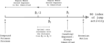
Figure 1: Two BG component model: regions where the components are identified versus not identified, and optimal rate of convergence.

The main results of the paper are summarized in Figure 1 for the two-component situation. We already noted that $\beta_{2}$ can be identified only if it is bigger than $\beta_{1}/2;$ we will also see that the rate at which $\beta_{2}$ can be estimated increases as $\beta_{2}$ gets closer to $\beta_{1}$, and conversely decreases as $\beta_{2}$ gets closer to $\beta_{1}/2$, in the limit dropping to $0$ as $\beta_{2}$ approaches $\beta_{1}/2$, consistently with the loss of identification that occurs at that point. Beyond the two-component model, we will provide general identifiability conditions and rates of convergence for the leading and higher order BG indices.

The paper is organized as follows. We first define the successive BG indices in Section 2. In Section 3, we study the identifiability of the parameters appearing in the expansion, from a theoretical viewpoint and in the special case of Lévy processes. Then we introduce consistent estimators for those parameters which we have found to be identifiable in the Lévy case, hence proving de facto their identifiability. This is done according to a two-step procedure, with preliminary estimators given in Section 4, and final estimators with much faster rates in Section 5. Unfortunately, although rates are given, we were not able to show a central limit theorem for these estimators, although such theorems ought to be available and would be crucial for obtaining confidence bounds.

In principle, those estimators could be used on real data, but the rates of convergence for the higher order indices are, by necessity, quite slow. We show in Section 6 that the slow nature of these rates of convergence is an inherent feature of the problem that cannot be improved upon. This is perhaps not too surprising since the range of values of the higher order indices that are identified is limited, and hence one would expect the rate of convergence to deteriorate all the way to zero as one approaches the region where identification disappears. We provide in Section 7 a simulation study for a model featuring a stochastic volatility plus two stable processes with different indices, the aim being to identify these two indices, especially the higher order one. A realistic application to high-frequency financial data, is out of the question for the typical sample sizes that are currently available, but may be useful in the future or in different fields of applications where semimartingales are used and where data are available in vast quantities, such as the study of Internet traffic or turbulence data in meteorology. The results do also present theoretical interest, especially as they set up bounds on what is asymptotically identifiable in the jump measure of a semimartingale, and consequently what is not.

2 The successive Blumenthal–Getoor indices

Throughout the paper, $X$ is an Itô semimartingale with characteristics given by (1), on a filtered probability space $(\Omega,\mathcal{F},(\mathcal{F}_{t})_{t\geq 0},\mathbb{P})$. The time horizon for the observations is $T>0$, so the behavior of $X$ after time $T$ does not matter for us below.

Our first aim is to give a precise meaning to an hypothesis like (4). Instead of requiring an expansion like this for all times $t$, we rather use the “integrated version” which uses the following family of (adapted, continuous and increasing) processes:

$$u>0\quad\Rightarrow\quad\overline{A}(u)_{t}=\int_{0}^{t}F_{s}([-u,u]^{c})\,ds.$$ (5)

The basic assumption is as follows:

Assumption 1.

There are a nonrandom integer $j$, a strictly decreasing sequence $(\beta_{i})_{1\leq i\leq j+1}$ of numbers in $[0,2)$ and a sequence $(A^{i})_{1\leq i\leq j+1}$ of processes such that

$$t\in[0,T],\qquad 0<u\leq 1\quad\Rightarrow\quad\Biggl{|}\overline{A}(u)_{t}-\sum_{i=1}^{j}\frac{A_{t}^{i}}{u^{\beta_{i}}}\Biggr{|}\leq\frac{A_{t}^{j+1}}{u^{\beta_{j+1}}}.$$ (6)

Moreover, we have $A^{i}_{T}>0$ for $i=1,\ldots,j$.

If this assumption is satisfied with some $j\geq 2$, it is also satisfied with any smaller integer. The processes $A^{i}$ and $A^{\prime}$ are nondecreasing nonnegative, and they can always be chosen to be predictable.

Clearly, $\beta=\beta_{1}$ is the BG index, as introduced before, and the following definition comes naturally in:

Definition 1.

Under Assumption 1, the numbers $\beta_{1},\beta_{2},\ldots,\beta_{j}$ are called the successive BG indices of the process $X$ over the time interval $[0,T]$, and the variables $A^{i}_{T}$ are called the associated integrated intensities.

Example 1.

Let $Y^{1},\ldots,Y^{j}$ be independent stable processes with indices $\beta_{1}>\cdots>\beta_{j}$. Then $X=Y^{1}+\cdots+Y^{j}$ satisfies (6) with $A^{j+1}=0$ and the successive indices and integrated intensities are $\beta_{i}$ and $Ta_{i}$, where $a_{i}=\lim_{u\to 0}u^{\beta_{i}}F^{i}([-u,u]^{c})$, and $F^{i}$ is the Lévy measure of $Y^{i}$.

If the $Y^{i}$’s are tempered stable processes [see Rosiński (2007)] the same is true, provided $\beta_{j}>\beta_{1}-1$.

Example 2.

A semimartingale consisting of a continuous component and a jump part driven by a sum of such processes also satisfies (6). Let $X_{t}=X_{0}+Z_{t}+\sum_{i=1}^{j}\int_{0}^{t}H_{s}^{i}\,dY_{s}^{i}$, with $Z$ a continuous Itô semimartingale and $Y^{i}$ as in the previous example and $H^{i}$ locally bounded predictable processes with $\int_{0}^{T}|H^{i}_{s}|^{\beta_{i}}\,ds>0$. The successive BG indices are again the $\beta_{i}$’s, with the associated integrated intensities

$$A_{T}^{i}=a_{i}\int_{0}^{T}|H_{s}^{i}|^{\beta_{i}}\,ds.\vspace*{-2pt}$$

Remark 1.

We have taken a finite family of possible indices $\beta_{i}$. Nothing prevents us from taking an infinite sequence: we simply have to assume that Assumption 1 holds for all $j$, with additionally $\lim_{i\to\infty}\beta_{i}=0$. However, in view of the restriction imposed on the BG indices by our main theorems below about identifiability, this more general situation has no statistical interest.

Remark 2.

Assumption 1 imposes a certain structure on the behavior of the jump measure of the process near $0$. It is important to note that it does not restrict in any way the behavior of the jump measure away from $0$. Although most models used in practice and with infinite activity jumps satisfy this assumption, the Gamma process does not: although it (barely) exhibits infinite activity, its BG index is $0$, and $\overline{A}(u)_{t}$ is of order $\log(1/u)$.

In Assumption 1, expansion (6) is central, but one may wonder about the additional requirement $A^{i}_{T}>0$. So, we end this section with some comments and extensions, which may look complicated and are not necessary for the rest of the paper, but which we think are useful and somewhat enlightening.

Extension 1.

In Assumption 1 positive and negative jumps are treated in the same way. In practice, it might be useful for modeling purposes to establish the behavior of positive and negative jumps separately. Toward this end, one can replace (5) by

$$\overline{A}(u)_{t}^{(+)}=\int_{0}^{t}F_{s}((u,\infty))\,ds,\qquad\overline{A}(u)_{t}^{(+)}=\int_{0}^{t}F_{s}((-\infty,-u))\,ds.$$

Then, if one is interested in positive jumps only, say, one replaces (6) by a similar expansion for $\overline{A}(u)_{t}^{(+)}$: all the content of the paper still holds, mutatis mutandis, under this modified assumption, for positive jumps. The same is true of negative jumps, and the “positive” and “negative” successive BG indices can of course be different.

Extension 2.

Now we come to the requirement $A^{i}_{T}>0$, which in Assumption 1 is supposed to hold for all (or, almost all) $\omega$. This is of course unlikely to hold for the terminal time $T$, unless it holds for all $t>0$, and even unless the processes $A^{i}$ are strictly increasing. In Example 2, this amounts to suppose that none of processes $H^{i}$ vanishes. However, it might be relevant in practice to allow for each $H^{i}$ to vanish on some (possibly random) time intervals: we then can have different components of the model turned on and off at different times.

Thus, let us examine what happens if we relax the requirements $A^{i}_{T}>0$. For any particular outcome $\omega$, the (first) BG index of the process $X$ is $\beta_{i}$, where $i$ is the smallest integer such that $A^{i}_{T}>0$, and if all of them vanish one only knows that the BG index is not bigger than $\beta_{j+1}$. The same applies to further indices. In other words, one can define a partition of $\Omega$ indexed by all subsets $D$ of $\{1,\ldots,j\}$ as follows:

$$\Omega_{T}(D)=\biggl{(}\bigcap_{i\in D}\{A_{T}^{i}>0\}\biggr{)}\cap\biggl{(}\bigcap_{i\in\{1,\ldots,j\}\setminus D}\{A_{T}^{i}=0\}\biggr{)}.$$ (7)

Then, for any $\omega$, the successive BG indices of $X$ over $[0,T]$ and the associated intensities are the numbers $\beta^{\prime}_{1}(\omega),\ldots,\beta^{\prime}_{J}(\omega)$ and $\Gamma_{i}(\omega)$, defined as

$$J(\omega) = m,\qquad\beta^{\prime}_{i}(\omega)=\beta_{l_{i}},$$

$$\Gamma_{i}(\omega) = A_{t}^{l_{i}}(\omega)\qquad\mbox{if }\omega\in\Omega_{t}(\{l_{1},\ldots,l_{m}\}).$$

On the set $\Omega_{T}(\varnothing)$, which is not necessarily empty, we have $J=0$ and no $\beta^{\prime}_{i}$’s.

All results of this paper are true if we relax $A^{i}_{T}>0$ in Assumption 1, provided we replace $j$ by $J$ and the $\beta_{i}$’s by the $\beta^{\prime}_{i}$’s, in restriction to the set $\Omega_{T}(D)$: this is indeed very easy, because on this set the process $X$ coincides at all times $t\in[0,T]$ with a process $X^{\prime}$ with satisfies Assumption 1 as stated above, with $(j,\beta_{1},\ldots,\beta_{j},\beta_{j+1})$ substituted with $(m,\beta_{l_{1}},\ldots,\beta_{j_{m}},\beta_{j+1})$, when $D=\{l_{1},\ldots,l_{m}\}$.

3 Identifiability in the Lévy case

Loosely speaking, in an asymptotic statistical framework, identifiability of a parameter means the existence of a sequence of estimators which is (weakly) consistent. Identifiability can be “proved” by exhibiting such a sequence. It can be “disproved” by theoretical arguments, such as the fact that if the parameter is identifiable in our high-frequency observations setting, then, were the path $t\mapsto X_{t}$ fully observed on $[0,T]$, it would enjoy “nonasymptotic” identifiability in the sense that its value is almost surely known. For example, in the simple model $X_{t}=bt+W_{t}$ the parameter $b$ does not enjoy this nonasymptotic property because the laws of the process $X$ (restricted to $[0,T]$) are all equivalent when $b$ varies, and thus $b$ is even less identifiable in the asymptotic setting.

Disproving identifiability is usually a hard task, especially in a nonparametric setting. However, if a parameter is not identifiable for a certain class of models, it is of course not identifiable for any wider class.

These arguments lead us to consider the very special situation of a Lévy processes $X$, with Lévy–Khintchine characteristics $(b,c,F)$ [see (2)] when the path $t\mapsto X_{t}$ is fully observed on $[0,T]$. In this section we are interested in nonasymptotic identifiability of those characteristics, or functions of them. Note that, were $T$ infinite, the triple $(b,c,F)$ would be identifiable because, for example, one would know the values of all the i.i.d. increments $X_{n+1}-X_{n}$, giving us almost surely the law of $X_{1}$, which in turn determines the triple $(b,c,F)$.

This is no longer the case when, as in this paper, the time interval $[0,T]$ is finite. In this case, we give a formal definition of identifiability. We use $Q_{b,c,F}$ to denote the law of the process $X$, restricted to the interval $[0,T]$ ($T$ is kept fixed all throughout). So $Q_{b,c,F}$ is a probability measure on the Skorokhod space $\mathbb{D}=\mathbb{D}(|0,T],\mathbb{R})$. We also let $\mathcal{T}$ be some given subset of all possible triples $(b,c,F)$.

Definition 2.

A function $H$ is identifiable on the class $\mathcal{T}$ if, for any two $(b,c,F)$ and $(b^{\prime},c^{\prime},F^{\prime})$ in $\mathcal{T}$ such that $H(b^{\prime},c^{\prime},F^{\prime})\neq H(b,c,F)$, we have $Q_{b,c,F}\perp Q_{b^{\prime},c^{\prime},F^{\prime}}$ (i.e., the two measures $Q_{b,c,F}$ and $Q_{b^{\prime},c^{\prime},F^{\prime}}$ are mutually singular).

The rationale behind this definition is as follows: if $H$ is identifiable and $(b,c,F)\in\mathcal{T}$, and $X$ is drawn according to the law $Q_{b,c,F}$, then we can discard with probability $1$ any fixed $(b^{\prime},c^{\prime},F^{\prime})\in\mathcal{T}$ such that $H(b^{\prime},c^{\prime},F^{\prime})\neq H(b,c,F)$. Unfortunately, this does not mean that we can (almost surely) reject all $(b^{\prime},c^{\prime},F^{\prime})$ with $H(b^{\prime},c^{\prime},F^{\prime})\neq H(b,c,F)$ simultaneously: this stronger property is (almost) never satisfied.

There exists a criterion for mutual singularity of $Q_{b,c,F}$ and $Q_{b^{\prime},c^{\prime},F^{\prime}}$; see Remark IV.4.40 of Jacod and Shiryaev (2003). We have a Lebesgue decomposition $F^{\prime}=f\bullet F+F^{\prime}{}^{\perp}$ of $F^{\prime}$ with respect to $F$, with $f$ a nonnegative Borel function and $F^{\prime}{}^{\perp}$ a measure supported by an $F$-null set. Then $Q_{b^{\prime},c^{\prime},F^{\prime}}\perp Q_{b,c,F}$ if and only if at least one of the following five properties is violated:

$$\cases{\displaystyle F^{\prime}{}^{\perp}(\mathbb{R})<\infty,\vspace*{2pt}\cr\displaystyle\alpha(F,F^{\prime})=\int\bigl{(}|f(x)-1|^{2}\wedge|f(x)-1|\bigr{)}F(dx)<\infty,\vspace*{2pt}\cr\displaystyle\alpha^{\prime}(F,F^{\prime})=\int_{\{|x|\leq 1\}}|x||f(x)-1|F(dx)<\infty,\vspace*{2pt}\cr\displaystyle c=0\quad\Rightarrow\quad b^{\prime}=b-\int_{\{|x|\leq 1\}}x\bigl{(}f(x)-1\bigr{)}F(dx),\cr c^{\prime}=c.}$$ (9)

It clearly follows that the function $H(b,c,F)=c$ is identifiable on any class $\mathcal{T}$ (a well-known fact). The function $H(b,c,F)=b$ is not identifiable in general; however, on the class of all $(b,c,F)$ having $c=0$ and $\int_{\{|x|\leq 1\}}|x|F(dx)<\infty$ the function $H(b,c,F)=\widehat{b}=b-\int_{\{|x|\leq 1\}}xF(dx)$ (which is the “real” drift, in the sense that $X_{t}=\widehat{b}t+\sum_{s\leq t}\Delta X_{s}$) is identifiable.

In the sequel we are not interested in $b$ or $c$, but in $F$ only. That is, we are looking at functions $H=H(F)$. This leads us to consider classes of the form

$$\mathcal{T}=\mathbb{R}\times\mathbb{R}_{+}\times\mathcal{T}_{3}\qquad\mbox{where }\mathcal{T}_{3}\mbox{ is a set of L\'{e}vy measures.}$$ (10)

In words, we want no restriction on the parameters $b$ and $c$. Of course $\mathcal{T}_{3}$ should not be a singleton, and $H(F)$ should not be constant on $\mathcal{T}_{3}$, otherwise the identifiability problem is empty.

The following example is clear:

Example 3.

If $\mathcal{T}_{3}$ is a set of measures which coincide with some given $F$ on a neighborhood of $0$, then by (9) no nontrivial $H(F)$ is identifiable on $\mathcal{T}$.

This implies that, in the best-case scenario, a function $H(F)$ can be identifiable only if it depends on the “behavior of the measure $F$ around $0$.” Giving a necessary and sufficient condition for identifiability of such a function, other than saying that one of the properties in (9) fails when $H(F)\neq H(F^{\prime})$, seems out of reach. However, this is possible for some specific, but relatively large, classes of sets $\mathcal{T}_{3}$, with a priori relatively surprising results. Below we introduce such a class, in order to illustrate the nature of the available results.

Definition 3 ((The class $\mathcal{T}_{3}^{(1)}$ of Lévy measures)).

We say that a Lévy measure $F$ belongs to this class if we have

$$\quad\cases{\displaystyle F(dx)=\widetilde{F}(dx)+\sum_{i=1}^{\infty}\frac{a_{i}\beta_{i}}{|x|^{1+\beta_{i}}}1_{[-\eta,\eta]}(x)\,dx,\qquad\mbox{where $\eta>0$ and}\vspace*{2pt}\cr\displaystyle\qquad\mbox{\hphantom{ii}(i)\quad}0\leq\beta_{i+1}\leq\beta_{i}<2,\qquad\beta_{i}>0\quad\Rightarrow\quad\beta_{i}>\beta_{i+1},\vspace*{2pt}\cr\displaystyle\qquad\mbox{\hphantom{(iii)}\quad}\lim_{i\rightarrow\infty}\beta_{i}=0,\vspace*{2pt}\cr\displaystyle\qquad\mbox{\hphantom{i}(ii)\quad}a_{i}>0\quad\Leftrightarrow\quad\beta_{i}>0,\vspace*{2pt}\cr\displaystyle\qquad\mbox{(iii)\quad}0<\sum_{i=1}^{\infty}a_{i}<\infty,\vspace*{2pt}\cr\displaystyle\qquad\mbox{\hskip 1.0pt(iv)\quad}\widetilde{F}\mbox{ is a finite measure supported by }[-\eta,,\eta]^{c}.}$$ (11)

Parts (i) and (ii) together ensure the uniqueness of the numbers $(a_{i},\beta_{i})$ in the representation of $F$, whereas if this representation holds for some $\eta>0$, it also holds for all $\eta^{\prime}\in(0,\eta)$, with the same $(a_{i},\beta_{i})$. Part (iii) ensures that the infinite sum in the representation converges, without being zero (so equivalently, $a_{1}>0$, or $\beta_{1}>0$).

The class $\mathcal{T}_{3}^{(1)}$ contains all sums of symmetric stable Lévy measures. On the other hand, it is contained in the class of all Lévy measures $F$ of a Lévy process satisfying Assumption 1: the latter is the class $\mathcal{T}_{3}^{(2)}$ of all $F$ such that

$$u\leq 1\quad\Rightarrow\quad\Biggl{|}F([-u,u]^{c})-\sum_{i=1}^{j}\frac{a_{i}}{u^{\beta_{i}}}\Biggr{|}\leq\frac{a^{\prime}}{u^{\beta_{j+1}}}$$ (12)

for $2>\beta_{1}>\cdots>\beta_{j+1}\geq 0$ and $a_{i}>0$ for $i=1,\ldots,j$ and $a^{\prime}\geq 0$, and those conditions are implied by (11), for any $j\leq\sup(i\dvtx\beta_{i}>0)$, with the same $\beta_{i}$ and $a_{i}$.

Considering $a_{i}$ and $\beta_{i}$ as functions on $\mathcal{T}_{3}^{(1)}$, the identifiability result goes as follows:

Theorem 1

In the previous setting, the following holds:

The functions $\beta_{1}$ and $a_{1}$ are identifiable on the set $\mathcal{T}^{(1)}_{3}$.

For any given $i\geq 2$, the functions $\beta_{i}$ and $a_{i}$ are identifiable on the subset $\mathcal{T}^{(1)}_{3}(i)=\{F\in\mathcal{T}^{(1)}_{3}\dvtx\beta_{i}(F)\geq\beta_{1}(F)/2\}$ of $\mathcal{T}^{(1)}_{3}$, and they are not on the complement $\mathcal{T}^{(1)}_{3}\setminus\mathcal{T}^{(1)}_{3}(i)$.

Remark 3.

As mentioned in the “first extension” described in the previous section, a similar statement is true if we replace the first line of (11) by

$$F(dx)=\widetilde{F}(dx)+\sum_{j=1}^{\infty}\biggl{(}\frac{a_{i}^{(+)}\beta_{i}^{(+)}}{|x|^{1+\beta_{i}}}1_{(0,\eta]}(x)+\frac{a_{i}^{(-)}\beta_{i}^{(-)}}{|x|^{1+\beta_{i}}}1_{(-\eta,0)}(x)\biggr{)}\,dx$$

with both families $(\beta_{i}^{(\pm)},a_{i}^{(\pm)})$ satisfying (i)–(iii). Then the theorem above holds for both these families, with exactly the same proof.

Remark 4.

As said before, any Lévy process $X$ whose Lévy measure $F$ is in $\mathcal{T}_{3}^{(1)}$ satisfies Assumption 1, but the converse is far from being true, so, even for Lévy processes, the identifiability question is not completely solved under Assumption 1. More precisely, as the estimation results will show below, (12) implies the “positive” identifiability results [(i) and the first part of (ii) of Theorem 1] for Lévy processes, but not the “negative” results [second part of (ii)].

For example, consider the class $\mathcal{T}_{3}^{(3)}$ of all measure of the form

$$F(dx)=\frac{a_{1}\beta_{1}}{x^{1+\beta_{1}}}1_{(0,1]}(x)\,dx+G(dx)\qquad\mbox{with }G=a_{2}\sum_{n\geq 1}\varepsilon_{1/n^{1/\beta_{2}}}(dx)$$

and $0<\beta_{2}<\beta_{1}<2$ and $a_{1},a_{2}>0$. Any such $F$ satisfies (34), but not (11). On $\mathcal{T}_{3}^{(3)}$, all four parameters $\beta_{1},\beta_{2},a_{1},a_{2}$ are identifiable without the restriction $\beta_{2}\geq\beta_{1}/2$. This is of course due to the fact that the measure $G$ is singular, and any two measures $G$ and $G^{\prime}$ of the same type with $(\beta_{2},a_{2})\neq(\beta_{2}^{\prime},a_{2}^{\prime})$ have a Lebesgue decomposition $G^{\prime}=g\bullet G+G^{\prime\perp}$ with $G^{\prime\perp}(\mathbb{R})=\infty$ when $\beta_{2}\neq\beta_{2}^{\prime}$ and $\alpha(G,G^{\prime})=\infty$ when $\beta_{2}=\beta_{2}^{\prime}$ and $a_{2}\neq a_{2}^{\prime}$.

We emphasize again that this example is quite singular, and verify here the fairly general principle that the less regular a statistical problem is, the easier it is to solve in the sense that more parameters can be estimated, and often with faster rates.

Remark 5.

The class $\mathcal{T}_{3}^{(2)}$ may be bigger than $\mathcal{T}_{3}^{(1)}$, but it is very far from containing all possible Lévy measures. Indeed, any decreasing right-continuous function $f$ on $(0,\infty)$ with $f(x)\to 0$ as $x\to\infty$ and $f(x)\leq K/x^{\alpha}$ for $x\in(0,1]$, for some constants $K>0$ and $\alpha\in(0,2)$, is the symmetrical tail $f(x)=F([-x,x]^{c})$ of a Lévy measure, although of course it does not need to be equivalent to $a/x^{\beta}$ as $x\to 0$ for some $\beta\in(0,2)$ and $a>0$: so (6) may fail even with $j=1$.

4 Discretely observed semimartingales: Preliminary estimators

Now we turn to the more general case of semimartingales. The process $X$ is observed at the times $i\Delta_{n}$ for $i=0,1,\ldots,[T/\Delta_{n}]$ (where $[x]$ denotes the integer part of the real $x$). We thus observe the increments

$$\Delta_{i}^{n}X=X_{i\Delta_{n}}-X_{(i-1)\Delta_{n}}.$$ (13)

The BG indices describes some properties of jumps, which are not observed. However, when an increment $\Delta_{i}^{n}X$ is relatively large, say bigger than $u_{n}$ with $u_{n}\gg\sqrt{\Delta_{n}}$, it is likely to be due to jumps because the drift plus the continuous martingale part have increments of order of magnitude $\sqrt{\Delta_{n}}$. Moreover it turns out that it is usually due to a single “large” jump of size bigger than $u_{n}$, although of course the observed value $\Delta^{n}_{i}X$ is not exactly the jump size. So one may expect the number of jumps with size bigger than $u_{n}=u$, over the time interval $[0,t]$, to be the following number, or be relatively close to it:

$$U(u,\Delta_{n})_{t}=\sum_{i=1}^{[t/\Delta_{n}]}1_{\{\Delta_{i}^{n}X>u\}}.$$ (14)

In order for the previous statement to actually be true, we need some additional assumptions, though. Those are given in the following:

Assumption 2.

The process $X$ is an Itô semimartingale, and:

[(a)]

The processes $b_{t}$, $c_{t}$ are locally bounded.

We have Assumption 1 with $A_{t}^{i}=\int_{0}^{t}a_{s}^{i}\,ds$ for $i=1,\ldots,j+1$, where the processes $a^{i}$ are locally bounded.

We have $\beta_{j}>\beta_{1}/2$.

Assumption 2(c) above may look strange, or too strong. However, in view of the identifiability results of the previous section, we cannot estimate consistently $\beta_{i}$ if it is strictly smaller than $\beta_{1}/2$, and as a matter of fact, the estimators described below are consistent only if $\beta_{i}>\beta_{1}/2$. Hence, since Assumption 1 for $j$ implies the same for all $j^{\prime}<j$, (c) above is really not a restriction, but amounts to replacing $j$ in this assumption by $j\wedge\sup\{i\dvtx\beta_{i}>\beta_{1}/2\}$.

Apart from (c), this assumption is satisfied in Examples 1 and 2, and also by any Lévy process satisfying Assumption 1.

The estimation procedure is a two-step procedure, and in this section we describe the first—preliminary—estimators. These estimators will be consistent, but with very slow rates of convergence. This is why, in the next subsection, we will derive final estimators which exhibit much faster (although still slow) rates.

Those preliminary estimators require the knowledge of a number $\varepsilon>0$ which satisfies

$$i=1,\ldots,j-1\quad\Rightarrow\quad\beta_{i}-\beta_{i+1}\geq\varepsilon.$$ (15)

Such an $\varepsilon$ always exists, but here we suppose that it is known, somewhat in contradiction with the fact that the $\beta_{i}$ are unknown. It it is obviously quite difficult to estimate properly two contiguous indices $\beta_{i}$ and $\beta_{i+1}$ when they are very close to to one another. So from a statistical viewpoint, the assumption $\beta_{i}-\beta_{i+1}>\varepsilon$ for some fixed $\varepsilon>0$ is natural. Moreover, since we do not know a priori which $\omega$ is observed, this amounts to supposing that all possible values of the BG indices in the model satisfy this restriction. For models used in practice, this is not really a restriction since these models rely on at most a small number of indices that are separated from one another.

The key ingredient for constructing the estimators is the counting process defined in (14), evaluated at the terminal time $T$ and for suitable values of $u$. In particular, we choose a sequence $u_{n}$ satisfying

$$u_{n}\rightarrow 0,\qquad\Delta_{n}^{\rho}\leq Ku_{n}\hskip 40.0pt$$ (17)

$$\eqntext{\mbox{with }\displaystyle\rho<\frac{1}{2+\beta_{1}}\wedge\frac{2}{\beta_{1}(3+\beta_{1})}\wedge\frac{4}{\beta_{1}(5+3\beta_{1})}.}$$

Of course $\rho>0$ above (otherwise $u_{n}\rightarrow 0$ would fail). The infimum of the upper bound for $\rho$ over all $\beta_{1}<2$ is $2/11$. Therefore, since we do not a priori know the values of $\beta_{1}$, whereas as we will see the rates improve when the sequence $u_{n}$ becomes smaller (termwise), it is thus advisable to take $\rho=2/11$ above.

The first-step estimation is done by induction on $i$. We choose $\gamma>1$, and the estimators for $\beta_{1}$ and $A_{T}^{1}$ are

$$\qquad\widetilde{\beta}_{1}^{n} = \cases{\displaystyle\frac{\log(U(u_{n},\Delta_{n})_{T}/U(\gamma u_{n},\Delta_{n})_{T})}{\log\gamma},&\quad if $U(\gamma u_{n},\Delta_{n})_{T}>0$,\vspace*{2pt}\cr-1,&\quad otherwise,}$$

$$\widetilde{\Gamma}_{i}^{n} = (u_{n})^{\widetilde{\beta}_{1}^{n}}U(u_{n},\Delta_{n})_{T}.$$

For constructing the subsequent estimators, and with $\varepsilon$ in (15), we set

$$u_{n,i}=u_{n}^{(\varepsilon/2)^{i-1}}$$ (19)

(so $u_{n,1}=u_{n}$). We denote by $I(k,l)$ the set of all subsets of $\{1,\ldots,k\}$ having $l$ elements. Assuming that we know $\widehat{\beta}_{i}^{n}$ and $\widehat{\Gamma}_{i}^{n}$ for $i=1,\ldots,k-1$, for some $k\in\{2,\ldots,j\}$, we set

$$x \geq 1\quad\Rightarrow\quad U^{n}(k,x)=\sum_{l=0}^{k-1}(-1)^{l}U(x\gamma^{l}u_{n,k},\Delta_{n})_{T}\sum_{J\in I(k-1,l)}\gamma^{\sum_{i\in J}\widetilde{\beta}_{i}^{n}},$$

$$\widetilde{\beta}_{k}^{n} = \cases{\displaystyle\frac{\log(U^{n}(k,1)/U^{n}(k,\gamma))}{\log(\gamma)},&\quad if $U^{n}(k,1)>0,U^{n}(k,\gamma)>0$,\vspace*{2pt}\cr-1,&\quad otherwise,}$$ (20)

$$\widetilde{\Gamma}_{k}^{n} = u_{n,k}^{\widetilde{\beta}_{k}^{n}}\Biggl{(}U(u_{n,k},\Delta_{n})_{T}-\sum_{l=1}^{k-1}\widetilde{\Gamma}_{l}^{n}u_{n,k}^{-\widetilde{\beta}_{l}^{n}}\Biggr{)}.$$

Finally, in order to state the result, we need a further notation, for $i=1,\ldots,j-1$ (so when $j=1$ the following is empty):

$$H_{i}=\frac{A_{T}^{i+1}}{A_{T}^{i}\log\gamma}\frac{\prod_{l=1}^{i}(\gamma^{\beta_{l}-\beta_{i+1}}-1)}{\prod_{l=1}^{i-1}(\gamma^{\beta_{l}-\beta_{i}}-1)}.$$ (21)

Theorem 2

Under Assumption 2 and (15), for all $i=1,\ldots,j-1$ such that $\beta_{i+1}>\beta_{1}/2$, we have

$$\frac{\widetilde{\beta}_{i}^{n}-\beta_{i}}{u_{n,i}^{\beta_{i}-\beta_{i+1}}}\stackrel{{\scriptstyle\mathbb{P}}}{{\longrightarrow}}-H_{i},\qquad\frac{\widetilde{\Gamma}_{i}^{n}-A_{T}^{i}}{u_{n,i}^{\beta_{i}-\beta_{i+1}}\log(1/u_{n,i})}\stackrel{{\scriptstyle\mathbb{P}}}{{\longrightarrow}}\Gamma_{i}H_{i}.$$ (22)

Moreover if $\eta=\beta_{j}-\beta_{j+1}\vee\frac{\beta_{1}}{2}>0$, the following variables are bounded in probability:

$$\frac{\widetilde{\beta}_{j}^{n}-\beta_{i}}{u_{n,j}^{\eta}},\qquad\frac{\widetilde{\Gamma}_{j}^{n}-A_{T}^{j}}{u_{n,j}^{\eta}\log(1/u_{n,j})}.$$ (23)

The estimator $\widetilde{\beta}_{1}^{n}$ is exactly the estimator proposed in Aït-Sahalia and Jacod (2009a) for the leading BG index $\beta_{1}$. So, not only does it satisfy (22) when $j\geq 2$ or the tightness of (23) when $j=1$, but it also enjoys a central limit theorem centered at $\beta_{1}$ and with rate $u_{n}^{\beta_{1}/2}$ as soon as $\beta_{2}<\beta_{1}/2$ (this property implies $j=1$ here). Moreover, in this case one could prove that $\widetilde{\Gamma}_{1}^{n}$ also satisfies a CLT with the rate $u_{n}^{\beta_{1}/2}\log(1/u_{n})$, although we will not prove it, since the emphasis here is on the case of several BG indices.

Some remarks are in order here:

Remark 6.

It is possible for the estimator $\widetilde{\Gamma}^{n}_{i}$ to be negative, in which case we may replace it by $0$, or by any other positive number. It may also happen that the sequence $\widetilde{\beta}^{n}_{i}$ is not decreasing, and we can then reorder the whole family as to obtain a decreasing family (we relabel the estimators of $A_{T}^{i}$ accordingly, of course). All these modifications are asymptotically immaterial.

Remark 7.

As mentioned in the Extension 2 at the end of Section 2, we can relax $A^{i}_{T}>0$ in Assumption 1. Then the above theorem is still valid, in restriction to the set $\Omega_{T}(\{l_{1},\ldots,l_{m}\})$ of (7), as soon as $\beta_{l_{m}}>\beta_{l_{1}}/2$.

Remark 8.

Suppose that $j\geq 2$. The limits in (22) are pure bias, hence precluding the existence of a proper central limit theorem. Note that $H_{i}>0$ if $i<j$, so the bias for $\widehat{\beta}_{i}^{n}$ and for $\widehat{\Gamma}_{i}^{n}$ are always negative and positive, respectively.

Note also that the rate of convergence for estimating $\beta_{i}$ when $i\leq j-1$, say, is $u^{\beta_{i}-\beta_{i+1}}_{n,i}$, that is $u_{n}^{(\beta_{i}-\beta_{i+1})(\varepsilon/2)^{i-1}}$. This is exceedingly small, indeed. For example, suppose that we have three indices $\beta_{1}>\beta_{2}>\beta_{3}>\frac{\beta_{1}}{2}$. Then (15) implies necessarily $\varepsilon<\frac{\beta_{1}}{2}$, so the best possible rate for $i=2$ would be less than, but close to, $u_{n}^{(\beta_{2}-\beta_{3})\beta_{1}/4}$, upon taking $\varepsilon$ close to $\frac{\beta_{1}}{2}$, which is of course impossible because we do not know $\beta_{1}$ to start with.

In the previous example, if we suspect that $\beta_{1}$ is bigger than $1$, say, it becomes (perhaps) not totally unreasonable to choose $\varepsilon=0.1$; the rates for $i=2$ and $i=3$ thus become $u_{n}^{(\beta_{2}-\beta_{3})/10}$ and $u_{n}^{(\beta_{3}-\beta_{1}/2)/100}$. This is of course on top of the fact that, because of (17), $u_{n}$ is of order of magnitude $\Delta_{n}^{2/11}$, by a conservative choice of $\rho$.

Practical considerations. Letting aside the slow convergence rates, the previous result suffers from two main drawbacks:

(1) It requires to know the number of indices to be estimated (this is implicit in Assumption 2).

(2) It requires to know a number $\varepsilon>0$ satisfying (15).

About the first problem above, in real world one does not know the number of indices. On the other hand, if Assumption 1 holds, it seems reasonable to suppose that it holds for all $j$, whereas the estimation is made for those $\beta_{i}$ which are bigger than $\beta_{1}/2$ only. In connection with this, we assume $\beta_{i}-\beta_{i+1}\geq\varepsilon$ for all $i\leq j:=\sup(k\dvtx\beta_{k}>\beta_{1}/2)$, plus the property $\beta_{j}>\beta_{1}/2+\varepsilon$. Then the aim becomes to estimate $\beta_{i}$ and $A^{i}_{T}$ for all $i\leq j$, with $j$ unknown.

Since the estimation procedure is done by induction on the successive indices, one can start the induction as described above, and stop it at the first $i$ such that $\widetilde{\beta}_{i}\leq\varepsilon+\widetilde{\beta}_{1}/2$. Asymptotically, this procedure will deliver the “correct” answer (the proof of this fact, not given below, is a simple extension of the proof of the second claim of the theorem). In practice, however, the solution to this stopping problem is not quite clear, since in particular the estimated sequence $\widetilde{\beta}_{i}$ is not necessarily decreasing, although it is so asymptotically.

Problem 2 above is clearly more annoying. We have to admit that, in the setting presented here, we have no theoretical solution for solving it. A possible way out would be to make the estimation with several values of $\varepsilon$, going downward, until the estimated differences $\widetilde{\beta}_{i}-\widetilde{\beta}_{i-1}$ all become significantly bigger than the chosen $\varepsilon$, but no mathematical result so far is available in this direction. In addition, since rates are very slow, the probability that such a difference is bigger than $\varepsilon$ when the true values satisfy the same inequality may be not close to $1$ (for finite, but even large, samples).

Nonetheless, bad as it looks, this condition is probably relatively innocuous in practice: indeed, when two successive indices are very close to each other, they are obviously very difficult to tell apart. So the problem is practically meaningful only if the indices are a small number (as $2$, $3$ or perhaps $4$) and reasonably well separated. Hence taking $\varepsilon=0.1$ for instance, as in Remark 5, seems to be safe enough.

5 Discretely observed semimartingales: An improved method

The observation scheme is the same as in the previous section: $X$ is observed at the times $i\Delta_{n}$ smaller or equal to some fixed terminal time $T$.

As already mentioned, the previous estimators converge at a very slow rate, especially for higher order indices; see Remark 8. So, in order to implement the estimation with any kind of reasonable accuracy, it is absolutely necessary to come up with better estimators.

This is the aim of this section. Assuming Assumption 2, we also suppose that we can construct preliminary estimators, such as in the previous section. Exactly as there, we must know the number $j$ of BG indices that are to be estimated.

The method consists in minimizing, at each stage $n$, a suitably chosen contrast function $\Phi_{n}$. First we take an integer $L\geq 2j$ and numbers $1=v_{1}<v_{2}<\cdots<v_{L}$. We also choose positive weights $w_{k}$ (typically $w_{k}=1$, but any choice is indeed possible), and we pick truncation levels $u_{n}$ satisfying (17). We also let $D$ be the set of all $(x_{i},\gamma_{i})_{1\leq i\leq j}$ with $0\leq x_{j}\leq x_{j-1}\leq\cdots\leq x_{1}\leq 2$ and $\gamma_{i}\geq 0$. Then the contrast function is defined on $D$ by

$$\Phi_{n}(x_{1},\gamma_{1},\ldots,x_{j},\gamma_{j})=\sum_{l=1}^{L}w_{l}\Biggl{(}U(v_{l}u_{n},\Delta_{n})_{T}-\sum_{i=1}^{j}\frac{\gamma_{i}}{(v_{l}u_{n})^{x_{i}}}\Biggr{)}^{2},$$ (24)

where the sequence $u_{n}$ satisfies (17). Then the estimation goes as follows:

Step 1.

We construct preliminary estimators $\widetilde{\beta}^{n}_{i}$ (decreasing in $i$) and $\widetilde{\Gamma}^{n}_{i}$ (nonnegative) for $\beta_{i}$ and $A_{T}^{i}$ for $i=1,\ldots,j$, such that $(\widetilde{\beta}_{i}-\beta_{i})/u_{n}^{\eta}$ and $(\widetilde{\Gamma}_{i}-A_{T}^{i})/u_{n}^{\eta}$ go to $0$ in probability for some $\eta>0$. For example, we may choose those described in the previous section (see Remark 6): the consistency requirement is fulfilled for any $\eta<(\varepsilon/2)^{j}$.

Step 2.

We denote by $D_{n}$ the (compact and nonempty) random subset of $D$ defined by $D_{n}=\{(x_{i},\gamma_{i})\in D\dvtx|x_{i}-\widetilde{\beta}^{n}_{i}|\leq\alpha u_{n}^{\eta},|\gamma_{i}-\widetilde{\Gamma}^{n}_{i}|\leq\alpha u_{n}^{\eta},\forall i=1,\ldots,j\}$, for some arbitrary (fixed) $\alpha>0$. Then the final estimators $\overline{\beta}{}^{n}_{i}$ and $\overline{\Gamma}{}^{n}_{i}$ will be

$$(\overline{\beta}{}^{n}_{i},\overline{\Gamma}{}^{n}_{i})_{1\leq i\leq j}=\mathop{\arg\min}_{D_{n}}\Phi_{n}(x_{1},\gamma_{1},\ldots,x_{j},\gamma_{j}).$$ (25)

Theorem 3

Under Assumption 2, and for all choice of $v_{2},\ldots,v_{L}$ outside a $\lambda_{L-1}$-null set (depending on the $\beta_{i}$’s; $\lambda_{l}$ is the $l$-dimensional Lebesgue measure), the sequences

$$\frac{\overline{\beta}{}^{n}_{i}-\beta_{i}}{u_{n}^{\beta_{i}-\beta_{1}/2-\mu}},\qquad\frac{\overline{\Gamma}{}^{n}_{i}-\Gamma_{i}}{u_{n}^{\beta_{i}-\beta_{1}/2-\mu}}$$ (26)

are bounded in probability for all $i=1,\ldots,j$ and all $\mu>0$.

The rates obtained here are much faster than in Theorem 2: we replace $u_{n,i}^{\beta_{i}-\beta_{i+1}\vee(\beta_{1}/2)}$ by $u_{n}^{\beta_{i}-\beta_{1}/2}$, for two reasons: the exponent $\beta_{i}-\beta_{i+1}$ is bigger than $\beta_{i}-\beta_{i+1}\vee(\beta_{1}/2)$, unless $i=j$; more importantly, we replace the auxiliary truncation levels $u_{n,i}$ of (19) by the original sequence $u_{n}$, which is much smaller when $i\geq 2$, and only subject to (17). We will examine in the next section how far from optimality those rates are.

Remark 9.

As stated, and as seen from the proof, we only need $L=2j$, and choosing $L>2j$ does not improve the asymptotic properties. However, from a practical viewpoint, it is probably wise to take $L$ bigger than $2j$ in order to smooth out the contrast function somehow, especially for (relatively) small samples. A choice of the weights $w_{l}>0$ other than $w_{l}=1$, such as $w_{l}$ decreasing in $l$, may serve to put less emphasis on the large truncation values $u_{n}v_{l}$ for which less data are effectively used.

Remark 10.

The result does not hold (or at least we could not prove it) for all choices of the $v_{l}$’s, but only when $(v_{2},\ldots,v_{L})$ (recall $v_{1}=1$) does not belong to some Lebesgue-null set $G(\beta_{1},\ldots,\beta_{j})$. This seems a priori a serious restriction, because $(\beta_{1},\ldots,\beta_{j})$ is unknown. In practice, we choose a priori $(v_{2},\ldots,v_{L})$, so we may have bad luck, just as we may have bad luck for the outcome $\omega$ which is drawn$\ldots.$

We may also do the estimation for a number of different choices for the weights and/or values of $L\geq 2j$ and compare or average the results. This should contribute to weaken the numerical instability inherent to minimization problems such as (25). This numerical instability is similar to the one occurring in nonlinear regression problems.

We have to state, however, that these problems, just as those stated in the “practical considerations” of the previous section, are not fully addressed in this paper, and they are probably quite difficult to overcome. Our emphasis here is more on theoretical results, and on the possibility of performing the estimation with reasonable rates (see, however, Section 7 below, to see how the problem of finding a “good” $\varepsilon$ and doing preliminary estimation in our simulation study is skipped, without affecting the quality of the procedure in any noticeable way).

6 Optimality in a special case

6.1 Why the convergence rates are necessarily slow

Intuitively, the fact that we are right at the boundary between identifiability and lack thereof suggests that we should expect the rate, as we approach the loss of identifiability boundary, to deteriorate all the way to zero. In order to quantify precisely how slow the rates of convergence for the estimators of the second (and higher) index must be, even in ideal circumstances, we study a simple parametric model of the following form. Let $W$ be a Brownian motion and $Y^{1},Y^{2}$ be two independent standard symmetric stable processes, and set

$$X_{t}=bt+\sigma W_{t}+Y_{t}^{1}+Y_{t}^{2}.$$ (27)

Each $Y^{i}$ depends on two parameters, the index $\beta_{i}$ and a scale parameter $a_{i}$, the latter being characterized by the fact that the Lévy measure of $Y^{i}$ is

$$F^{j}(dx)=\frac{a_{j}\beta_{j}}{|x|^{1+\beta_{j}}}\,dx.$$ (28)

We have six parameters,

$$b\in\mathbb{R},\qquad c=\sigma^{2}>0,\qquad a_{1},a_{2}>0,\qquad 0<\beta_{2}<\beta_{1}<2,$$ (29)

among which $b$ is not identifiable, and $c,\beta_{1},a_{1}$ are identifiable, and $(\beta_{2},a_{2})$ are identifiable if and only if $\beta_{2}\geq\beta_{1}/2$. In what follows, we restrict our attention to the four parameters $\beta_{1},\beta_{2},a_{1},a_{2}$.

In order to find at which rate it is possible to estimate these four parameters, when $X$ is observed at the discrete times $(i\Delta_{n}\dvtx i=0,1,\ldots,[T/\Delta_{n}])$ and $\Delta_{n}\rightarrow 0$, we study the behavior of the Fisher information matrix. Due to the fact that $X$ is a Lévy process, the information matrix at stage $n$ is $[T/\Delta_{n}]$ times the information matrix obtained when we observe only the variable $X_{\Delta_{n}}$; since the variable $X_{\Delta}$ admits a density $x\mapsto p(_{\Delta}(x|c,\beta_{1},a_{1},\allowbreak\beta_{2},a_{2})$ which is $C^{\infty}$ in $x$, and also in $(c,\beta_{1},a_{1},\beta_{2},a_{2})$ on the domain defined by (29), it is no wonder that Fisher’s information $I_{\Delta}$ for a single observation $X_{\Delta}$ (recall $X_{0}=0$) exists, and we can study its behavior as $\Delta\rightarrow 0$.

Only the diagonal entries are important for the various rates of convergence, so we only need to focus on the following diagonal entries of this matrix:

$$I_{\Delta}^{\beta_{1}\beta_{1}},I_{\Delta}^{a_{1}a_{1}},I_{\Delta}^{\beta_{2}\beta_{2}},I_{\Delta}^{a_{2}a_{2}}.$$

The main result of this section follows, giving the asymptotic order of the relevant terms in Fisher’s information:

Theorem 4

We have the following equivalences, as $\Delta\rightarrow 0$:

$$I_{\Delta}^{\beta_{1}\beta_{1}} \sim \frac{a_{1}}{2(2-\beta_{1})^{\beta_{1}/2}c^{\beta_{1}/2}}\Delta^{1-\beta_{1}/2}(\log(1/\Delta))^{2-\beta_{1}/2},$$

$$I_{\Delta}^{a_{1}a_{1}} \sim \frac{2\beta_{1}c_{\beta_{1}}a_{1}^{\beta_{1}}}{(2-\beta_{1})^{\beta_{1}/2}\sigma^{\beta_{1}}a_{1}^{2}}\frac{\Delta^{1-\beta_{1}/2}}{(\log(1/\Delta))^{\beta_{1}/2}}$$

and also, provided $\beta_{2}>\beta_{1}/2$,

$$I_{\Delta}^{\beta_{2}\beta_{2}} \sim \frac{a_{2}^{2}\beta_{2}^{2}}{2a_{1}\beta_{1}(2\beta_{2}-\beta_{1})(2-\beta_{1})^{\beta_{2}-\beta_{1}/2}c^{\beta_{2}-\beta_{1}/2}}$$

$${}\times\Delta^{1-\beta_{2}+\beta_{1}/2}(\log(1/\Delta))^{2-\beta_{2}+\beta_{1}/2},$$

$$I_{\Delta}^{a_{2}a_{2}} \sim \frac{2\beta_{2}^{2}}{a_{1}\beta_{1}(2\beta_{2}-\beta_{1})(2-\beta_{1})^{\beta_{2}-\beta_{1}/2}c^{\beta_{2}-\beta_{1}/2}}\frac{\Delta^{1-\beta_{2}+\beta_{1}/2}}{(\log(1/\Delta))^{\beta_{2}-\beta_{1}/2}}.$$

Remark 11.

We are not concerned here with the identification and estimation of the volatility parameter $c$; the term $I_{\Delta}^{cc}$ in a simpler model has been studied in Aït-Sahalia and Jacod (2008), as well as $I_{\Delta}^{a_{1}a_{1}}$ when $a_{2}=0$ (i.e., when there is only one stable process on top of the Brownian motion). The asymptotic equivalent for the term $I_{\Delta}^{a_{1}a_{1}}$ of course reduces to (4.11) of that paper, with $\alpha=\beta_{1}$, $\beta=2$, $\theta=a_{1}$, up to a change of parametrization for $a_{1}$, since here we use the parametrization (28) which corresponds to the notation of Assumption 1, which is fulfilled here.

Coming back to the original problem, we deduce that it should be possible in principle to find estimators $\widehat{\beta}_{i}^{n}$ and $\widehat{a}_{i}^{n}$ having the following properties:

$$\frac{(\log(1/\Delta_{n}))^{1-\beta_{1}/4}}{\Delta_{n}^{\beta_{1}/4}}(\widehat{\beta}_{1}^{n}-\beta_{1}) \stackrel{{\scriptstyle\mathcal{L}}}{{\longrightarrow}} \mathcal{N}(0,1/T\mathcal{I}^{\beta_{1}\beta_{1}}),$$

$$\frac{1}{\Delta_{n}^{\beta_{1}/4}(\log(1/\Delta_{n}))^{\beta_{1}/4}}(\widehat{a}_{1}^{n}-a_{1}) \stackrel{{\scriptstyle\mathcal{L}}}{{\longrightarrow}} \mathcal{N}(0,1/T\mathcal{I}^{a_{1}a_{1}}),$$

$$\frac{(\log(1/\Delta_{n}))^{1-\beta_{2}/2+\beta_{1}/4}}{\Delta_{n}^{\beta_{2}/2-\beta_{1}/4}}(\widehat{\beta}_{2}^{n}-\beta_{2}) \stackrel{{\scriptstyle\mathcal{L}}}{{\longrightarrow}} \mathcal{N}(0,1/T\mathcal{I}^{\beta_{2}\beta_{2}}),$$

$$\frac{1}{\Delta_{n}^{\beta_{2}/2-\beta_{1}/4}(\log(1/\Delta_{n}))^{\beta_{2}/2-\beta_{1}/4}}(\widehat{a}_{2}^{n}-a_{2}) \stackrel{{\scriptstyle\mathcal{L}}}{{\longrightarrow}} \mathcal{N}(0,1/T\mathcal{I}^{a_{2}a_{2}}),$$

where $\mathcal{I}^{\beta_{1}\beta_{1}}$, $\mathcal{I}^{a_{1}a_{1}}$, $\mathcal{I}^{\beta_{2}\beta_{2}}$ and $\mathcal{I}^{a_{2}a_{2}}$ are the constants in front of the term involving $\Delta$ in the equivalences above, for $I_{\Delta}^{\beta_{1}\beta_{1}}$, $I_{\Delta}^{a_{1}a_{1}}$, $I_{\Delta}^{\beta_{2}\beta_{2}}$ and $I_{\Delta}^{a_{2}a_{2}}$, respectively. Conversely, by the Cramér–Rao lower bound, Theorem 4 also implies that it will be impossible to find consistent estimators with faster rates of convergence, or smaller asymptotic variance, that those exhibited in (6.1).

Note that these rates are consistent with the results of Theorem 1. The first two convergences above shows that it is always possible to estimate consistently $\beta_{1}$ and $a_{1}$, the third one implies consistency for $\beta_{2}$ only if $\beta_{2}\geq\beta_{1}/2$, and the last one implies consistency for $a_{2}$ only if $\beta_{2}>\beta_{1}/2$. The last statement seems contradictory with Theorem 1 when $\beta_{2}=\beta_{1}/2$, but of course it is possible to have a (somewhat irregular) statistical model for which consistency holds even though the Fisher information does not go to infinity.

6.2 Comparison of rates

Now, we can compare these optimal rates with the rates obtained in Theorem 3. Doing as such, we compare a semiparametric model with a parametric sub-model. However, a minimax rate for a given parameter in a semiparametric model cannot be faster than the rate obtained for any parametric sub-model, hence the previous results are bounds for the rates in the general model considered in this paper.

Neglecting the logarithmic terms, and considering only the estimation of $\beta_{i}$ for $i=1,2$, the rates above are $\Delta_{n}^{\gamma_{i}}$, whereas in Theorem 3, and upon choosing $u_{n}$ optimally [i.e., $\rho$ as large as possible in (17)], they are $\Delta_{n}^{\gamma^{\prime}_{i}}$, where

$$\gamma_{i}=\frac{2\beta_{i}-\beta_{1}}{4},\qquad\gamma^{\prime}_{i}=\cases{\displaystyle\gamma_{i}\frac{2}{2+\beta_{1}}-\varepsilon,&\quad if $\beta_{1}\leq\bigl{(}\sqrt{97}-1\bigr{)}/6\approx 1.475$,\vspace*{2pt}\cr\displaystyle\gamma_{i}\frac{8}{5\beta_{1}+3\beta_{1}^{2}}-\varepsilon,&\quad if $\beta_{1}\geq\bigl{(}\sqrt{97}-1\bigr{)}/6$,}$$

and $\varepsilon>0$ arbitrarily small (and if $\beta_{i}>\beta_{1}/2$ when $i=2$).

As it should be, we have $\gamma_{i}\leq\gamma_{i}^{\prime}$, and if equality were holding we would conclude that our estimators achieve the minimax rate (up to $\Delta_{n}^{-\varepsilon}$, of course, but $\varepsilon$ is arbitrarily small). What one can say is that the actual minimax rate lies somewhere in between these two values, and the ratio $\gamma_{i}/\gamma_{i}^{\prime}$ is a kind of (imperfect) measure of the quality of the estimators proposed in Section 5: the closest to $1$, the closest to optimality. Then we can conclude the following:

(a) This ratio is the same for $j=1,2$, which is an a priori surprising result: the quality of our estimator for $\beta_{2}$, relative to the optimal estimators in the stable sub-model, is the same as for $\beta_{1}$.

(b) This ratio is close to $1$ (near optimality) when $\beta_{1}$ is small, and decreases down to $4/11$ as $\beta_{1}$ increases up to $2$. The worst value is small, but not catastrophically such, especially in light of the fact that we are considering semiparametric estimators whereas the rates are optimal in the parametric context (i.e., assuming additional structure).

7 Simulation results

We now provide some simulation evidence regarding the estimators in the case where $j=2$; we are attempting to estimate the first two jump activity indices of the process $\beta_{1}$ and $\beta_{2}$. The data generating process is a stochastic volatility model for $X_{t}$ with jumps driven by two stable processes $Y^{1}$ and $Y^{2}$, with $W,Y^{1},Y^{2}$ independent below:

$$dX_{t}=\sigma_{t}\,dW_{t}+\theta_{1}\,dY_{t}^{1}+\theta_{2}\,dY_{t}^{2}$$ (31)

with $\sigma_{t}=v_{t}^{1/2}$, $dv_{t}=\kappa(\eta-v_{t})\,dt+\gamma v_{t}^{1/2}\,dB_{t}+dJ_{t}$, $\mathbb{E}[dW_{t}\,dB_{t}]=\rho\,dt$, $\eta^{1/2}=0.25$, $\gamma=0.5$, $\kappa=5$, $\rho=-0.5$, the volatility jump term $J$ is a compound Poisson jump process with jumps that are uniformly distributed on $[-0.3,0.3]$ and intensity $\lambda=10$ and $X_{0}=1$. Recall that the second component can be identified only if $\beta_{2}>\beta_{1}/2$. We consider the situation where $(\beta_{1},\beta_{2})=(1.00,0.75)$.

Given $\eta$, each scale parameter $\theta_{i}$ (or equivalently $A_{T}^{i}$) of the stable process in simulations is calibrated to deliver different various values of the tail probability $P_{i}=\mathbb{P}(|\Delta Y_{t}^{i}|\geq 4\eta^{1/2}\Delta_{n}^{1/2})$. In the various simulations’ design, we hold $\eta$ fixed and consider the cases where $P_{1}=0.05$ and $P_{2}=0.005$. We sample the process $X$ over $T=21$ days ($6.5$ hours per day) every $\Delta_{n}=0.01$ second. This results of course in a number of observations (nearly $5\times 10^{7}$) that is unrealistically high for most high-frequency financial data series, at least presently, but extremely large numbers of observations are needed if we are going to be able to see the component $\beta_{2}$ of the model “behind” the two components with indices of activity $2$ (the continuous component) and $\beta_{1}$ (the most active jump component). Of course, much smaller datasets would be sufficient in the absence of a continuous component.

Note that in general, and besides the preliminary estimators $\widetilde{\beta}^{n}_{i}$ and $\widetilde{\Gamma}^{n}_{i}$, we need to choose the number $\alpha>0$ coming in the definition of the set $D_{n}$. Since in practice $n$ (or $\Delta_{n}$) is given, we need to choose in fact the number $\alpha u_{n}^{\eta}$. So in concrete situations one probably can forget about the preliminary estimators and take a domain $D_{n}$ which is the set of all $(x_{i},\gamma_{i})$ in $D$ with $\gamma_{i}\leq A$ for some “reasonably chosen” $A$, or even $A=\infty$.

This is what we do below, by taking the estimators to be

$$(\overline{\beta}{}^{\prime n}_{1},\overline{\beta}{}^{\prime n}_{2},\overline{\Gamma}{}^{\prime n}_{1},\overline{\Gamma}{}^{\prime n}_{2})$$

(32)

$$\qquad=\mathop{\arg\min}_{(x_{1},\gamma_{1},x_{2},\gamma_{2})}\sum_{l=1}^{L}\biggl{(}U(v_{l}u_{n},\Delta_{n})_{T}-\frac{\gamma_{1}}{(v_{l}u_{n})^{x_{1}}}-\frac{\gamma_{2}}{(v_{l}u_{n})^{x_{2}}}\biggr{)}^{2},$$

where the cutoff levels $v_{l}u_{n}$ are chosen in terms of the number $\alpha_{l}$ of the long-term standard deviation $\sqrt{\eta\Delta_{n}}$ over a time lag $\Delta_{n}$ of the continuous martingale part of the process: we take $\alpha_{l}$ to be $\{7,10,15,20\}$ and multiples $\{2,4,6\}$ thereof (giving all together $L=10$ distinct values). Here we know $\eta$: we could also estimate for each path the average volatility, using truncated estimators for the integrated volatility [see, e.g., Mancini (2004) and Aït-Sahalia and Jacod (2009b)].

The optimization problem (7) is a quadratic problem similar to classical nonlinear least squares minimization. In situations where the parameter space is high dimensional, the objective function can exhibit local extrema, which can make the search for the optimal solution time-consuming as many starting values must be employed to validate the solution. In the case of the application here, we are only including $4$ parameters, and for this small dimension, this is not causing many difficulties. In any case, it is unlikely, given the slow rates of convergence, that one would want to go beyond the second index $\beta_{2}$ in practice.

Figure 2: Monte Carlo simulation results: estimators $\widehat{\beta}_{1}^{n}$ (upper left graph), $\widehat{\beta}_{2}^{n}$ (upper right graph), $\widehat{A}_{T}^{1,n}$ (lower left graph), $\widehat{A}_{T}^{2,n}$ (lower right graph).

The results in Figure 2 are obtained with $M=1000$ simulations: the estimators appear to be reasonably good, but then again this is for an unrealistically large number of observations, at least from the point of view of financial applications; it is perhaps feasible in other applications, such as Internet data traffic or wind measurement.

8 Conclusions

This paper determined theoretically what the successive BG indices are and how they are identified, including the perhaps surprising theoretical bound on the identification of the successive indices as a function of the previous ones. This result clarifies the border between the aspects of the jump measure which are identifiable from those which are not on the basis of discrete observations on a finite time horizon. Beyond the leading index, the identification requires in practice vast quantities of data which are out of reach of financial applications at present but may be relevant in other fields (such as the study of turbulence data, or Internet traffic). We showed through explicit calculations of Fisher’s information that this limitation is a genuine, inescapable feature of the problem. There are a number of important questions that this paper does not touch upon: central limit theorems for the estimators, estimators that achieve the optimal rates of convergence, estimators that are robust to microstructure noise, estimators that are applicable with random sampling intervals, among others. The issue of the optimality of the rates in general remains an open question.

Appendix: Proofs

We use the following notation throughout the Appendix. First, $K$ denotes a constant which may change from line to line, and may depend on the characteristics or the law of the processes at hand. It never depends on $n$, and it is denoted as $K_{p}$ if it depends on an additional parameter $p$. Second, for any sequence $Z_{n}$ of variables and any sequence $v_{n}$ of positive numbers,

$$Z_{n}=\cases{O_{P}(v_{n}),&\quad if $Z_{n}/v_{n}$ is bounded in probability,\cr o_{P}(v_{n}),&\quad if $Z_{n}/v_{n}\stackrel{{\scriptstyle\mathbb{P}}}{{\longrightarrow}}0$.}\$$ (33)

Appendix A Proof of Theorem 1

(1) We fix $F\in\mathcal{T}_{3}^{(1)}$, with $F$ given by (11). We also consider another $F^{\prime}\in\mathcal{T}_{3}^{(1)}$, with $F^{\prime}$ given by (11) with $\beta_{i}^{\prime}$, $a_{i}^{\prime}$ and $\widetilde{F}^{\prime}$. As said before, it is not a restriction to assume the representation (11) with the same $\eta>0$ for both $F$ and $F^{\prime}$. Set

$$j=\inf\bigl{(}1\leq 1\dvtx(\beta_{i},a_{i})\neq(\beta_{i}^{\prime},a_{i}^{\prime})\bigr{)}.$$ (34)

The result amounts to proving the following two properties, with $j$ as above and $b,b^{\prime}\in\mathbb{R}$ and $c,c^{\prime}\geq 0$:

$$\beta_{j} \geq \frac{\beta_{1}}{2}\quad\Rightarrow\quad Q_{b,c,F}\perp Q_{b^{\prime},c^{\prime},F^{\prime}},$$ (35)

$$\beta_{j} < \frac{\beta_{1}}{2}\quad\Rightarrow\quad\cases{\exists b^{\prime\prime}\in\mathbb{R},\exists F^{\prime\prime}\in\mathcal{T}_{3}^{(1)}\cr\qquad\mbox{with }F^{\prime\prime}=F^{\prime}\mbox{ on }[-\eta,\eta)\mbox{ and }Q_{b,c,F}\not\perp Q_{b^{\prime\prime},c,F^{\prime}}.}$$ (36)

These conditions being symmetrical in $F$ and $F^{\prime}$, in both (35) and (36) we may assume

$$\mbox{either }\beta_{j}>\beta_{j}^{\prime}\quad\mbox{or}\quad\beta_{j}=\beta_{j}^{\prime}\quad\mbox{and}\quad a_{j}>a_{j}^{\prime}.$$ (37)

(2) In this step we assume (37). We set

$$\widehat{F}(dx)=\sum_{i\geq 1}\frac{a_{i}\beta_{i}}{|x|^{1+\beta_{i}}}1_{[-\eta,\eta]}(x)\,dx,\qquad\widehat{F}^{\prime}(dx)=\sum_{i\geq 1}\frac{a_{i}^{\prime}\beta_{i}^{\prime}}{|x|^{1+\beta_{i}^{\prime}}}1_{[-\eta,\eta]}(x)\,dx.$$

Then $\widehat{F}^{\prime}=f\bullet\widehat{F}$, where $f=\frac{g^{\prime}}{g}$ (with $\frac{0}{0}=1$) and $g=H+G$ and $g^{\prime}=H+G^{\prime}$ and

$$H(x) = \sum_{i=1}^{j-1}\frac{a_{i}\beta_{i}}{|x|^{\beta_{i}}}1_{[-\eta,\eta]}(x),\qquad G(x)=\sum_{i\geq j}\frac{a_{i}\beta_{i}}{|x|^{\beta_{i}}}1_{[-\eta,\eta]}(x),$$

$$G^{\prime}(x) = \sum_{i\geq j}\frac{a_{i}^{\prime}\beta_{i}^{\prime}}{|x|^{\beta_{i}^{\prime}}}1_{[-\eta,\eta]}(x).$$

On $[-\eta,\eta]$ we have $f-1=\frac{G^{\prime}-G}{H+G}$ and

$$G(x)-G^{\prime}(x)$$

$$\qquad=\frac{a_{j}\beta_{j}}{|x|^{1+\beta_{j}}}\biggl{(}1-\frac{a_{j}^{\prime}\beta_{j}^{\prime}}{a_{j}\beta_{j}}|x|^{\beta_{j}-\beta_{j}^{\prime}}+\sum_{i\geq j+1}\frac{a_{i}\beta_{i}}{a_{j}\beta_{j}}x^{\beta_{j}-\beta_{i}}-\sum_{i\geq j+1}\frac{a_{i}^{\prime}\beta_{i}^{\prime}}{a_{j}\beta_{j}}|x|^{\beta_{j}-\beta_{i}^{\prime}}\biggr{)}.$$

By virtue of (ii), (iii) and (iv) of (11), and of (37), we then deduce that

$$x\in(-\varepsilon,\varepsilon)\quad\Rightarrow\quad\cases{\displaystyle A_{-}|x|^{\beta_{1}-\beta_{j}}\leq|f(x)-1|\leq A_{+}|x|^{\beta_{1}-\beta_{j}},\vspace*{2pt}\cr\displaystyle\frac{A_{-}}{|x|^{1+\beta_{1}}}\leq g(x)\leq\frac{A_{+}}{|x|^{1+\beta_{1}}},}$$ (38)

for three constants $A_{+}>A_{-}>0$ and $\varepsilon\in(0,\eta)$, depending on the two sequences $(\beta_{i},a_{i})$ and $(\beta_{i}^{\prime},a_{i}^{\prime})$.

(3) Now we prove (35). Since $\alpha(F,F^{\prime})\geq\alpha(\widehat{F},\widehat{F}^{\prime})$, it is enough to show that $\alpha(\widehat{F},\widehat{F}^{\prime})=\infty$. By (38), $|f(x)-1|\leq 1$ when $x\in(-\varepsilon^{\prime},\varepsilon^{\prime})$ for some $\varepsilon^{\prime}\in(0,\varepsilon]$. Thus

$$\alpha(\widehat{F},\widehat{F}^{\prime})\geq\int_{-\varepsilon}^{\varepsilon^{\prime}}|f(x)-1|^{2}g(x)\,dx\geq A_{-}^{3}\int_{-\varepsilon^{\prime}}^{\varepsilon^{\prime}}|x|^{\beta_{1}-2\beta_{j}-1}\,dx.$$

The last integral is infinite when $\beta_{j}\geq\beta_{1}/2$, and (36) follows by (9).

(4) Finally we prove (36). Recall that $F=\widehat{F}+\widetilde{F}$ and $F^{\prime}=\widehat{F}^{\prime}+\widetilde{F}^{\prime}$. The measure $F^{\prime\prime}=\widehat{F}^{\prime}+\widetilde{F}$ is obviously in $\mathcal{T}^{(1)}_{3}$ and satisfies $F^{\prime\prime}=f\bullet F$. Since $f(x)=1$ outside $[-\eta,\eta]$, the quantity $\alpha^{\prime}(F,F^{\prime\prime})$ introduced in (9) is

$$\alpha^{\prime}(F,F^{\prime\prime}) = \int_{-\eta}^{\eta}x\bigl{(}f(x)-1\bigr{)}g(x)\,dx$$

$$\leq A_{+}^{2}\int_{-\varepsilon}^{\varepsilon}|x|^{-\beta_{j}}\,dx+\biggl{(}\int_{\varepsilon}^{\eta}+\int_{-\eta}^{-\varepsilon}\biggr{)}|x||f(x)-1|g(x)\,dx,$$

which is finite by (38) (because $\beta_{j}<\beta_{1}/2<1$) and because $f$ and $g$ are bounded on $[\varepsilon,\eta]\cup[-\eta,-\varepsilon]$. Therefore the number $b^{\prime\prime}=b-\int_{0}^{\eta\wedge 1}x(f(x)-1)g(x)\,dx$ is well defined. Now we consider the two triples $(b,c,F)$ and $(b^{\prime\prime},c,F^{\prime\prime})$. From what precedes they satisfy the first and the last three properties in (9). We also have by (38)

$$\alpha(F,F^{\prime\prime}) = \int_{-\eta}^{\eta}\bigl{(}|f(x)-1|^{2}\wedge|f(x)-1|\bigr{)}g(x)\,dx$$

$$\leq A_{+}^{2}\int_{-\varepsilon}^{\varepsilon}\bigl{(}|x|^{-\beta_{j}-1}\wedge(A_{+}|x|^{\beta_{1}-2\beta_{j}-1})\bigr{)}\,dx$$

$${}+\biggl{(}\int_{\varepsilon}^{\eta}+\int_{-\eta}^{-\varepsilon}\biggr{)}\bigl{(}|f(x)-1|^{2}\wedge|f(x)-1|\bigr{)}g(x)\,dx.$$

Since $\beta_{j}<\beta_{1}/2$ and that $f$ and $g$ are bounded on $[\varepsilon,\eta]\cup[-\eta,-\varepsilon]$, we deduce $\alpha(F,F^{\prime\prime})<\infty$. So all conditions in (9) are satisfied, and we have proved (36).

Appendix B Comparing big jumps and big increments

Before starting, let us mention that for the proofs of Theorems 2 and 3 one may use a localization argument which allows us to replace Assumption 2 by the so-called “strengthened Assumption 2,” which is the same except that all processes $b_{t}$, $c_{t}$, $a^{i}_{t}$ are bounded, as well as the process $A^{j+1}_{t}$ and $X_{t}$ itself.

In this section we compare the number of “large” increments of $X$ with the number of correspondingly large jumps, that is, the numbers

$$V(u)_{t}=\sum_{s\leq t}1_{\{|\Delta X_{s}|>u\}}.$$ (39)

We will indeed show that the difference $U(u_{n},\Delta_{n})_{T}-V(u_{n})_{T}$ is negligible for our purposes, when the sequence $u_{n}$ satisfies (17). The reason for doing this is that the analysis of the processes $V(u_{n})$ is an easy task. Indeed, as soon as $u_{n}\to 0$,

$$V(u_{n})_{T}-\overline{A}(u_{n})_{T}=O_{P}(u_{n}^{-\beta_{1}/2}).$$ (40)

To see this, we observe that each process $M^{n}=u_{n}^{\beta_{1}/2}(V(u_{n})-\overline{A}(u_{n}))$ is a quasi-left continuous, purely discontinuous, martingale with jumps smaller than $u_{n}^{\beta_{1}/2}$, which goes to $0$. Its predictable quadratic variation is $\langle M^{n},M^{n}\rangle=u_{n}^{\beta_{1}}\overline{A}(u_{n})$, which by (6) converges for each $t$ to $A_{t}^{1}$. Since further $A^{1}$ is a continuous process, it follows from Theorem VI.4.13 of Jacod and Shiryaev (2003), for example, that the sequence $M^{n}$ is $C$-tight (and even converges in law), so a fortiori, (40) holds.

The main result of this section is the next proposition:

Proposition 1.

Under the strengthened Assumption 2 and if the sequence $u_{n}$ satisfies (17), we have

$$U(u_{n},\Delta_{n})_{T}-V(u_{n})_{T}=\frac{1}{u_{n}^{\beta_{1}}}O_{P}(u_{n}^{\beta_{1}-\beta_{j+1}}+u_{n}^{\beta_{1}/2}).$$ (41)

The proof is based on a series of lemmas. The constant $K$ may depend on an implicit way on the bounds in this strengthened assumption, but not on the two numbers $u,r\in(0,1)$ which are fixed in most of this section.

With any càdlàg process $Y$ and $u\in(0,1]$, we associate the process and the variables

$$Y(u)_{t}=\sum_{s\leq t}\Delta Y_{s}1_{\{|\Delta Y_{s}|>u\}},\qquad\zeta(Y,u)_{i}^{n}=1_{\{|\Delta_{i}^{n}Y|>u\}}.$$ (42)

For simpler notation, we denote by $\mathbb{E}_{i-1}^{n}$ and $\mathbb{P}_{i-1}^{n}$, respectively, the conditional expectation and conditional probability, with respect to $\mathcal{F}_{(i-1)\Delta_{n}}$.

Lemma 1.

For all $u,r\in(0,1]$ with $u^{r}<1/3$, all $w\in(0,1/3)$ and all $k\geq 1$, we have

$$\mathbb{P}_{i-1}^{n}\bigl{(}\Delta_{i}^{n}V(u)\geq k\bigr{)}\leq(K\Delta_{n}u^{-\beta_{1}})^{k},$$ (43)

$$\mathbb{P}_{i-1}^{n}\bigl{(}u(1-w)<\Delta_{i}^{n}X(u^{1+r})\leq u(1+w)\bigr{)}$$

(44)

$$\qquad\leq K\bigl{(}\Delta_{n}u^{-\beta_{1}}w+\Delta_{n}u^{-\beta_{j+1}}+\Delta_{n}^{2}u^{-\beta_{1}(2+r)}+\Delta_{n}^{3}u^{-\beta_{1}(3+3r)}\bigr{)}.$$

Moreover there is a $\gamma>0$ such that, if

$$\Delta_{n}\leq\gamma u^{\beta_{1}(1+r)},$$ (45)

we have for all $u\in(0,1]$

$$\mathbb{E}_{i-1}^{n}\bigl{(}|\zeta(X(u^{1+r}),u)_{i}^{n}-\Delta_{i}^{n}V(u)|\bigr{)}\leq K\bigl{(}\Delta_{n}^{2}u^{-\beta_{1}(2+r)}+\Delta_{n}^{3}u^{-\beta_{1}(3+3r)}\bigr{)}.$$ (46)

If $D\subset\mathbb{R}$ the compensator of the process $N(D)_{t}=\sum_{s\leq t}1_{D}(\Delta X_{s})$ is $\int_{0}^{t}F_{s}(D)\,ds$. Our strengthened assumption implies the existence of a constant $\theta$ such that $F_{s}(D)\leq\phi(D)$, where

$$\phi(D)=\cases{\theta u^{-\beta_{1}},&\quad if $D\subset[-u,u]^{c}$,\vspace*{1pt}\cr\theta(u^{-\beta_{1}}w+u^{-\beta_{j+1}}),&\quad if $D=\bigl{[}-u(1+w),-u\bigr{)}\cup\bigl{(}u,u(1+w)\bigr{]}$,\vspace*{1pt}\cr&\quad$0<w\leq 1$.}$$

Then for any finite stopping time $S$ we have

$$\mathbb{E}\bigl{(}N(D)_{S+t}-N(D)_{S}\mid\mathcal{F}_{S}\bigr{)}\leq t\phi(D).$$

Let $S(D)_{0}=(i-1)\Delta_{n}$ and $S(D)_{1},S(D)_{2},\ldots$ be the successive jump times of $N(D)$ after time $(i-1)\Delta_{n}$. What precedes implies that for $k\geq 1$ and on the set $\{S(D)_{k-1}<i\Delta_{n}\}$,

$$\mathbb{P}\bigl{(}S(D)_{j}\!\leq\!i\Delta_{n}\mid\mathcal{F}_{S(D)_{k-1}}\bigr{)}\!\leq\!\mathbb{E}\bigl{(}N(D)_{i\Delta_{n}}\!-\!N(D)_{S(D)_{k-1}}\mid\mathcal{F}_{S(D)_{k-1}}\bigr{)}\!\leq\!\Delta_{n}\phi(D).$$

An induction on $k$ yields the following, which gives us the first part of (43):

$$\mathbb{P}_{i-1}^{n}\bigl{(}\Delta_{i}^{n}N(D)\geq k\bigr{)}=\mathbb{P}_{i-1}^{n}\bigl{(}S(D)_{k}\leq i\Delta_{n}\bigr{)}\leq(\Delta_{n}\gamma(D))^{k}.$$ (47)

In the same way, if $D\cap D^{\prime}=\varnothing$, the set $\{\Delta_{i}^{n}N(D)\geq k,\Delta_{i}^{n}N(D^{\prime})\geq 1\}$ is the union for $l=1,\ldots,k+1$ of the sets $\Gamma_{l}=\{S(D)_{l-1}<S(D^{\prime})_{1}<S(D)_{l}\leq i\Delta_{n}\}$, whereas

$$\mathbb{P}_{i-1}^{n}\bigl{(}S(D)_{l-1}<S(D^{\prime})_{1}<S(D)_{l}\leq i\Delta_{n}\bigr{)}$$

$$\quad=\mathbb{E}_{i-1}^{n}\bigl{(}1_{S(D)_{l-1}<S(D^{\prime})_{1}<i\Delta_{n}}\mathbb{P}\bigl{(}N(D)_{i\Delta_{n}}-N(D)_{S(D^{\prime})_{1}}\geq k-l+1\mid\mathcal{F}_{S(D)_{1}}\bigr{)}\bigr{)}$$

$$\quad\leq(\Delta_{n}\phi(D))^{k-l+1}\mathbb{P}_{i-1}^{n}\bigl{(}S(D)_{l-1}<S(D^{\prime})_{1}<i\Delta_{n}\bigr{)}$$

$$\quad=(\Delta_{n}\phi(D))^{k-l+1}$$

$$\qquad{}\times\mathbb{E}_{i-1}^{n}\bigl{(}1_{S(D)_{l-1}<i\Delta_{n}}\mathbb{P}\bigl{(}N(D^{\prime})_{i\Delta_{n}}-N(D^{\prime})_{S(D^{\prime\prime})_{l-1}}\geq 1\mid\mathcal{F}_{S(D)_{1}}\bigr{)}\bigr{)}$$

$$\quad\leq(\Delta_{n}\phi(D))^{k-l+1}\Delta_{n}\phi(D^{\prime})\mathbb{P}_{i-1}^{n}\bigl{(}S(D)_{l-1}<i\Delta_{n}\bigr{)},$$

where (47) has been applied twice. Another application of the same then yields

$$D\cap D^{\prime} = \varnothing\Rightarrow\mathbb{P}_{i-1}^{n}\bigl{(}\Delta_{i}^{n}N(D)\geq k,\Delta_{i}^{n}N(D^{\prime})\geq 1\bigr{)}$$

$$\leq (k+1)\Delta_{n}^{k+1}\phi(D)^{k}\phi(D^{\prime}).$$

Next, let $w\in(0,1/3]$. By convention $(a,b]=\varnothing$ when $a\geq b$ below. If $u(1-w)<\Delta_{i}^{n}X(u^{1+r})\leq u(1+w)$ we have four (nonexclusive) possibilities: either $\Delta_{i}^{n}N((u^{1+r},\infty))\geq 3$, or $\Delta_{i}^{n}N((u^{1+r},u/3])=\Delta_{i}^{n}N((u/3,\infty))=1$, or $\Delta_{i}^{n}N((u/3,\infty))=2$, or $\Delta_{i}^{n}N((u(1-w),u(1+w)])=1$. We an analogous implication if $-u(1+w)<\Delta_{i}^{n}X(u^{1+r})\leq-u(1-w)$. Then (1) easily follows from (47) applied with $D=[-u^{1+r},u^{1+r}]^{c}$, with $D=[-u/3,u/3]^{c}$ and with $D=[-u(1+w),-u(1-w))\cup(u(1-w),u(1+w)]$, and from (B) applied with $D=(-u/3,-u^{1+r})\cup(u^{1+r},u/3]$ and $D^{\prime}=[-u/3,u/3]^{c}$.

Finally we prove (46). Let $H=|\zeta(X(u^{1+r}),u)_{i}^{n}-\Delta_{i}^{n}V(u)|$ and $D=[-u/2$, $-u^{1+r})\cup(u^{1+r},u/2]$ and $D^{\prime}=[-u/2,u/2]^{c}$ and $D^{\prime\prime}=D\cup D^{\prime}$. From what precedes, we have

$$\mathbb{P}_{i-1}^{n}\bigl{(}\Delta_{i}^{n}N(D^{\prime\prime})\geq k\bigr{)} \leq \bigl{(}\theta\Delta_{n}u^{-\beta_{1}(1+r)}\bigr{)}^{k},$$

$$\mathbb{P}_{i-1}^{n}\bigl{(}\Delta_{i}^{n}N(D^{\prime})=2\bigr{)} \leq \theta^{2}\Delta_{n}^{2}u^{-2\beta_{1}},$$ (49)

$$\mathbb{P}_{i-1}^{n}\bigl{(}\Delta_{i}^{n}N(D)=\Delta_{i}^{n}N(D^{\prime})=1\bigr{)} \leq \theta^{2}\Delta_{n}^{2}u^{-\beta_{1}(2+r)}.$$

We have $H=0$ on the sets $\{\Delta_{i}^{n}N(D^{\prime\prime})\leq 1\}$ and $\{\Delta_{i}^{n}N(D^{\prime\prime})=\Delta_{i}^{n}N(D)=2\}$, and $H\leq k-1$ on the set $\{\Delta_{i}^{n}N(D^{\prime\prime})=k\}$, for all $k\geq 2$. Thus if $v=\theta\Delta_{n}u^{-\beta_{1}(1+r)}$,

$$\mathbb{E}_{i-1}^{n}(H) \leq \sum_{k=3}^{\infty}k\mathbb{P}_{i-1}^{n}\bigl{(}\Delta_{i}^{n}N(D^{\prime\prime})\geq k\bigr{)}+\mathbb{P}_{i-1}^{n}\bigl{(}\Delta_{i}^{n}N(D^{\prime})=2\bigr{)}$$

$${}+\mathbb{P}_{i-1}^{n}\bigl{(}\Delta_{i}^{n}N(D)=\Delta_{i}^{n}N(D^{\prime})=1\bigr{)}$$

$$\leq \sum_{k=3}^{\infty}kv^{k}+\theta^{2}\Delta_{n}^{2}u^{-2\beta_{1}}+\theta^{2}\Delta_{n}^{2}u^{-\beta_{1}(2+r)}$$

by (B). When $v\leq 1/2$, that is, when $\Delta_{n}\leq\gamma u^{\beta_{1}(1+r)}$ for $\gamma=1/2\theta$, we have $\sum_{k=3}^{\infty}kv^{k}\leq Kv^{3}$, and the above is smaller than the right-hand side of (46).

Lemma 2.

Let $q\geq 2$ and $u,r\in(0,1)$. As soon as (45) holds for some constant $\gamma>0$, we have

$$\mathbb{E}\bigl{(}\bigl{|}\Delta_{i}^{n}\bigl{(}X-X(u^{1+r})\bigr{)}\bigr{|}^{q}\bigr{)}\leq K_{\gamma,q}\Delta_{n}\bigl{(}\Delta_{n}^{q/2-1}+u^{(q-\beta_{1})(1+r)}\bigr{)}.$$ (50)

Letting $X^{c}$ and $\mu$ be the continuous martingale part and the jump measure of $X$, we have $X-X(u^{1+r})=B+B^{\prime}+X^{c}+M$, where

$$B_{t}^{\prime}=-\int_{0}^{t}ds\int_{\{u^{1+r}<|x|\leq 1\}}xF_{s}(dx),\quad M_{t}=\int_{0}^{t}\int_{\{0<|x|\leq u^{1+r}\}}x(\mu-\nu)(ds,dx).$$

By the strengthened Assumption 2, for any $y>0$ the integral $\int_{\{|x|>y\}}|x|F(dx)$ is smaller than $K$ when $\beta_{1}<1$, than $K\log\frac{1}{y}$ when $\beta_{1}=1$, and than $Ky^{1-\beta_{1}}$ when $\beta_{1}>1$. Therefore, since (45) implies $2\beta_{1}(1+r)>(\beta_{1}-1)^{+}$ we have $|\Delta_{i}^{n}B^{\prime}|\leq K_{\gamma}\sqrt{\Delta_{n}}$. The strengthened Assumption 2 also implies $|\Delta^{n}_{i}B|\leq K\Delta_{n}$ and, by well-known estimates about continuous and purely discontinuous martingales [see, e.g., Aït-Sahalia and Jacod (2011)], we also deduce that

$$\mathbb{E}(|\Delta_{i}^{n}M^{\prime}|^{q})\leq K_{q}\Delta_{n}u^{(q-\beta_{1})(1+r)},\qquad\mathbb{E}(|\Delta_{i}^{n}X^{c}|^{q})\leq K_{q}\Delta_{n}^{q/2}.$$

All these estimates readily give (50). Proof of Proposition 1 (a) It follows from (17) that $u_{n}^{2\beta_{1}}/\Delta_{n}\to\infty$, so for any $\gamma>0$ (45) is satisfied for all $r\in(0,1)$ and all $n$ large enough. Hence, both estimates (46) and (50) hold, with constants $K$ and $K_{\gamma,q}$ independent of $r$, for all $n$ large enough.

The following inequality, where $u,w\in(0,1)$ and $x,y\in\mathbb{R}$, is elementary:

$$\bigl{|}1_{\{x+y>u\}}-1_{\{x>u\}}\bigr{|}\leq 1_{\{|y|\geq uw\}}+1_{\{u(1-w)<|x|\leq u(1+w)\}}.$$

We apply this with $x=\Delta_{i}^{n}X(u^{1+r})$ and $x+y=\Delta^{n}_{i}X$ and $u=u_{n}$, and with $w\leq 1/3$ to be chosen later. In order to evaluate the probabilities for having $|y|\geq u_{n}w$, respectively, $u_{n}(1-w)<|x|\leq u_{n}(1+w)$, we use (50) and Markov’s inequality, respectively, (1). This gives that $\mathbb{E}(|\zeta(X(u_{n}^{1+r}),u_{n})^{n}_{i}-\zeta(X,u_{n})^{n}_{i}|)$ is smaller, for all $q\geq 2$, than

$$\frac{K_{q}\Delta_{n}}{u_{n}^{\beta_{1}}}\biggl{(}\frac{\Delta_{n}^{q/2-1}}{w^{q}u_{n}^{q-\beta_{1}}}+\frac{u_{n}^{(q-\beta_{1})r}}{w^{q}}+w+\frac{\Delta_{n}}{u_{n}^{\beta_{1}(1+r)}}+\frac{\Delta_{n}^{2}}{u_{n}^{\beta_{1}(2+3r)}}+u_{n}^{\beta_{1}-\beta_{j+1}}\biggr{)}.$$

Optimizing over $w$ leads to take $w=w_{n}$ such that $w_{n}^{q+1}=u_{n}^{(q-\beta_{1})r}+\Delta_{n}^{q/2-1}/\allowbreak u_{n}^{q-\beta_{1}}$, which is indeed smaller than $1/3$ for all $n$ large. Thus, putting the above together with (46), and recalling that $\Delta_{n}\leq Ku_{n}^{1/\rho}$, we end up with

$$\mathbb{E}\bigl{(}|\zeta(X,u_{n})^{n}_{i}-\Delta^{n}_{i}V(u_{n})|\bigr{)}\leq\frac{K_{q}\Delta_{n}}{u_{n}^{\beta_{1}}}\sum_{k=1}^{5}u_{n}^{x_{k}},$$ (51)

where $x_{k}=x_{k}(q,r)$ are given by

$$x_{1} = \frac{qr-\beta_{1}r}{q+1},\qquad x_{2}=\frac{q(1-2\rho)-2+2\beta_{1}\rho}{2\rho(q+1)},$$

$$x_{3} = \frac{1}{\rho}-\beta_{1}(1+r),\qquad x_{4}=\frac{2}{\rho}-\beta_{1}(2+3r),\qquad x_{5}=\beta_{1}-\beta_{j+1}.$$

(b) Now, for proving (41), it clearly follows from (51) that it suffices to show that one can choose $q$ and $r$ in such a way that $x_{k}\geq\beta_{1}/2$ for $k=1,2,3,4$. When $q\rightarrow\infty$ we see that $x(1)\to x^{\prime}(1)=r$ and $x(2)\to x^{\prime}(2)=\frac{1-2\rho}{2\rho}$, so it remains to show that one can choose $r\in(0,1)$ such that $x^{\prime}(k)\geq\beta_{1}/2$ for $k=1,2$ and $x_{k}\geq\beta_{1}/2$ for $k=3,4$. Letting $r$ be bigger than but as close as possible to $\beta_{1}/2$, we deduce from (17) that such a choice or $r$ is possible, and the proof is complete.

Appendix C Proof of Theorem 2

(1) In addition to the strengthened Assumption 2, we assume (15) for some $\varepsilon>0$. Theorem 2 says something about the estimators of $\beta_{i}$ and $A^{i}_{T}$ only when $\beta_{i}>\frac{\beta_{1}}{2}$. Moreover, if (6) holds for the sequence $\beta_{1},\ldots,\beta_{j+1}$, it also holds for the sequence $\beta^{\prime}_{1},\ldots,\beta^{\prime}_{j^{\prime}+1}$, where $j^{\prime}=j$ if $\beta_{j+1}\geq\frac{\beta_{1}}{2}$ and $j^{\prime}=\sup(i\dvtx\beta_{i}>\frac{\beta_{1}}{2})$ otherwise, and where $\beta^{\prime}_{i}=\beta_{i}$ when $i\leq j^{\prime}$ and $\beta^{\prime}_{j^{\prime}+1}=\beta_{j^{\prime}+1}\vee\frac{\beta_{1}}{2}$. Henceforth, upon discarding the indices such that $\beta_{i}\leq\frac{\beta_{1}}{2}$, we can assume without loss of generality that

$$\beta_{1}>\cdots>\beta_{j}>\beta_{j+1}=\frac{\beta_{1}}{2}.$$ (52)

Under this additional assumption, we have $\beta_{1}-\beta_{j}<1$, and (19) yields

$$1\leq i\leq k<j\quad\Rightarrow\quad u_{n,i}^{\beta_{i}-\beta_{i+1}}\log\frac{1}{u_{n,i}}=o(u_{n,k}^{\beta_{i}-\beta_{k+1}}).$$ (53)

Moreover, combining (6), (40) and (41), we deduce that

$$U(v_{n},\Delta_{n})_{T}=\sum_{i=1}^{j}\frac{A_{T}^{i}}{v_{n}^{\beta_{i}}}+O_{P}(v_{n}^{-\beta/2})$$ (54)

for any sequence $v_{n}$ such that $v_{n}\leq u_{n}$, and in particular for the sequences $v_{n}=u_{n,i}$. All of the proof will rely on this, and below $H_{i}$ is always given by (21).

(2) We first consider the case $i=1$ when $j>1$. A simple calculation, based on (54) applied with $v_{n}=u_{n}$ and $v_{n}=\gamma u_{n}$, yields that in restriction to the set $\Omega_{T}$,

$$\log\bigl{(}U(v_{n},\Delta_{n})_{T}/U(\gamma v_{n},\Delta_{n})_{T}\bigr{)}=(\beta_{1}-H_{1}u_{n}^{\beta_{1}-\beta_{2}})\log\gamma+o_{P}(u_{n}^{\beta_{1}-\beta_{2}}).$$

This gives the first part of (22). It also implies that

$$u_{n}^{\widetilde{\beta}_{1}^{n}} = u_{n}^{\beta_{1}}e^{-(\widetilde{\beta}_{1}^{n}-\beta_{1})\log(1/u_{n})}$$

$$= u_{n}^{\beta_{1}}\bigl{(}1+H_{1}u_{n}^{\beta_{1}-\beta_{2}}\log(1/u_{n})+o_{P}\bigl{(}u_{n}^{\beta_{1}-\beta_{2}}\log(1/u_{n})\bigr{)}\bigr{)}.$$

This and (54) yield the second part of (22).

(3) Now we suppose that (22) holds for all $i\leq k-1$, for some $k\in\{2,\ldots,j-1\}$. We observe that we have the following identities, for all $y=(y_{1},\ldots,y_{k+1})$ and $r=1,\ldots,k+1$:

$$\sum_{l=0}^{k-1}(-1)^{l}\gamma^{-ly_{r}}\sum_{J\in I(k-1,l)}\gamma^{\sum_{j\in J}y_{j}}$$

$$\qquad=\prod_{l=1}^{k-1}(1-\gamma^{y_{i}-y_{r}})=\cases{0,&\quad if $r\leq k-1$,\cr G(k,y,\gamma),&\quad if $r=k$,\cr G^{\prime}(k,y,\gamma),&\quad if $r=k+1$,}$$

where $G(k,y,\gamma)=\prod_{i=1}^{k-1}(1-\gamma^{y_{i}-y_{k}})$ and $G^{\prime}(k,y,\gamma)=\prod_{i=1}^{k-1}(1-\gamma^{y_{i}-y_{k+1}})$. Therefore, (54) applied to $v_{n}=x\gamma^{l}u_{n,k}$ and the definition of $U^{n}(k,x)$ yield for all $x\geq 1$ fixed, and with $\beta=(\beta_{1},\ldots,\beta_{k+1})$,

$$U^{n}(k,x) = \sum_{r=1}^{k-1}\frac{A_{T}^{r}}{x^{\beta_{r}}u_{n,k}^{\beta_{r}}}\sum_{l=0}^{k-1}(-1)^{l}(\gamma^{-l\beta_{r}}-\gamma^{-l\widetilde{\beta}_{r}^{n}})\sum_{J\in I(k-1,l)}\gamma^{\sum_{j\in J}\widehat{\beta}_{j}^{n}}$$

$${}+\sum_{r=k}^{k+1}\frac{A_{T}^{r}}{x^{\beta_{r}}u_{n,k}^{\beta_{r}}}\sum_{l=0}^{k-1}(-1)^{l}\gamma^{-l\beta_{r}}\sum_{J\in I(k-1,l)}(\gamma^{\sum_{j\in J}\widetilde{\beta}_{j}^{n}}-\gamma^{\sum_{j\in J}\beta_{j}})$$

$${}+\frac{A_{T}^{k}}{x^{\beta_{k}}u_{n,k}^{\beta_{k}}}G(k,\beta,\gamma)+\frac{A_{T}^{k+1}}{x^{\beta_{k+1}}u_{n,k}^{\beta_{k+1}}}G^{\prime}(k,\beta,\gamma)+o_{P}(u_{n,k}^{-\beta_{k+1}}).$$

The functions $z\mapsto\gamma^{-lz}$ are $C^{\infty}$. The induction hypothesis gives $\widetilde{\beta}_{i}^{n}-\beta_{i}=O_{P}(u_{n,i}^{\beta_{i}-\beta_{i+1}})$ for $i=1,\ldots,k-1$. Then (53) and $\beta_{i}-\beta_{i+1}>\varepsilon$ allow us to deduce

$$\displaystyle 0\leq l\leq k-1,J\in I(k-1,l)\quad\Rightarrow\quad\gamma^{\sum_{j\in J}\widetilde{\beta}_{j}^{n}}-\gamma^{\sum_{j\in J}\beta_{j}}=o_{P}(u_{n,k}^{\beta_{k-1}-\beta_{k+1}}),$$

$$\displaystyle 1\leq r\leq k-1\quad\Rightarrow\quad\gamma^{-l\beta_{r}}-\gamma^{-l\widetilde{\beta}_{r}^{n}}=o_{P}(u_{n,i}^{\beta_{r}-\beta_{r+1}})=o_{P}(u_{n,k}^{\beta_{i}-\beta_{k+1}}).$$

Therefore we finally obtain

$$U^{n}(k,x) = \frac{A_{T}^{k}G(k,\beta,\gamma)}{x^{\beta_{k}}u_{n,k}^{\beta_{k}}}+\frac{A_{T}^{k+1}G^{\prime}(k,\beta,\gamma)}{x^{\beta_{k+1}}u_{n,k}^{\beta_{k+1}}}+o_{P}(u_{n,k}^{-\beta_{k+1}})$$

$$= \frac{A_{T}^{k}G(k,\beta,\gamma)}{x^{\beta_{k}}u_{n,k}^{\beta_{k}}}\biggl{(}1+\frac{H_{k}\log\gamma}{\gamma^{\beta_{k}-\beta_{k+1}}-1}(xu_{n,k})^{\beta_{k}-\beta_{k+1}}+o_{P}(u_{n,k}^{\beta_{k}-\beta_{k+1}})\biggr{)},$$

where the last equality comes from the definition of $H_{k}$ in (21). Then exactly as in Step 2, a simple calculation shows the first half of (22) for $i=k$.

For the second part of (22), and as in Step 2, we first deduce from the above that

$$u_{n,k}^{\widetilde{\beta}_{k}^{n}}=u_{n,k}^{\beta_{k}}\bigl{(}1+H_{k}u_{n,k}^{\beta_{k}-\beta_{k-1}}\log(1/u_{n,k})+o_{P}\bigl{(}u_{n,k}^{\beta_{k}-\beta_{k-1}}\log(1/u_{n,k})\bigr{)}\bigr{)}.$$

Therefore it is enough to show that

$$u_{n,k}^{\beta_{k}}\Biggl{(}U(u_{n,k})_{T}-\sum_{i=1}^{k-1}\widetilde{\Gamma}_{i}^{n}u_{n,k}^{-\widetilde{\beta}_{i}^{n}}\Biggr{)}=A_{T}^{k}+o_{P}\bigl{(}u_{n,k}^{\beta_{k}-\beta_{k-1}}\log(1/u_{n,k})\bigr{)}.$$

In view of (54) with $v_{n}=u_{n,k}$ this amounts to proving for $i=1,\ldots,k-1$,

$$\widetilde{\Gamma}_{i}^{n}u_{n,k}^{\beta_{k}-\widetilde{\beta}_{i}^{n}}-A_{T}^{i}u_{n,k}^{\beta_{k}-\beta_{i}}=o_{P}\bigl{(}u_{n,k}^{\beta_{k}-\beta_{k-1}}\log(1/u_{n,k})\bigr{)}.$$ (56)

The induction hypothesis yields that

$$u_{n,k}^{\beta_{k}-\widetilde{\beta}_{i}^{n}} = u_{n,k}^{\beta_{k}-\beta_{i}}\bigl{(}1+O_{P}\bigl{(}u_{n,i}^{\beta_{i}-\beta_{i+1}}\log(1/u_{n,k})\bigr{)}\bigr{)},$$

$$\widetilde{\Gamma}_{i}^{n} = A_{T}^{i}+O_{P}\bigl{(}u_{n,i}^{\beta_{i}-\beta_{i+1}}\log(1/u_{n,i})\bigr{)}.$$

Then (22) readily follows from (19).

(4) It remains to prove that the variables in (23) are tight. The difference with the previous case is that (C) no longer holds when $i=j=1$ or $k=j>1$, but it can be replaced by

$$U^{n}(j,x)=\frac{A_{T}^{j}G(j,\beta,\gamma)}{x^{\beta_{j}}u_{n,j}^{\beta_{j}}}\bigl{(}1+O_{P}(u_{n,j}^{\beta_{j}-\beta/2})\bigr{)}.$$

The rest of the proof goes unchanged [note that $\eta$ in (23) is $\beta_{j}-\beta/2$ here].

Appendix D Proof of Theorem 3

We use simplifying notation: a point in $D$ is $\theta=(x_{i},\gamma_{i})_{1\leq i\leq j}$, and we define the functions $F_{n,l}(\theta)=\sum_{i=1}^{j}\gamma_{i}/(v_{l}u_{n})^{x_{i}}$. The “true value” of the parameter is $\theta_{0}=(\beta_{i},\Gamma_{i})_{1\leq i\leq j}$, the preliminary estimators are $\widetilde{\theta}_{n}=(\widetilde{\beta}_{i}^{n},\widetilde{\Gamma}_{i}^{n})_{1\leq i\leq j}$, and the final estimators are $\overline{\theta}_{n}=(\overline{\beta}{}^{n}_{i},\overline{\Gamma}{}^{n}_{i})_{1\leq i\leq j}$. We set $h_{n}=\log(1/u_{n})$, and as in the previous proof we can assume (52).

(1) We introduce some specific notation. For $m\geq 2$ we set $G_{m}=(1,\infty)^{m-1}$, a point in $G_{m}$ being denoted as $\overline{v}=(v_{2},\ldots,v_{m})$. For $1\leq k\leq j$ and $\overline{v}\in G_{2k}$, and with the convention $v_{1}=1$, we let $\Sigma(\overline{v})$ be the $2k\times 2k$ matrix with entries

$$\Sigma(\overline{v})_{l,i}=\cases{v_{l}^{-\beta_{i}},&\quad if $1\leq i\leq k$,\cr v_{l}^{-\beta_{i-k}}\log v_{l},&\quad if $k+1\leq i\leq 2k$.}$$ (57)

The aim of this step is to show that the set $Z_{k}$ of all $\overline{v}\in G_{2k}$ for which the matrix $\Sigma(\overline{v})$ is invertible satisfies $\lambda_{2k}((Z_{k})^{c})=0$, where $\lambda_{r}$ is the Lebesgue measure on $G_{r}$.

When $1\leq m\leq 2k$ and $\overline{v}\in G_{2k}$, we denote by $\mathcal{M}_{m}(\overline{v})$ the family of all $m\times m$ sub-matrices of the $m\times 2k$ matrix $(\Sigma(\overline{v})_{l,r}\dvtx 1\leq l\leq m,1\leq r\leq 2k)$. A key fact is that $\mathcal{M}_{m}(\overline{v})=\mathcal{M}_{m}(\overline{v}_{m})$ only depends on the restriction $\overline{v}_{m}=(v_{2},\ldots,v_{m})$ of $\overline{v}$ to its first $m-1$ coordinates. Moreover, $\Sigma(\overline{v})_{1i}$ equals $1$ if $i\leq k$ and $0$ otherwise: so the entries of the first column of any $M\in\mathcal{M}_{m}(\overline{v})$ are $0$ or $1$, and $\mathcal{M}^{\prime}_{m}(\overline{v})$ denotes the subset of all $M\in\mathcal{M}_{m}(\overline{v})$ for which $M_{1,i}=1$ for at least one value of $i$. Finally, $H_{m}$ stands for the set of all $\overline{v}_{m}\in G_{m}$ such that all $M\in\mathcal{M}^{\prime}_{m}(\overline{v}_{m})$ are invertible. Since $\mathcal{M}^{\prime}_{2k}(\overline{v})$ is the singleton $\{\Sigma(\overline{v})\}$, we have $Z_{k}=H_{2k}$.

If $m\geq 2$ and $\overline{v}_{m}=(v_{2},\ldots,v_{m})\in G_{m}$ and $M\in\mathcal{M}_{m}^{\prime}(\overline{v}_{m})$, by expanding along the last column, we see that

$$\det(M)=\sum_{i=1}^{k}v_{m}^{\beta_{i}}(a_{i}+a_{k+i}\log v_{m}),$$ (58)

where each $a_{r}$ is of the form: either (i) $a_{r}$ is plus or minus $\det(M_{r})$ for some $M_{r}\in\mathcal{M}_{m-1}(\overline{v}_{m})$ (for $m$ values of $r$) or (ii) $a_{r}=0$ (for the other $2k-m$ values of $r$). Note that we can also have $a_{r}=0$ in case (i), and since $M\in\mathcal{M}^{\prime}_{m}(\overline{v}_{m})$ there is at least one $a_{r}$ of type (i) with $M_{r}\in\mathcal{M}^{\prime}_{m-1}(\overline{v}_{m})$.

When at least one $a_{r}$ in (58) is not $0$, the right-hand side of this expression, as a function of $v_{m}$, has finitely many roots only, because all $\beta_{i}$’s are distinct. Observing that $\mathcal{M}^{\prime}_{1}(\overline{v})$ is the $1\times 1$ matrix equal to $1$, it follows that, with $(\overline{v}_{m-1},v_{m})=(v_{2},\ldots,v_{m-1},v_{m})$ when $\overline{v}_{m-1}=(v_{2},\ldots,v_{m-1})$, and recalling that with our standing notation $\lambda_{2}$ is the Lebesgue measure on $(1,\infty)$,

$$\qquad m=2 \quad\Rightarrow\quad \lambda_{2}((H_{2})^{c})=0,$$

$$m\geq 3,\qquad\overline{v}_{m-1}\in H_{m-1} \quad\Rightarrow\quad \lambda_{2}\bigl{(}v_{m}\dvtx(\overline{va}_{m-1},v_{m})\notin H_{m}\bigr{)}=0.$$

Since

$$\lambda_{m}((H_{m})^{c})=\int_{G_{m-1}}\lambda_{2}\bigl{(}v_{m}\dvtx(\overline{v}_{m-1},v_{m})\notin H_{m}\bigr{)}\lambda_{m-1}(d\overline{v}_{m-1}),$$

which equals $\int_{H_{m-1}}\lambda_{1}(v_{m}\dvtx(\overline{v}_{m-1},v_{m})\notin H_{m})\lambda_{m-1}(d\overline{v}_{m-1})$ if $\lambda_{m-1}((H_{m-1})^{c})=0$, when $m\geq 3$, we deduce from (D), by induction on $m$, that indeed $\lambda_{m}((H_{m})^{c})=0$ for all $m=2,\ldots,2k$. Recalling $Z_{k}=H_{2k}$, the result follows.

Since the claim of the theorem holds for all $(v_{2},\ldots,v_{L})$ outside a $\lambda_{L}$-null set only, and $L\geq 2k$, we thus can and will assume below that the numbers $v_{l}$ are such that $\overline{v}_{2k}=(v_{2},\ldots,v_{2k})\in Z_{k}$, hence $\Sigma(\overline{v}_{2k})$ is invertible, for all $k=1,\ldots,j$.

(2) Our assumptions on the preliminary estimators yield that the set $\Omega_{n}$ on which $\|\widetilde{\theta}_{i}^{n}-\theta_{0}\|\leq 1/u_{n}^{\eta}$ satisfies $\mathbb{P}(\Omega_{n})\rightarrow 1$. So below we argue on the set $\Omega_{n}$, or equivalently (and more conveniently) we suppose $\Omega_{n}=\Omega$. Then $\overline{\theta}_{n}$ converges pointwise to $\theta_{0}$, which belongs to all the sets $D_{n}$. Set

$$y_{i}^{n}=A_{T}^{i}(\overline{\beta}{}^{n}_{i}-\beta_{i}),\qquad z_{i}^{n}=\overline{\Gamma}{}^{n}_{i}-A_{T}^{i}+y_{i}^{n}h_{n},\qquad a_{i}^{n}=|y_{i}^{n}|h_{n}+|z_{i}^{n}|.$$

We have $a_{i}^{n}\leq 2u_{n}^{-\eta}h_{n}$ because $\Omega_{n}=\Omega$. Then an expansion of $(x_{i},\gamma_{i})\mapsto\gamma_{i}/(v_{l}u_{n})^{x_{i}}$ around $(\beta_{i},A_{T}^{i})$ yields for all $l$,

$$\frac{\overline{\Gamma}_{i}}{(v_{l}u_{n})^{\overline{\beta}_{i}}}-\frac{A_{T}^{i}}{(v_{l}u_{n})^{\beta_{i}}}=\frac{1}{(v_{l}u_{n})^{\beta_{i}}}(z_{i}^{n}-y_{i}^{n}\log v_{l}+x_{i,l}^{n}),$$ (60)

where

$$|x_{i,l}^{n}|\leq K|y_{i}^{n}|h_{n}(|z_{i}^{n}|+|y_{i}^{n}|)\leq K|y_{i}^{n}|h_{n}a_{i}^{n}\leq K(a_{i}^{n})^{2}.$$

Combining (6), (40) and (41), we see that

$$U(v_{l}u_{n},\Delta_{n})_{T}-F_{n,l}(\theta_{0})=O_{P}(u_{n}^{-\beta_{1}/2}).$$

Since $\Phi_{n}(\theta)=\sum_{l=1}^{L}w_{l}(U(v_{l}u_{n},\Delta_{n})_{T}-F_{n,l}(\theta))^{2}$, we deduce

$$\Phi_{n}(\theta_{0})=O_{P}(u_{n}^{-\beta_{1}}).$$

Since $\theta_{0}\in D_{n}$ and $\overline{\theta}_{n}$ minimizes $\Phi_{n}$ over $D_{n}$, we also have $\Phi_{n}(\overline{\theta}_{n})=O_{P}(u_{n}^{-\beta_{1}})$, hence $F_{n,l}(\theta_{0})-F_{n,j}(\overline{\theta}_{n})=O_{P}(u_{n}^{-\beta_{1}/2})$ for all $l$. Using (60), this can be rewritten as

$$\sum_{i=1}^{j}\frac{1}{(v_{p}u_{n})^{\beta_{i}}}(z_{i}^{n}-y_{i}^{n}\log v_{l}+x_{i,l}^{n})=O_{P}(u_{n}^{-\beta_{1}/2}).$$ (61)

(3) Taking $k$ between $1$ and $j$, we consider the $2k$-dimensional vectors $\zeta(k,n)$ and $\xi(n)$ with components (for $l=1,\ldots,2k$),

$$\zeta(k,n)_{l} = \sum_{i=1}^{k}\frac{1}{(v_{p}u_{n})^{\beta_{i}}}(z_{i}^{n}-y_{i}^{n}\log v_{l}),$$

$$\xi(k,n)_{i} = \cases{z_{i}^{n}u_{n}^{-\beta_{i}},&\quad if $1\leq i\leq k$,\cr-y_{i-k}^{n}u_{n}^{-\beta_{i-k}},&\quad if $k+1\leq i\leq 2k$.}$$

With matrix notation, and (57), we have $\zeta(k,n)=\Sigma(\overline{v}_{2k})\xi(k,n)$, hence

$$\xi(k,n)=\Sigma(\overline{v}_{2k})^{-1}\zeta(k,n).$$ (62)

Next, we have

$$\frac{1}{(v_{l}u_{n})^{\beta_{i}}}\bigl{|}z_{i}^{n}+\bigl{(}v^{\prime}_{g}(\beta_{i})+v_{g}(\beta_{i})\log\delta_{l}\bigr{)}y_{i}^{n}+x_{i,l}^{n}\bigr{|}\leq\frac{Ka_{i}^{n}}{u_{n}^{\beta_{i}}},\qquad\frac{|x_{i,l}^{n}|}{(v_{l}u_{n})^{\beta_{i}}}\leq\frac{K(a_{i}^{n})^{2}}{u_{n}^{\beta_{i}}},$$

and hence (61) and $a_{i}^{n}\leq Ku_{n}^{\eta}h_{n}\leq K/h_{n}^{2}\leq K$ yield

$$|\zeta(k,n)_{l}|\leq K\Biggl{(}\sum_{i=1}^{k-1}(a_{i}^{n})^{2}u_{n}^{-\beta_{i}}+\frac{a^{n}_{k}}{h_{n}^{2}}u_{n}^{-\beta_{k}}+\sum_{i=k+1}^{j}a_{i}^{n}u_{n}^{-\beta_{i}}\Biggr{)}+O_{P}(u_{n}^{-\beta_{j+1}}).$$

By (62) the variables $\xi(k,n)_{l}$ satisfy the same estimate. Since $a_{k}^{n}\leq(|\xi(k,n)_{k}|+|\xi(k,n)_{2k}|h_{n})u_{n}^{\beta_{k}}$,

$$a_{k}^{n}\leq Ch_{n}\Biggl{(}\sum_{i=1}^{k-1}(a_{i}^{n})^{2}u_{n}^{\beta_{k}-\beta_{i}}+\frac{a^{n}_{k}}{h_{n}^{2}}+\sum_{i=k+1}^{j}a_{i}^{n}u_{n}^{\beta_{k}-\beta_{i}}\Biggr{)}+O_{P}(h_{n}u_{n}^{\beta_{k}-\beta_{j+1}})$$

for some constant $C$. When $n$ is large enough, $C/h_{n}\leq\frac{1}{2}$, and we deduce

$$\qquad a_{k}^{n}\leq 2Ch_{n}\Biggl{(}\sum_{i=1}^{k-1}(a_{i}^{n})^{2}u_{n}^{\beta_{k}-\beta_{i}}+\sum_{i=k+1}^{j}a_{i}^{n}u_{n}^{\beta_{k}-\beta_{i}}\Biggr{)}+O_{P}(h_{n}u_{n}^{\beta_{k}-\beta_{j+1}}).$$ (63)

(4) In view of the definition of $y^{n}_{i}$ and $z^{n}_{i}$, to get the result, and recalling that we assume $\beta_{j+1}=\beta_{1}/2$, it is clearly enough to prove the existence of a number $\nu>0$ such that, for all $i=1,\ldots,j$, we have

$$a^{n}_{i}=O_{P}(h_{n}^{\nu}u_{n}^{\beta_{i}-\beta_{j+1}}).$$ (64)

To this aim, we introduce the following property, denoted ($P_{m,q,r}$), where $r$ runs through $\{1,\ldots,j\}$ and $m,q\geq 1$, and where we use the notation $\zeta_{r}=\beta_{r}-\beta_{r+1}$:

$$i=1,\ldots,r\quad\Rightarrow\quad a_{i}^{n}=O_{P}\bigl{(}h_{n}^{m}(u_{n}^{\beta_{i}-\beta_{r}+q\zeta_{r}}+u_{n}^{\beta_{i}-\beta_{r+1}})\bigr{)}.$$ (65)

Since $a_{i}^{n}\leq K$, applying (63) with $k=1$ yields $a_{1}^{n}=O_{P}(h_{n}u_{n}^{\beta_{1}-\beta_{2}})$, which is ($P_{1,1,1}$).

Next, we suppose that ($P_{m,q,r}$) holds for some $r<j$, and for some $m,q\geq 1$. Letting first $k=r+1$, we deduce from (63) that, since again $a^{n}_{i}\leq K$,

$$a^{n}_{k} = O_{P}\Biggl{(}h_{n}^{1+2m}\sum_{i=1}^{k-1}\bigl{(}u_{n}^{\beta_{k}-\beta_{i}+2(\beta_{i}-\beta_{r}+q\zeta_{r})}+u_{n}^{\beta_{i}-\beta_{r+1}}\bigr{)}$$

$$\hskip 70.0pt{}+h_{n}\sum_{i=k+1}^{j}u_{n}^{\beta_{k}-\beta_{i}}+h_{n}u_{n}^{\beta_{k}-\beta_{j+1}}\Biggr{)}$$

$$= O_{P}\bigl{(}h_{n}^{1+2m}(u_{n}^{\beta_{k}-\beta_{r}+2q\zeta_{r}}+u_{n}^{\zeta_{r}}+u_{n}^{\beta_{k}-\beta_{r+2}})\bigr{)},$$

where the last line holds because $k=r+1$ and $h_{n}>1$ for $n$ large enough and the sequence $\beta_{i}$ is decreasing. This in turn implies, for $k=r+1$ again,

$$a^{n}_{k}=O_{P}\bigl{(}h_{n}^{r+2-k+2m}(u_{n}^{\beta_{k}-\beta_{r}+2q\zeta_{r}}+u_{n}^{\beta_{k}-\beta_{r+1}})\bigr{)}.$$ (67)

Then, exactly as above, we apply (63) with $k=r$, and (65) and also (67) with $k=r+1$, to get that (67) holds for $k=r$ as well. Repeating the argument, a downward induction yields that indeed (67) holds for all $k$ between $1$ and $r+1$. Thus (65) holds with $q$ and $m$ substituted with $2q$ and $r+1+2m$. Hence ($P_{m,q,r}$) implies ($P_{r+1+2m,2q,r}$). Since obviously ($P_{m,q,r}$) $\Rightarrow$ ($P_{m,q^{\prime},r}$) for any $q^{\prime}\in[1,q]$, by a repeated use of the previous argument we deduce that if ($P_{m,1,r}$) holds for some $m\geq 1$, then for any $q^{\prime}\geq 1$ we can find $m(q^{\prime})\geq 1$ such that ($P_{m(q^{\prime}),q^{\prime},r}$) holds as well.

Now, assuming ($P_{m,q,r}$) for some $m,q,r$, we take $q^{\prime}=\frac{\zeta_{r+1}}{2\zeta_{r}}\vee 1$ and $m^{\prime}=m(q^{\prime})$. What precedes yields ($P_{m^{\prime},q^{\prime},r}$), hence (D) holds for all $k\leq r+1$, with $q^{\prime}$ and $m^{\prime}$. In view of our choice of $q^{\prime}$, this implies that ($P_{r+1+m^{\prime},1,r+1}$) holds. Since ($P_{1,1,1}$) holds, we see by induction that for any $r\leq j$ there exists $m_{r}\geq 1$ such that ($P_{m_{r},1,r}$) holds.

It remains to apply (65) with $r=j$ and $m=m_{r}$ and $q=1$, and we get (64) with $\nu=m_{j}$. This completes the proof.

Appendix E Proof of Theorem 4

The proof of Theorem 4 is contained in the supplemental article [Aït-Sahalia and Jacod (2012)].

Supplement to “Identifying the successive Blumenthal–Getoor indices of a discretely observed process” [doi]10.1214/12-AOS976SUPP .pdf aos976_supp.pdf This supplement contains the proof of Theorem 4.

References

- Aït-Sahalia and Jacod (2008) {barticle}[mr] \bauthor\bsnmAït-Sahalia, \bfnmYacine\binitsY. and \bauthor\bsnmJacod, \bfnmJean\binitsJ. (\byear2008). \btitleFisher’s information for discretely sampled Lévy processes. \bjournalEconometrica \bvolume76 \bpages727–761. \biddoi=10.1111/j.1468-0262.2008.00858.x, issn=0012-9682, mr=2433480 \bptokimsref \endbibitem
- Aït-Sahalia and Jacod (2009a) {barticle}[auto:STB—2012/03/21—07:41:58] \bauthor\bsnmAït-Sahalia, \bfnmY.\binitsY. and \bauthor\bsnmJacod, \bfnmJ.\binitsJ. (\byear2009a). \btitleEstimating the degree of activity of jumps in high frequency financial data. \bjournalAnn. Statist. \bvolume37 \bpages2202–2244. \bptokimsref \endbibitem
- Aït-Sahalia and Jacod (2009b) {barticle}[mr] \bauthor\bsnmAït-Sahalia, \bfnmYacine\binitsY. and \bauthor\bsnmJacod, \bfnmJean\binitsJ. (\byear2009b). \btitleTesting for jumps in a discretely observed process. \bjournalAnn. Statist. \bvolume37 \bpages184–222. \biddoi=10.1214/07-AOS568, issn=0090-5364, mr=2488349 \bptokimsref \endbibitem
- Aït-Sahalia and Jacod (2011) {barticle}[mr] \bauthor\bsnmAït-Sahalia, \bfnmYacine\binitsY. and \bauthor\bsnmJacod, \bfnmJean\binitsJ. (\byear2011). \btitleTesting whether jumps have finite or infinite activity. \bjournalAnn. Statist. \bvolume39 \bpages1689–1719. \biddoi=10.1214/11-AOS873, issn=0090-5364, mr=2850217 \bptokimsref \endbibitem
- Aït-Sahalia and Jacod (2012) {bmisc}[auto:STB—2012/03/21—07:41:58] \bauthor\bsnmAït-Sahalia, \bfnmY.\binitsY. and \bauthor\bsnmJacod, \bfnmJ.\binitsJ. (\byear2012). \bhowpublishedSupplement to “Identifying the successive Blumenthal–Getoor indices of a discretely observed process.” DOI:10.1214/ 12-AOS976SUPP. \bptokimsref \endbibitem
- Basawa and Brockwell (1982) {barticle}[mr] \bauthor\bsnmBasawa, \bfnmI. V.\binitsI. V. and \bauthor\bsnmBrockwell, \bfnmP. J.\binitsP. J. (\byear1982). \btitleNonparametric estimation for nondecreasing Lévy processes. \bjournalJ. Roy. Statist. Soc. Ser. B \bvolume44 \bpages262–269. \bidissn=0035-9246, mr=0676217 \bptnotecheck year\bptokimsref \endbibitem
- Belomestny (2010) {barticle}[mr] \bauthor\bsnmBelomestny, \bfnmDenis\binitsD. (\byear2010). \btitleSpectral estimation of the fractional order of a Lévy process. \bjournalAnn. Statist. \bvolume38 \bpages317–351. \biddoi=10.1214/09-AOS715, issn=0090-5364, mr=2589324 \bptokimsref \endbibitem
- Blumenthal and Getoor (1961) {barticle}[mr] \bauthor\bsnmBlumenthal, \bfnmR. M.\binitsR. M. and \bauthor\bsnmGetoor, \bfnmR. K.\binitsR. K. (\byear1961). \btitleSample functions of stochastic processes with stationary independent increments. \bjournalJ. Math. Mech. \bvolume10 \bpages493–516. \bidmr=0123362 \bptokimsref \endbibitem
- Comte and Genon-Catalot (2009) {barticle}[mr] \bauthor\bsnmComte, \bfnmF.\binitsF. and \bauthor\bsnmGenon-Catalot, \bfnmV.\binitsV. (\byear2009). \btitleNonparametric estimation for pure jump Lévy processes based on high frequency data. \bjournalStochastic Process. Appl. \bvolume119 \bpages4088–4123. \biddoi=10.1016/j.spa.2009.09.013, issn=0304-4149, mr=2565560 \bptokimsref \endbibitem
- Cont and Mancini (2011) {barticle}[mr] \bauthor\bsnmCont, \bfnmRama\binitsR. and \bauthor\bsnmMancini, \bfnmCecilia\binitsC. (\byear2011). \btitleNonparametric tests for pathwise properties of semimartingales. \bjournalBernoulli \bvolume17 \bpages781–813. \biddoi=10.3150/10-BEJ293, issn=1350-7265, mr=2787615 \bptokimsref \endbibitem
- Figueroa-López and Houdré (2006) {bincollection}[mr] \bauthor\bsnmFigueroa-López, \bfnmJosé E.\binitsJ. E. and \bauthor\bsnmHoudré, \bfnmChristian\binitsC. (\byear2006). \btitleRisk bounds for the non-parametric estimation of Lévy processes. In \bbooktitleHigh Dimensional Probability (\beditorE. Giné, \beditorV. Koltchinskii, \beditorW. Li and \beditorJ. Zinn, eds.). \bseriesInstitute of Mathematical Statistics Lecture Notes—Monograph Series \bvolume51 \bpages96–116. \bpublisherIMS, \baddressBeachwood, OH. \biddoi=10.1214/074921706000000789, mr=2387763 \bptokimsref \endbibitem
- Jacod and Shiryaev (2003) {bbook}[mr] \bauthor\bsnmJacod, \bfnmJean\binitsJ. and \bauthor\bsnmShiryaev, \bfnmAlbert N.\binitsA. N. (\byear2003). \btitleLimit Theorems for Stochastic Processes, \bedition2nd ed. \bseriesGrundlehren der Mathematischen Wissenschaften [Fundamental Principles of Mathematical Sciences] \bvolume288. \bpublisherSpringer, \baddressBerlin. \bidmr=1943877 \bptokimsref \endbibitem
- Mancini (2004) {bmisc}[auto:STB—2012/03/21—07:41:58] \bauthor\bsnmMancini, \bfnmC.\binitsC. (\byear2004). \bhowpublishedEstimating the integrated volatility in stochastic volatility models with Lévy type jumps. Technical report, Univ. Firenze. \bptokimsref \endbibitem
- Neumann and Reiss (2009) {barticle}[mr] \bauthor\bsnmNeumann, \bfnmMichael H.\binitsM. H. and \bauthor\bsnmReiss, \bfnmMarkus\binitsM. (\byear2009). \btitleNonparametric estimation for Lévy processes from low-frequency observations. \bjournalBernoulli \bvolume15 \bpages223–248. \biddoi=10.3150/08-BEJ148, issn=1350-7265, mr=2546805 \bptokimsref \endbibitem
- Nishiyama (2008) {barticle}[mr] \bauthor\bsnmNishiyama, \bfnmYoichi\binitsY. (\byear2008). \btitleNonparametric estimation and testing time-homogeneity for processes with independent increments. \bjournalStochastic Process. Appl. \bvolume118 \bpages1043–1055. \biddoi=10.1016/j.spa.2007.07.011, issn=0304-4149, mr=2418257 \bptokimsref \endbibitem
- Rosiński (2007) {barticle}[mr] \bauthor\bsnmRosiński, \bfnmJan\binitsJ. (\byear2007). \btitleTempering stable processes. \bjournalStochastic Process. Appl. \bvolume117 \bpages677–707. \biddoi=10.1016/j.spa.2006.10.003, issn=0304-4149, mr=2327834 \bptokimsref \endbibitem
- Todorov and Tauchen (2010) {barticle}[mr] \bauthor\bsnmTodorov, \bfnmViktor\binitsV. and \bauthor\bsnmTauchen, \bfnmGeorge\binitsG. (\byear2010). \btitleActivity signature functions for high-frequency data analysis. \bjournalJ. Econometrics \bvolume154 \bpages125–138. \biddoi=10.1016/j.jeconom.2009.06.009, issn=0304-4076, mr=2558956 \bptokimsref \endbibitem
- Zolotarev (1995) {barticle}[mr] \bauthor\bsnmZolotarev, \bfnmV. M.\binitsV. M. (\byear1995). \btitleOn representation of densities of stable laws by special functions. \bjournalTheory Probab. Appl. \bvolume39 \bpages354–362. \bptokimsref \endbibitem