Isospin Symmetry violation in mirror E1 transitions:
Coherent contributions from the Giant Isovector Monopole Resonance in ⁶⁷As$-^{67}$Se

Abstract

The assumption of an exact isospin symmetry would imply equal strengths for mirror E1 transitions (at least, in the long-wavelength limit). Actually, large violations of this symmetry rule have been indicated by a number of experimental results, the last of which is the ⁶⁷As – ⁶⁷Se doublet investigated at GAMMASPHERE. Here, we examine in detail various possible origins of the observed asymmetry. The coherent effect of Coulomb-induced mixing with the high-lying Giant Isovector Monopole Resonance is proposed as the most probable process to produce a large asymmetry in the E1 transitions, with comparatively small effect on the other properties of the parent and daughter levels.

I Introduction

The presence of symmetries in physical laws in most cases greatly enhances our understanding of their nature and consequences. Symmetries, either exact or only approximate, have a particular importance in the fields of elementary particle and nuclear physics. The approximate charge independence of nuclear forces, ultimately related to the near degeneracy of up and down quarks Machleidt2001 , permits to treat protons and neutrons as different states of the same particle (the nucleon) and to classify nuclear states according to the different representation of a symmetry group, the Isospin SU(2). In this scheme, protons and neutrons are characterised by the isospin quantum number $T=1/2$, with third component $T_{3}=+1/2$ and $-1/2$, respectively. States of nuclei with the same mass number $A$ can be grouped, according to the value of the isospin $T$, in isospin multiplets of $2T+1$ states belonging to the different nuclei, distinguished by the value of $T_{3}=(Z-N)/2.$ Isospin symmetry is violated by the electromagnetic interaction (mostly due to Coulomb forces among protons) and, to a lesser extent, also by nuclear forces. However, the most important part of the Coulomb interactions is diagonal with respect to $T_{3}$ and mainly contributes to the mass difference between various members of the isospin multiplet. Finer effects of the symmetry-breaking forces can be investigated by measuring the so-called Mirror Energy Differences bentley2007 or, more generally, differences in excitation energies among members of a multiplet. In recent years, this field has become the object of a considerable number of experimental and theoretical studies, as the level schemes of nuclei with $T_{3}=+1/2$ (i.e. Z=N+1) could be measured for increasingly larger values of A. Furthermore, when transition probabilities could be determined, their comparison between mirror nuclei opened an important window to investigate the amount and the origin of isospin violation.

Here, we limit our discussion to the relatively simple case of E1 transitions warburton69 . The E1 transition operator is expected to be pure isovector, at least in the limit of long wavelengths, where Siegert’s theorem siegert holds. This fact implies that (1) E1 transitions with $\Delta T=0$ in nuclei with $Z=N$ are forbidden, and that (2) corresponding E1 transitions in mirror nuclei have equal reduced strength. Both rules are to some extent violated by isospin-non-conserving (mainly, Coulomb) interactions. In the Z=N case, these violations appear as second order effects, while in mirror nuclei the effect is of first order. The difference is due to the interference between the irregular amplitude (symmetric with respect to the exchange of the two nuclei in the doublet) with the regular amplitude (which is isovector, antisymmetric with respect to the exchange).

In the following, we discuss the relative importance of different possible sources of asymmetry in mirror E1 transitions. As a simple example, we consider in particular those nuclei which can be described by the nuclear shell model in a limited Hilbert space, containing a full major shell and the unique-parity intruder from the next major shell. Although the particle-hole excitations involving all states of the higher shell must be considered for a reliable description of the E1 transitions, we assume that the largest part of the E1 amplitudes only involves the intruder orbital $j_{I}$ and, as a consequence, only the largest-j orbital, $j_{N}=j_{I}-1$, of the lower major shell. It is important to note that the inclusion of more orbitals in the calculation, briefly discussed in Appendix C, does not change substantially most of the results.

Actually, strong asymmetries in B(E1) values have been observed in several mirror transitions, e.g. pairs of mirror nuclei of the sd and pf major shells oldmirror ; letter . The clearest examples, however, were found in light $N\simeq Z$ nuclei, such as ${}^{17}O$ and ${}^{17}F$. Such nuclei often exhibit large differences in the neutron and proton binding energies, and coupling to the continuum needs to be taken into account. The present discussion is limited instead to heavier mirror nuclei, in which the smaller binding energy of the proton is compensated by the larger coulomb barrier.

As a typical example (“benchmark” in this work), we consider the mirror pair ⁶⁷As - ⁶⁷Se, whose structure involves the pf shell plus the $g_{9/2}$ intruder orbital. This doublet has been investigated in a recent experiment at GAMMASPHERE letter . Two pairs of mirror transitions with a sizable E1 component have been observed, connecting the lowest $9/2^{+}$ state to lower lying $7/2^{-}$ levels (Fig. 1). The measured E1 strengths and the absolute value of the corresponding E1 matrix elements are reported in Table 1. The $9/2^{+}$ state has presumably a rather pure $g_{9/2}$ character, while the daughter states have a complex structure and contain only a small component that can be reached by the E1 transition. As a consequence, the observed values of B(E1) are very small. All numerical results reported in the following will refer to this particular pair of nuclei. The radial integrals have been obtained with single-particle wavefunctions in a Woods-Saxon potential with spin-orbit interaction, as specified in BM . These integrals change slowly with the atomic number, and for the $f_{7/2}\to d_{5/2}$ transitions in the middle of the $sd$ shell they would give results very close to those of the $g_{9/2}\to f_{7/2}$ transitions in mass A=67.

In Section II, we derive the expression of the E1 transition amplitude from the intruder state $a\ (J_{a}=j_{I})$ to one of the normal-parity states $b\ (J_{b})$. No specific assumptions are made on the structure of these states, apart from the fact that orbits of the higher major shell, different from the intruder, give negligible contribution.

In the following sections, we discuss the different processes that can lead to the presence of an (induced) isoscalar E1 transition amplitude, in addition to the main isovector term. In Section III we consider the effect of higher order terms in the nucleonic current, in addition to those considered in the Siegert theorem, which are increasingly important when the long-wavelength assumption fails.

In Section IV we discuss several simple effects related to the mixing of wavefunctions: the Coulomb mixing between neighboring states (IV.1) and between states of very similar structure, such as the analogue–antianalogue mixing (IV.2). None of the processes considered up to this point seems able to justify the observed asymmetry. We can conclude that the difference in the wavefunctions of the two mirror nuclei involves many (weak) mixing with a large number of states, possibly lying rather far in energy from the levels considered. There are two different approaches to consider this situation. In the most direct treatment , the residual interactions in the two mirror nuclei are assumed from the start to be different and to include the Coulomb interaction (as well as other possible isospin violating terms). It is well known that most of the E1 strength is shifted to higher-lying collective states, while the low-lying E1 transitions remain substantially hindered, due to the destructive interference among the individual contributions. If the residual interactions are not identical in the two mirror nuclei, the negative interference can amplify substantially these differences in the resulting B(E1). This mechanism is easy to understand, but even if a shell model calculation in this necessarily huge Hilbert space were to become possible, the results would scarcely be transparent with respect to the nature of the processes involved. One could consider, however, the same problem from a different point of view. Namely, let one suppose that a zeroth-order calculation were performed with isospin-conserving residual interaction. As a next approximation, Coulomb interactions could be included to evaluate, to first order, the mixing among zeroth-order states. As in the former approach, one should expect that coherent contributions from collective states play an significant role in producing the E1 asymmetry, as well as the concentration of the E1 strength in the collective states has a role in depleting the E1 strengths of low-lying transitions. The advantage of this approach is that it can give semi-quantitative predictions on the B(E1) asymmetries, even without knowledge of their absolute value. Furthermore, it would elucidate the principal process (or processes) responsible for the largest part of the observed effects.

A process of such kind, which could in principle account for the magnitude of the observed effects (namely, the coherent contribution of states belonging to the giant isovector monopole resonance) is discussed in detail in section IV.3.

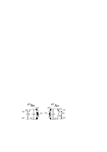
Figure 1: (adapted from letter ) Partial level scheme of ⁶⁷Se and ⁶⁷As, showing the decay of the lowest $9/2^{+}$ state. Energy labels are in keV.

Table 1: Values of B(E1) for the transitions proceeding from the lowest $9/2^{+}$ state in⁶⁷Se and ⁶⁷As, as deduced from lifetimes and M2/E1 ratios, determined in letter .

Nucleus	Eγ	B(E1)	$|(\frac{9}{2}^{+}|\!|\mathcal{M}(E1)|\!|\frac{7}{2}^{-})|$
	[keV]	[$e^{2}$ fm2]	[e fm]
67As	$725$	$1.4\pm 0.4\times 10^{-6}$	$3.7\pm 0.5\times 10^{-3}$
67Se	$717$	$0.4\pm 0.4\times 10^{-6}$	$2.0\pm 2.0\times 10^{-3}$
67As	$319$	$8.3\pm 2.5\times 10^{-6}$	$9.1\pm 1.3\times 10^{-3}$
67Se	$303$	$<1.4(9)\times 10^{-6}$	$<3.7(11)\times 10^{-3}$

II Isovector and isoscalar contributions

In the following calculations, the E1 transition is assumed to take place from an intruder single-particle orbital $j_{I}$ to a normal-party orbital $j_{N}=j_{I}-1$ (or vice-versa). The parent state $a$ will be the lowest intruder, with $J_{a}=j_{I}$ and parity $\bar{\pi}$. A possible daughter state $b$ must have $J_{b}=J_{a}\pm 1$ or $J_{a}$ and parity $\pi=-\bar{\pi}$. Its wave function can contain pairs inside intruder orbitals coupled to zero: in this case, the transition could proceed from a $j_{N}$ orbital present in $a$ to a $j_{I}$ orbital in $b$.

If we expand the wave functions of states $a$ and $b$ in terms of products of the one-body wave function times the core wave function (with the proper fractional parentage coefficients) the only terms of the expansion that contribute to the transition are those having a common core state (of isospin $T_{c}=0$ or 1) for both states $a$ and $b$, and the single-particle orbit changing from $j_{I}$ to $j_{N}$ (with a core state $J_{\mu}^{+}$ of positive parity) or vice-versa (with a core state $J_{\mu}^{-}$ of negative parity):

$$|a;J_{a},M_{a};1/2,T_{3}> =$$

$$\phantom{+}\sum_{\mu}C_{fp}(a|j_{I};\mu,J_{\mu}^{+},T_{c})[\phi(j_{I})\otimes\Phi(\mu,J_{\mu}^{+},T_{c})]^{(J_{a},1/2)}_{M_{a},T_{3}}$$

$$\phantom{\times\Big{[}}+\sum_{\mu}C_{fp}(a|j_{N};\mu,J_{\mu}^{-},T_{c})[\phi(j_{N})\otimes\Phi(\mu,J_{\mu}^{-},T_{c})]^{(J_{a},1/2)}_{M_{a},T_{3}}$$

$$+...$$

$$|b;J_{b},M_{b};1/2,T_{3}> =$$

$$\phantom{+}\sum_{\mu}C_{fp}(b|j_{N};\mu,J_{\mu}^{+},T_{c})[\phi(j_{N})\otimes\Phi(\mu,J_{\mu}^{+},T_{c})]^{(J_{b},1/2)}_{M_{b},T_{3}}$$

$$\phantom{\times\Big{[}}+\sum_{\mu}C_{fp}(b|j_{I};\mu,J_{\mu}^{-},T_{c})[\phi(j_{I})\otimes\Phi(\mu,J_{\mu}^{-},T_{c})]^{(J_{b},1/2)}_{M_{b},T_{3}}$$

$$+...$$

Taking into account the relation, to be used both in ordinary space and in isospin space,

$$([j_{1}\otimes j_{2}]J|\!|U^{(K)}(1)|\!|[j_{1}^{\prime}\otimes j_{2}]J^{\prime})=(-1)^{j_{1}+j_{2}+J^{\prime}+K}\phantom{mm}$$

$$\times\sqrt{(2J+1)(2J^{\prime}+1)}\left\{\begin{array}[]{c c c}j_{1}&J&j_{2}\cr J^{\prime}&j_{1}^{\prime}&K\end{array}\right\}(j_{1}|\!|U^{(K)}|\!|j_{1}^{\prime})\ ,$$ (5)

where $U^{(K)}$ is a tensor operator of rank $K$ acting only on the subspace “1”, we obtain for the reduced matrix element between states $a$ and $b$

$$(b,J_{b},T_{b}|\!|\!|\mathcal{M}_{E}^{(1K)}|\!|\!|a,J_{a},T_{a})=$$

$$\sum_{T_{c}}(-1)^{T_{c}+K+1}\widehat{T}_{a}\widehat{T}_{b}\ \left\{\begin{array}[]{c c c}1/2&T_{b}&T_{c}\cr T_{a}&1/2&K\end{array}\right\}\phantom{m}$$ (8)

$$\times\Big{[}\sum_{\mu}(-1)^{J_{a}+j_{N}+J_{\mu}^{+}+1}\ \widehat{J}_{a}\widehat{J}_{b}\left\{\begin{array}[]{c c c}j_{N}&J_{b}&J_{\mu}^{+}\cr J_{a}&j_{I}&1\end{array}\right\}$$ (11)

$$\phantom{m}\times n\ C_{fp}(a|j_{I};\mu,J_{\mu}^{+},T_{c})\ C_{fp}(b|j_{N};\mu,J_{\mu}^{+},T_{c})$$

$$\phantom{m}\times(j_{N}|\!|\!|\mathcal{M}_{E}^{(1K)}|\!|\!|j_{I})$$

$$+\sum_{\mu}(-1)^{J_{a}+j_{I}+J_{\mu}^{-}+1}\ \widehat{J}_{a}\widehat{J}_{b}\left\{\begin{array}[]{c c c}j_{I}&J_{b}&J_{\mu}^{-}\cr J_{a}&j_{N}&1\end{array}\right\}$$ (14)

$$\phantom{m}\times n\ C_{fp}(a|j_{N};\mu,J_{\mu}^{-},T_{c})\ C_{fp}(b|j_{I};\mu,J_{\mu}^{-},T_{c})$$

$$\phantom{m}\times(j_{I}|\!|\!|\mathcal{M}_{E}^{(1K)}|\!|\!|j_{N})\ \Big{]}\ ,$$ (15)

where $n$ is the number of active nucleons, $\widehat{J}\equiv\sqrt{2J+1}$, and the triple bars indicate a reduced matrix element with respect to ordinary space and to isospin space (with $T_{a}=T_{b}=1/2$). The operator $\mathcal{M}_{E}^{(1K)}$ is now a tensor of rank 1 in the ordinary space and $K=1$ or $0$ in isospin space.
Now,

$$(j_{N}|\!|\!|\mathcal{M}_{E}^{(1K)}|\!|\!|j_{I}) = \!(-1)^{j_{I}-j_{N}}\overline{(j_{I}|\!|\!|\mathcal{M}_{E}^{(1K)}|\!|\!|j_{N})}$$ (16)

$$= +\ (j_{I}|\!|\!|\mathcal{M}_{E}^{(1K)}|\!|\!|j_{N})\phantom{i}.$$

Here, $j_{I}-j_{N}=1$, both single-particle states have isospin 1/2 and the E1 operator is odd under time reversal. We obtain therefore for the reduced matrix element in ordinary space

$$(b,J_{b};T_{b},T_{3}|\!|\mathcal{M}_{E}^{(1K)}|\!|a,J_{a};T_{a},T_{3})=$$ (22)

$$= (-1)^{1/2-T_{3}}\left(\begin{array}[]{c c c}T_{b}&K&T_{a}\cr-T_{3}&0&T_{3}\end{array}\right)(j_{N}|\!|\!|\mathcal{M}_{E}^{(1K)}|\!|\!|j_{I})$$

$$\times(-1)^{K}\sum_{T_{c}=0,1}\mathcal{A}(T_{c})\left\{\begin{array}[]{c c c}1/2&T_{b}&T_{c}\cr T_{a}&1/2&K\end{array}\right\}\ ,$$

where $\mathcal{M}^{(11)}\equiv D_{IV}^{(1)}\vec{\tau}$ and $\mathcal{M}^{(10)}\equiv D_{IS}^{(1)}$ are the isovector and isoscalar part of the single-particle electric dipole operator:

$$(j_{N}|\!|\!|\mathcal{M}_{E}^{(10)}|\!|\!|j_{I}) = (j_{N}|\!|D^{(1)}_{IS}|\!|j_{I})(1/2|\!|1|\!|1/2)\phantom{mm}$$ (23)

$$(j_{N}|\!|\!|\mathcal{M}_{E}^{(11)}|\!|\!|j_{I}) = (j_{N}|\!|D^{(1)}_{IV}|\!|j_{I})(1/2|\!|\vec{\tau}|\!|1/2)$$

and the core-isospin dependent coefficients $\mathcal{A}(T_{c})$ ($T_{c}=0$ or $1$) are

$$\mathcal{A}(T_{c}) = (-1)^{T_{c}}\ 2\widehat{J}_{a}\widehat{J}_{b}$$ (24)

$$\times \Big{[}\sum_{\mu}(-1)^{J_{\mu}^{+}+J_{a}+j_{N}}\left\{\begin{array}[]{c c c}j_{N}&J_{b}&J_{\mu}^{+}\cr J_{a}&j_{I}&1\end{array}\right\}$$

$$\times nC_{fp}(a|j_{I};\mu,J_{\mu}^{+},T_{c})\times C_{fp}(b|j_{N};\mu,J_{\mu}^{+},T_{c})$$

$$+ \sum_{\mu}(-1)^{J_{\mu}^{-}+J_{b}+J_{I}}\left\{\begin{array}[]{c c c}j_{I}&J_{a}&J_{\mu}^{-}\cr J_{b}&j_{N}&1\end{array}\right\}$$

$$\times nC_{fp}(a|j_{N};\mu,J_{\mu}^{-},T_{c})\times C_{fp}(b|j_{I};\mu,J_{\mu}^{-},T_{c})\Big{]}\ .$$

With $T_{a}=T_{b}=1/2$, $T_{c}=0$ or $1$, by inserting the numerical values of the coefficients one obtains

$$(b,J_{b};1/2,T_{3}|\!|\mathcal{M}_{E}^{(11)}|\!|a,J_{a};1/2,T_{3})$$ (31)

$$\phantom{mmm}=\frac{(-1)^{1/2+T_{3}}}{6}\left[\mathcal{A}(1)+3\mathcal{A}(0)\right](j_{I}|\!|D^{(1)}_{IV}|\!|j_{N})$$

$$(b,J_{b};1/2,T_{3}|\!|\mathcal{M}_{E}^{(10)}|\!|a,J_{a};1/2,T_{3})$$ (32)

$$\phantom{mmm}=\frac{1}{2}\left[\mathcal{A}(1)-\mathcal{A}(0)\right](j_{I}|\!|D^{(1)}_{IS}|\!|j_{N})\ .$$

The leading isovector term in the single-particle operator is, in our case,

$$(j_{I}|\!|D^{(1)}_{IV}|\!|j_{N})=\frac{e}{2}<j_{I}|r|j_{N}>(j_{I}|\!|Y^{(1)}|\!|j_{N})$$ (33)

where $Y^{(1)}$ is the spherical harmonic for $\ell=1$.

The different forms of possible isoscalar contributions are discussed in the following sections.

III Higher-order terms after Siegert

It is well known that the usual expression of electric transition amplitudes, deduced from the Siegert’s theorem, is only valid in the long wavelength limit. The complete expression for the electric transition amplitude, taking also into account relativistic corrections, is given by Friar and Fallieros friar :

$$T(E,LM) = \frac{k^{L-1}}{(2L+1)!!}$$ (34)

$$\times\int{\rm d}r^{3}\left[i\sqrt{\frac{L+1}{L}}\dot{\rho}(\vec{r})r^{L}Y^{(L)}_{M}(\hat{r})g_{L}(kr)\right.$$

$$\hskip 11.38109pt\left.+\frac{2k^{2}r}{L+2}\vec{\mu}(\vec{r})\cdot\vec{\mathcal{Y}}^{(L,1)L}_{M}h_{L}(kr)\right]\ ,$$

where $\vec{\mathcal{Y}}^{(L,1)L}_{M}$ is the vector spherical harmonic and

$$g_{L}(z) \approx 1-\frac{Lz^{2}}{2(L+2)(2L+3)}+...$$ (35)

$$h_{L}(z) = -\frac{L+2}{Lz}\frac{\rm d}{{\rm d}z}\left\{z^{-2L}\frac{\rm d}{{\rm d}z}\left[z^{2L+1}g_{L}(z)\right]\right\}\approx 1+...$$

For our purposes, it will be sufficient to consider only the first term after the Siegert limit, as given in the Eqs. (35). We will consider first the part of the integral (34) containing the time derivative of the charge density $\rho=\rho_{0}(\vec{r})\exp(-ikct)$, approximating the nucleus to an ensemble of point-like nucleons:

$$\dot{\rho}=-ikc\rho(\vec{r})\approx-ikc\sum\frac{1+\tau_{3}(i)}{2}e\ \delta(\vec{r}-\vec{r_{i}})\ .$$ (36)

The isovector part of the E1 transition operator is, for a single-particle transition,

$$D_{IV}(E1)\tau_{3}=\frac{\sqrt{2}}{3}\frac{e}{2}kc\ rY^{(1)}(\hat{r})\tau_{3}\ .$$ (37)

To first approximation, the isoscalar part of the transition amplitude only comes from the second term of the series expansion of $g_{L}(kr)$. As we have to deal with a one-body operator, we can easily obtain the amount of this correction with respect to the main (Siegert) term, for each single-particle transition:

$$\frac{\left<\ell_{1},j_{1}|\!|D^{E}_{IS}(E1)|\!|\ell_{2},j_{2}\right>}{\left<\ell_{1},j_{1}|\!|D_{IV}(E1)|\!|\ell_{2},j_{2}\right>}=-\frac{k^{2}}{30}\frac{\left<\ell_{1},j_{1}|r^{3}|\ell_{2},j_{2}\right>}{\left<\ell_{1},j_{1}|r|\ell_{2},j_{2}\right>}\ .$$ (38)

Now we can estimate the numerical value of this ratio for the case of the $A=67$ doublet letter chosen as a suitable benchmark, and for a $g_{9/2}\to f_{7/2}$ transition. With Woods-Saxon radial wavefunctions one obtains

$$\frac{\left<f_{7/2}|(r/R_{0})^{3}|g_{9/2}\right>}{\left<f_{7/2}|r/R_{0}|g_{9/2}\right>}=0.834.$$ (39)

Assuming $R_{0}=1.27A^{1/3}$fm $=5.158$fm:

$$\frac{k^{2}}{30}\ \frac{\left<f_{7/2}|r^{3}|g_{9/2}\right>}{\left<f_{7/2}|r|g_{9/2}\right>} = \frac{1}{30}\ (kR_{0})^{2}\frac{\left<f_{7/2}|(r/R_{0})^{3}|g_{9/2}\right>}{\left<f_{7/2}|r/R_{0}|g_{9/2}\right>}$$ (40)

$$= 1.90\times 10^{-5}(E_{\gamma}[{\rm MeV}])^{2}\ .$$

The evaluation of the second part of Eq. (34) can be easily performed if we substitute the continuous magnetic density $\vec{\mu}(\vec{r})$ with that of an ensemble of point-like nucleons with spin:

$$\vec{\mu}(\vec{r}) = \mu_{n}\sum_{i}\left\{\frac{1+\tau_{3}(i)}{2}\left[\vec{\ell}_{i}+g_{p}\vec{s}_{i}\right]\right.$$ (41)

$$+ \left.\frac{1-\tau_{3}(i)}{2}g_{n}\vec{s}_{i}\right\}\delta(\vec{r}-\vec{r}_{i})$$

$$= \frac{\mu_{n}}{2}\sum\big{\{}\left[\vec{j}_{i}+(g_{p}-1+g_{n})\vec{s}_{i}\right]$$

$$+ \left[\vec{j}_{i}+(g_{p}-1-g_{n})\vec{s}_{i}\right]\tau_{3}(i)\big{\}}\ ,$$

where $\mu_{n}=e\hbar/(2M_{p})$ is the nuclear magneton (and $M_{p}$ the proton mass). On the basis of Eq. (40), we can observe that the magnitude of this term in comparison to the first term of Eq. (34) is given by

$$\frac{k^{2}\mu_{n}}{kec}=\frac{\hbar kc}{2M_{p}c^{2}}\approx 0.53\ 10^{-3}E_{\gamma}[MeV]\ .$$ (42)

Here, we are only interested in the isoscalar part, where the contribution of the term $\vec{s}$ is hindered due to the numerical factor $g_{p}-1+g_{n}\approx 0.76$. The evaluation of the matrix elements of $\vec{s}\cdot\vec{\mathcal{Y}}^{(L,1)L}_{M}$ and $\vec{j}\cdot\vec{\mathcal{Y}}^{(L,1)L}_{M}$ is performed in detail in Appendix A. For our benchmark, corresponding to a $g_{9/2}\to f_{7/2}$ single-particle transition, one obtains

$$\frac{(g_{9/2}|\!|D^{M}_{IS}|\!|f_{7/2})}{(g_{9/2}|\!|D_{IV}|\!|f_{7/2})} \approx -\frac{2\sqrt{2}}{3}\ \frac{k\mu_{n}}{ec}\left[\frac{(g_{p}-1+g_{n})}{\sqrt{6}}-\frac{1}{\sqrt{2}}\right]$$ (43)

$$\approx 2\times 10^{-4}\ (E_{\gamma}[{\rm MeV}])$$

if we assume that the above description of the magnetic density is approximately correct.

For $\gamma$-ray energies around 1 MeV, both correction terms are far too small to justify the observed asymmetries in $A=67$.

IV The Coulomb mixing of wave functions

If one takes into account the level mixing due to the Coulomb interaction $V_{c}$, the wavefunction of a pure eigenstate $|a_{0}>$ of the charge–invariant Hamiltonian is changed into a new one, $|a^{\prime}>$. To first order,

$$|a^{\prime}> = |a_{0}>+\sum_{k}\frac{<a_{k}|V_{c}|a_{0}>}{E(a_{0})-E(a_{k})}|a_{k}>\ ,$$ (44)

where the sum is extended over all states $|a_{k}>$ having the same $J^{\pi}$ as $|a_{0}>$, and which may or may not have the same isospin. The E1 transition matrix element between the modified states $a^{\prime}$, $b^{\prime}$ is, again to first order,

$$<b^{\prime}|\mathcal{M}(E1)|a^{\prime}>=<b_{0}|\mathcal{M}(E1)|a_{0}>\phantom{mmmmmm}$$ (45)

$$\phantom{mmm}+\sum\frac{<a_{k}|V_{c}|a_{0}>}{E(a_{0})-E(a_{k})}<b_{0}|\mathcal{M}(E1)|a_{k}>$$

$$\phantom{mmm}+\sum\frac{<b_{0}|V_{c}|b_{k}>}{E(b_{0})-E(b_{k})}<b_{k}|\mathcal{M}(E1)|a_{0}>$$

$$\phantom{mmm}\equiv<b_{0}|\mathcal{M}(E1)|a_{0}>+<b_{0}|\widetilde{\mathcal{M}}(E1)|a_{0}>\ .$$

It was assumed, here, that the $\mathcal{M}(E1)$ operator is pure isovector. The ensemble of the first-order corrections (shortly indicated as $<b_{0}|\widetilde{\mathcal{M}}(E1)|a_{0}>$) transforms as an even tensor in isospin space. In the $T=1/2$ or $T=0$ subspaces, it can be considered as an induced isoscalar amplitude.

If $T_{3}=0$ and the unperturbed states $a_{0},\ b_{0}$ have the same isospin, the first term of the sum (45) vanishes and only the induced part contributes. Instead, if $T_{3}=\pm 1/2$, the first term is the leading one and the other two are only first-order corrections.

The Coulomb potential can be written as the sum of an isoscalar, an isovector and a rank-2 isotensor term:

$$V_{c} = \frac{1}{2}\sum_{i}\sum_{j\neq i}\frac{e^{2}}{r_{ij}}\frac{1+\tau_{3}(i)}{2}\frac{1+\tau_{3}(j)}{2}$$

$$= \frac{1}{8}\sum_{i}\sum_{j\neq i}\frac{e^{2}}{r_{ij}}\left[1+\frac{1}{3}(\bm{\tau}(i)\cdot\bm{\tau}(j)\ )\right]$$

$$+ \sum_{i}\frac{e}{2}\tau_{3}(i)\sum_{j\neq i}\frac{e}{2}\frac{1}{r_{ij}}$$

$$+ \frac{1}{8}\sum_{i}\sum_{j\neq i}\frac{e^{2}}{r_{ij}}\Big{[}\tau_{3}(i)\tau_{3}(j)-\frac{1}{3}\big{(}\ \bm{\tau}(i)\cdot\bm{\tau}(j)\ \big{)}\Big{]}\ .$$

The isoscalar part can be included in the charge-invariant Hamiltonian. The matrix elements of the isotensor term vanish in the $T=1/2$ subspace. They could contribute to the mixing with a $T=3/2$ state but would produce, in any case, equal effects in two mirror nuclei.

Therefore, any difference between mirror nuclei has to be attributed to the mixing induced by the isovector term $V_{c}^{(1)}$

$$V_{c}^{(1)} = \sum_{i}\frac{e}{2}\tau_{3}(i)\sum_{j\neq i}\frac{e}{2}\frac{1}{r_{ij}}\ ,$$ (47)

where $V_{c}^{(1)}$ is, obviously, a two-body operator. It is possible, however, to approximate its matrix elements with those of a suitable one-body operator (see BM , Eq. 2-104). Actually, the second sum in Eq. (47) corresponds to the Coulomb potential of a system of $A-1$ point-like charges $e/2$ associated to all nucleons $j$ different from the nucleon $i$, and we can approximate it with the electrostatic potential of an uniformly-charged sphere of radius $R$, i.e., for $r<R$

$$\varphi_{c}(r)\equiv\frac{e(A-1)}{2R}\ f_{c}(r/R)\approx\frac{e(A-1)}{2R}\ \frac{3R^{2}-r^{2}}{2R^{2}}\ .$$ (48)

(slightly different forms of the function $f_{c}$ will be considered in the following). With these approximations,

$$V_{c}^{(1)} \approx \sum_{i}\frac{e}{2}\tau_{3}(i)\varphi_{c}(r_{i})$$ (49)

$$= eT_{3}\varphi_{c}(0)-\sum_{i}\frac{e}{2}\tau_{3}(i)[\varphi_{c}(0)-\varphi_{c}(r)]$$

$$\equiv eT_{3}\varphi_{c}(0)+\widetilde{V}_{c}^{(1)}$$

and, for the potential $\varphi_{c}$ of an uniformly charged sphere,

$$\widetilde{V}_{c}^{(1)}=-\frac{e(A-1)}{R^{3}}\sum_{i}\frac{er_{i}^{2}\tau_{3}(i)}{8}\ .\phantom{mm}$$ (50)

The first term of Eq. (49) is diagonal and does not contribute to the mixing. The second term is proportional to the isovector monopole operator

$$\mathcal{M}^{(1)}(E0)=\sum_{i}\frac{e\ r_{i}^{2}\tau_{3}(i)}{2}\ .$$ (51)

This result will be exploited again in Section IV.3.

Actually, the use of a constant charge density inside a sphere to evaluate the electrostatic potential $\varphi_{c}$ is somewhat inconsistent with the Woods-Saxon distribution of matter density assumed to calculate the radial wavefunctions. Moreover, the tails of these wavefunctions extend outside the nuclear radius, in a region where $\varphi_{c}$ would decrease as $1/r$. Calculations of the electrostatic potential for a Woods-Saxon density of charge are given in Appendix B. For small values of $r$ – i.e., as long as the charge density of the Woods-Saxon distribution is substantially constant and equal to that of the sphere – the values of $\widetilde{V}_{c}^{(1)}$ are equal in the two cases, and the differences in the calculated integral are always rather small. To obtain the same charge density at the centre, the radius $R$ of the uniformly charged sphere must take a slightly different value from the parameter $R_{0}$ of the Woods-Saxon distribution. Adopting for the Woods-Saxon parameters the values suggested by Bohr and Mottelson BM , $R_{0}=1.27A^{1/3}$ fm, $a=0.67$ fm, for $A=67$ one obtains $R_{0}=5.158$ fm and $R=5.430$ fm.

The matrix elements of $\widetilde{V}_{c}^{(1)}$ are in any case very small. To produce a sizable mixing of states, it is necessary that the effect be amplified due to some particular conditions. This can happen, in particular, (i) when two levels with equal $J^{\pi}$ are very close in energy or (ii) have very similar wavefunctions, or (iii) when many different levels contribute coherently to the mixing. We will consider these three cases in the following subsections.

IV.1 Close-lying states

The simplest possible case is the mixing of two states which lie close in energy. As an example, we can consider the E1 decay of a given state $a$ (of spin $J_{a}$) towards two states $b_{1},\ b_{2}$ of equal angular momentum $J_{b}$, and rather close in energy. In this case, taking into account only the Coulomb mixing between $b_{1}$ and $b_{2}$ (and neglecting small isoscalar terms in the E1 operator) we obtain up to first order

$$(b_{1}^{\prime},J_{b}|\!|\mathcal{M}(E1)|\!|a,J_{a})=$$ (52)

$$=\!(b_{1},J_{b}\!|\mathcal{M}(E1)|\!|a,J_{a})+\alpha T_{3}(b_{2},J_{b}|\!|\mathcal{M}(E1)|\!|a,J_{a})$$

$$(b_{2}^{\prime},J_{b}|\!|\mathcal{M}(E1)|\!|a,J_{a}\!)=$$ (53)

$$=\!(b_{2},J_{b}|\!|\mathcal{M}(E1)|\!|a,J_{a})-\alpha T_{3}(b_{1},J_{b}|\!|\mathcal{M}(E1)|\!|a,J_{a})\phantom{n}$$

with

$$\alpha T_{3}=<b_{1}|\widetilde{V}_{c}^{(1)}|b_{2}>/\ [E(b_{1})-E(b_{2})]$$ (54)

In fact, as a consequence of the Wigner–Eckart theorem, the matrix element of $\widetilde{V}_{c}^{(1)}$ must be proportional to that of $T_{3}$.

The reduced transition probabilities become, up to first order

$$B(E1;a\to b^{\prime}_{1})=\frac{1}{2J+1}\Big{[}(b_{1},J^{\prime}|\!|\mathcal{M}(E1)|\!|a,J)^{2}$$ (55)

$$+2\alpha T_{3}(b_{1},J_{b}|\!|\mathcal{M}(E1)|\!|a,J_{a})(b_{2},J_{b}|\!|\mathcal{M}(E1)|\!|a,J_{a})\Big{]}$$

$$B(E1;a\to b^{\prime}_{2})=\frac{1}{2J_{a}+1}\Big{[}(b_{2},J_{b}|\!|\mathcal{M}(E1)|\!|a,J_{a})^{2}$$ (56)

$$-2\alpha T_{3}(b_{1},J_{b}|\!|\mathcal{M}(E1)|\!|a,J_{a})(b_{1},J_{b}\!|\mathcal{M}(E1)|\!|a,J_{a})\Big{]}.$$

Hence, the sum of the two reduced strengths,

$$B(E1;a\to b^{\prime}_{1})+B(E1;a\to b^{\prime}_{2})=$$ (57)

$$\frac{1}{2J_{a}+1}\Big{[}(b_{1},J_{b}|\!|\mathcal{M}(E1)|\!|a,J_{a})^{2}+(b_{2},J_{b}|\!|\mathcal{M}(E1)|\!|a,J_{a})^{2}\ \Big{]}$$

is independent of $T_{3}$ and consequently identical in the two mirror nuclei. If one of the two unperturbed transition strengths (either for $a\to b_{1}$ or $a\to b_{2}$) is much smaller than the other, a large percentage difference between mirror values can be found, but only for the weaker transition.

IV.2 Analogue – antianalogue mixing

A second interesting case concerns the mixing between two very similar wavefunctions, as for a pair of analogue – antianalogue states (this would be a very favourable case of the mixing of $T=1/2$ and $T=3/2$ states discussed in patt08 ). Let us consider, as a simple example, the state obtained with the coupling of a $j_{I}=9/2$ nucleon to the lowest state $\phi_{0}$ ($J^{\pi}=0^{+},\ T=1$) of the isospin triplet $A=66$. Isospin $3/2$ states are obtained in the two $|T_{3}|=3/2$ nuclei. In the $|T_{3}|=1/2$ nuclei ⁶⁷As, ⁶⁷Se two independent wavefunctions will result from the coupling, and two pure isospin states can be constructed by proper linear combinations: a $T=3/2$ state $|a_{3}>$, which is the isospin analogue of those in the $|T_{3}|=3/2$ nuclei, and a $T=1/2$ state $|a_{1}>$, sometime referred to as the anti-analogue of them. Here we will give the results for the $T_{3}=+1/2$ nucleus (from which, those for $T_{3}=-1/2$ can be easily deduced by means of the Wigner-Eckart theorem):

$$\left|a_{3}\right> = \big{|}[\phi_{j}(t=1/2)\otimes\Phi_{0}(T_{c}=1)]j,T=3/2\big{>}$$

$$= c_{1}\big{|}\phi_{\pi}(g_{9/2})\ \Phi_{0}(T_{3}=0)\big{>}$$

$$+ c_{2}\big{|}\phi_{\nu}(g_{9/2})\ \Phi_{0}(T_{3}=1)\big{>}$$

$$\left|a_{1}\right> = \big{|}[\phi_{j}(t=1/2)\otimes\Phi_{0}(T_{c}=1)]j,T=1/2\big{>}$$

$$= c_{2}\big{|}\phi_{\pi}(g_{9/2})\ \Phi_{0}(T_{3}=0)\big{>}$$

$$- c_{1}\big{|}\phi_{\nu}(g_{9/2})\ \Phi_{0}(T_{3}=1)\big{>}$$

where, for $T_{3}=+1/2$,

$$c_{1} = (1/2,1/2,1,0\ |\ 3/2,1/2)$$ (60)

$$= -(1/2,-1/2,1,1\ |\ 1/2,1/2)=\sqrt{2/3}$$

and

$$c_{2} = (1/2,-1/2,1,1\ |\ 3/2,1/2)$$ (61)

$$= (1/2,1/2,1,0\ |\ 1/2,1/2)=\sqrt{1/3}.$$

We now use Eqs. (49,50) to approximate the non diagonal part of the isovector Coulomb interaction $V_{C}^{(1)}$ with a one-body operator $\widetilde{V}_{C}^{(1)}$, whose matrix element between analogue and antianalogue states is, for $T_{3}=+1/2$,

$$\left<a_{3}|\widetilde{V}_{C}^{(1)}|a_{1}\right> = \!c_{1}c_{2}\left<\phi_{\pi}\Phi_{0}(1,0)|\widetilde{V}_{C}^{(1)}|\phi_{\pi}\Phi_{0}(1,0)\right>$$ (62)

$$- \!c_{2}c_{1}\left<\phi_{\nu}\Phi_{0}(1,1)|\widetilde{V}^{(1)}_{C}|\phi_{\nu}\Phi_{0}(1,1)\right>$$

$$= \!c_{1}c_{2}\left[\left<\phi|\widetilde{V}^{(1)}_{C}(\pi)|\phi\right>-\left<\phi|\widetilde{V}^{(1)}_{C}(\mu)|\phi\right>\right.$$

$$- \left.\left<\Phi_{0}(1,1)|\widetilde{V}^{(1)}_{C}|\Phi_{0}(1,1)\right>\right]\ .$$

The diagonal matrix element of the isovector operator $\widetilde{V}^{(1)}_{C}$ over the core state $T=1,T_{3}=0$ is zero.

Starting from Eq. (62) and assuming an energy spacing $E(a_{3})-E(a_{1})=\Delta E$, we can now estimate at least the order of magnitude of the mixing coefficient. For $T_{3}=+1/2$,

$$\alpha = \frac{\Big{<}a_{3}\Big{|}\widetilde{V}^{(1)}_{C}\Big{|}a_{1}\Big{>}}{(-\Delta E)}=c_{1}c_{2}\frac{(A-1)e^{2}}{8R\ \Delta E}\Big{[}2\Big{<}g_{9/2}|\frac{r^{2}}{R^{2}}|g_{9/2}\Big{>}$$ (63)

$$- \Big{<}\Phi_{0}(1,1)\Big{|}\sum_{i}\tau_{3}(i)\frac{r_{i}^{2}}{R^{2}}\Big{|}\Phi_{0}(1,1)\Big{>}\Big{]}$$

In the second term, the contributions of a proton and of a neutron in the same orbit cancel one another, due to the opposite eigenvalue of $\tau_{3}$. There are, however, two excess protons in the $T_{3}=1$ core state. If all the radial wavefunctions of active nucleons in the core were equivalent to that of the $j_{I}$ orbit, the second term in the sum of Eq. (63) would exactly cancel the first one. We can expect, therefore, a resulting matrix element substantially smaller than the first term alone, due to the effect of the core term. However, the expectation value of $r^{2}/R^{2}$ in the $j_{I}=g_{9/2}$ orbit is certainly larger than those for the lower orbits in the core. For $A=67$, and with Woods-Saxon wavefunctions, the radial integral of $(r/R)^{2}$ in the $0g_{9/2}$ orbit is 0.7495, while in the normal-party orbits $0f_{7/2}$. $0f_{5/2}$, $1p_{3/2}$ and $1p_{1/2}$ is, respectively, 0.6251, 0.5922, 0.6251, and 0.6359. In Eq. (63), we will use the average of these values, $<r^{2}/R^{2}>=0.6119$, and the above estimate of the matrix element in the $g_{9/2}$ orbit, to evaluate an order of magnitude for the analogue-antianalogue mixing. Numerically, with $c_{1}c_{2}=\sqrt{2}/3$, $A=67$, $R=4.43$fm and assuming $\Delta E\approx 4$ MeV as in ⁵⁹Cu maripuu72 , we obtain $\alpha\approx 0.071$. As the matrix element of the isovector interaction $\widetilde{V}^{(1)}_{C}$ between a state of isospin $3/2$ and a state of isospin $1/2$ is

$$\left<3/2,T_{3}|\widetilde{V}^{(1)}_{C}|1/2,T_{3}\right> = (-1)^{3/2-T_{3}}\left(\begin{array}[]{ccc}3/2&1&1/2\cr-T_{3}&0&T_{3}\end{array}\right)$$ (66)

$$\times (3/2|\!|\widetilde{V}^{(1)}_{C}|\!|1/2)\phantom{mm}$$ (67)

the value of $\alpha$ has equal sign in both nuclei of the doublet.

The E1 transition matrix element from the state $|a_{1}^{\prime}>$ to a given state $|b>$ will be, at the first order,

$$\left<b|\!|\mathcal{M}(E1)|\!|a_{1}^{\prime}\right>=\left<b|\!|\mathcal{M}(E1)|\!|a_{1}\right>+\alpha\left<b|\!|\mathcal{M}(E1)|\!|a_{3}\right>.\phantom{mm}$$ (68)

We assume, for sake of simplicity, that the state $b$ has pure isospin 1/2. If, as we have supposed, the E1 transition proceeds from a $j_{I}=9/2$ to a $j_{N}=7/2$ single-particle state, we can use for the state $|b>$ a fractional parentage expansion in the style of the first line of Eq. (II). But only the terms corresponding to the coupling of a nucleon in the state $j_{N}=7/2$ to the core configuration $\Phi_{0}$ with $J=0,T=1$ can be reached by the E1 transition. We can write the (presumably small) part of the wavefunction of the state $b$ which is relevant for the E1 transition in the form of Eq.(IV.2).

$$\left|b\right> = \left|[\phi_{j}(t=1/2)\otimes\Phi_{0}(T_{c}=1)]j,T=1/2\right>+...$$

$$= c_{2}\left|\phi_{\pi}(f_{7/2})\ \Phi_{0}(T_{3}=0)\right>$$

$$- c_{1}\left|\phi_{\mu}(f_{7/2})\ \Phi_{0}(T_{3}=1)\right>+...$$

Taking into account the effective charges for E1 transition, $\epsilon_{\pi}=1/2$ and $\epsilon_{\nu}=-1/2$, from Eq. (68) we obtain

$$\left(b|\!|\mathcal{M}(E1)|\!|a_{1}^{\prime}\right) = \left[(|c_{2}|^{2}\epsilon_{\pi}+|c_{1}|^{2}\epsilon_{\nu})+\alpha c_{1}c_{2}(\epsilon_{\pi}-\epsilon_{\nu})\right]$$

$$\times (f_{7/2}|\!|erY^{(1)}|\!|g_{9/2})$$

$$=\frac{-1+2\sqrt{2}\ \alpha}{6}(f_{7/2}|\!|erY^{(1)}|\!|g_{9/2})$$

For $T_{3}=\pm 1/2$, using Eq.(66) we obtain the numerical coefficient $(\mp 1+2\sqrt{2}\ \alpha)/6$. In conclusion, the E1 strength in the two mirror transitions is proportional to $(\mp 1+2\sqrt{2}\alpha)^{2}$. The mirror asymmetry in the E1 strength is therefore, approximately,

$$\frac{B(E1,As)-B(E1,Se)}{B(E1,As)+B(E1,Se)}=\frac{4\sqrt{2}\ \alpha}{1+8\alpha^{2}}\approx 0.386$$ (70)

and the ratio $B(E1,As)/B(E1,Se)\approx 2.26$. We note, however, that such a large asymmetry has been obtained for a pure configuration of the analogue and antianalogue states, while the antianalogue strength is usually spread over a number of final states sherr65 , a situation which will strongly reduce the mirror asymmetry in the E1 strength. A detailed shell-model investigation would possibly elucidate the role of the analogue-antianalogue mixing in the E1 asymmetry between mirror nuclei, as the analogue and the antianalogue states can be described in the same shell-model space.

IV.3 Coherent enhancement of induced isoscalar E1

The Coulomb mixing discussed in the previous subsections involves states belonging to the same set of shell-model orbits necessary for the (unperturbed) parent and daughter state of the E1 transitions (presumably limited to two major shells). However, it is well known that a comparatively large contribution to the isospin mixing comes from states outside this model space, as those belonging to the giant isovector monopole resonance colo95 . Obviously, the mixing with any of these higher-lying states, induced by the isovector part of the Coulomb interaction, is expected to be very small. The combined effect of many higher-lying states on the E1 transition amplitude can however become appreciable if their individual contributions combine coherently. We shall see how this can be the case.

We have seen (Eqs. 49,50) that the non-diagonal isovector part of the Coulomb interaction $V_{c}$ can be approximated with a one-body operator $\widetilde{V}_{C}^{(1)}$, having the same form of the isovector monopole operator $\mathcal{M}^{(1)}(E0)$. Therefore, it is a sensible approximation bini ; bizzeti to consider in the ensemble of states $a_{k}$, $b_{k}$ (with $k\neq 0$) of Eqs. (44,45) only those of the isovector monopole resonances built over $a_{0}$ and $b_{0}$, and to use the mean excitation energy $\Delta E_{a}$ (or $\Delta E_{b}$) of the giant resonance over the state $a_{0}$ (or $b_{0}$) in the place of those of individual states. In this case, Eq. (45) becomes

$$<b^{\prime}|\mathcal{M}(E1)|a^{\prime}>=$$ (71)

$$=<b_{0}|\mathcal{M}(E1)|a_{0}>+<b_{0}|\widetilde{\mathcal{M}}(E1)|a_{0}>\ ,$$

where

$$<b_{0}|\widetilde{\mathcal{M}}(E1)|a_{0}>$$

$$\approx \frac{-1}{\Delta E_{a}}\sum<b_{0}|\mathcal{M}(E1)|a_{k}><a_{k}|V_{c}|a_{0}>$$

$$+ \frac{-1}{\Delta E_{b}}\sum<b_{0}|V_{c}|b_{k}><b_{k}|\mathcal{M}(E1)|a_{0}>\ .$$

We are only interested in the isoscalar part of $\mathcal{M}(E1)$, which results from the isovector part $V_{c}^{(1)}$ of the Coulomb interaction. Approximating the non diagonal part of $V_{c}^{(1)}$ with the one-body potential of Eq. (50), the closure approximation gives

$$\sum<b_{0}|\widetilde{V}^{(1)}_{c}|b_{k}><b_{k}|\mathcal{M}(E1)|a_{0}>$$

$$\approx <b_{0}|\widetilde{V}^{(1)}_{c}\ \mathcal{M}(E1)|a_{0}>$$

$$\sum<b_{0}|\mathcal{M}(E1)|a_{k}><a_{k}|\widetilde{V}^{(1)}_{c}|a_{0}>$$

$$\approx <b_{0}|\mathcal{M}(E1)\ \widetilde{V}^{(1)}_{c}|a_{0}>\ .$$

and therefore (as $\mathcal{M}(E1)$ and $\widetilde{V}^{(1)}_{c}$ commute)

$$<b_{0}|\widetilde{\mathcal{M}}^{(0)}(E1)|a_{0}> \approx 2\frac{<b_{0}|\mathcal{M}(E1)\widetilde{V}_{c}^{(1)}|a_{0}>}{(-\Delta E_{0})}\phantom{mmm}$$ (74)

where we have assumed $\Delta E_{a}\approx\Delta E_{b}\Rightarrow\Delta E_{0}$.

$$<b_{0}|\widetilde{\mathcal{M}}^{(0)}(E1)V_{c}^{(1)}|a_{0}>\approx\ \frac{2}{(-\Delta E_{0})}\ \times$$ (75)

$$\Big{<}b_{0}\Big{|}\sum_{i}\frac{e}{2}r_{i}Y^{(1)}(\hat{r}_{i})\tau_{3}(i)\sum_{j}\frac{e}{2}[\varphi_{c}(r_{j})-\varphi_{c}(0)]\tau_{3}(j)\Big{|}a_{0}\Big{>}\phantom{n}$$

$$\equiv \ \Big{<}b_{0}\Big{|}\widetilde{\mathcal{M}}^{(0)}_{1-b}+\widetilde{\mathcal{M}}^{(0)}_{2-b}\Big{|}a_{0}\Big{>}$$

where $\widetilde{\mathcal{M}}^{(0)}_{1-b}$ is the one-body operator resulting from the term with $j=i$ in the second sum, and $\widetilde{\mathcal{M}}^{(0)}_{2-b}$ is a two-body operator resulting from all other terms. As $\tau_{3}^{2}=1$, the first term is

$$\widetilde{\mathcal{M}}^{(0)}_{1-b}=\frac{1}{\Delta E_{0}}\sum_{i}\ e[\varphi_{c}(0)-\varphi_{c}(r_{i})]\ \frac{e}{2}r_{i}Y^{(1)}(\hat{r}_{i})$$ (76)

With the expression of $\varphi_{c}$ corresponding to the uniformly charged sphere, given in Eq. (48) (and extrapolated also for $r>R$) one obtains for the one-body operator

$$\widetilde{\mathcal{M}}^{(0)}_{1-b}\equiv C\ \sum_{i}\frac{r_{i}^{3}}{R^{2}}\frac{e}{2}\ Y^{(1)}(\hat{r}_{i})$$ (77)

which has the same structure as the one coming from the second-order term in the series expansion of Eq. (34), with a different coefficient,

$$C=+(A-1)e^{2}/\ (8R\Delta E_{0}).$$ (78)

An alternative calculation using a Woods-Saxon charge distribution is reported in the Appendix B.

As the one-body operator (74) is isoscalar, its matrix elements can be expressed in the form anticipated in Eq. (32):

$$\Big{(}b,J_{b};\frac{1}{2},T_{3}\Big{|}\!\Big{|}\sum_{i}\frac{e}{2}\ \frac{r_{i}^{2}}{R^{3}}\ r_{i}Y^{(1)}(\hat{r}_{i})\Big{|}\!\Big{|}a,J_{a};\frac{1}{2},T_{3}\Big{)}$$

$$\hskip 28.45274pt=\frac{1}{2}\left[\mathcal{A}(1)-\mathcal{A}(0)\right]\frac{e}{2}\ \Big{(}j_{N}\Big{|}\!\Big{|}r\ Y^{(1)}(\hat{r})\Big{|}\!\Big{|}j_{I}\Big{)}$$

$$\hskip 42.67912pt\times\frac{\left<j_{N}|(r/R)^{3}|j_{I}\right>}{\left<j_{N}|(r/R)|j_{I}\right>}$$ (79)

Again, we can evaluate the numerical results for our benchmark doublet. For $A=67$, we assume $R=5.30$ fm. The energy difference is $\Delta E_{0}\approx 20$ MeV in ⁶⁰Ni (according to nakayama ). As $\Delta E_{0}$ is expected to scale as $A^{-1/3}$ colo95 , we assume $\Delta E_{0}\approx 19.3$ MeV for $A=67$. With these assumptions, the numerical value of the adimensional coefficient $C$ in Eq. (78) is $C=0.116$. For the ratio of radial integrals (last factor of Eq. (IV.3)), with the radial wavefunctions corresponding to the Woods-Saxon potential one obtains $\left<g_{9/2}|(r/R)^{3}|f_{7/2}\right>/\left<g_{9/2}|r/R|f_{7/2}\right>=0.752$.

It remains to consider the two-body term (second term of Eq. (75)). Again, we can use the fractional parentage expansion of Eqs. (II, II). Here, however, the tensor operator is the product of two factors: a vector isovector term acting on the single-particle state and a scalar isovector one acting on the core state. The product $\tau_{3}(i)\tau_{3}(j)$ contains an isoscalar and an isotensor part:

$$\tau_{3}(i)\tau_{3}(j) = \Big{[}\tau_{3}(i)\tau_{3}(j)-\ \frac{1}{3}\ \big{(}\vec{\tau}(i)\cdot\vec{\tau}(j)\big{)}\Big{]}$$ (80)

$$+ \frac{1}{3}\ \big{(}\vec{\tau}(i)\cdot\vec{\tau}(j)\big{)}$$

but only the isoscalar is effective if the states $a_{0}$ and $b_{0}$ have $T=1/2$. To evaluate the reduced matrix element for the isoscalar part of the two-body operator

$$\widetilde{\mathcal{M}}^{(0)}_{2-b} = \frac{e^{2}}{6\Delta E_{0}}\sum_{i}r_{i}Y^{(1)}(\hat{r}_{i})$$

$$\times \Big{(}\vec{\tau}(i)\cdot\sum_{j\neq i}\vec{\tau}(j)[\varphi(0)-\varphi_{c}(r_{j})]\Big{)}\phantom{mmm}$$

we can use the standard relations of tensor algebra for the matrix elements of tensor products to obtain the reduced matrix element (in ordinary space):

$$\Big{(}b_{0};J_{b};1/2,T_{3}\Big{|}\!\Big{|}\widetilde{\mathcal{M}}^{(0)}_{2-b}\Big{|}\!\Big{|}a_{0};J_{a},1/2,T_{3}\Big{)}$$ (84)

$$= \frac{e}{2}\big{(}j_{N}|\!|rY^{(1)}(\hat{r})|\!|j_{I}\big{)}$$

$$\times \ \frac{C}{\sqrt{3}}\ \sum_{T_{c},T_{c}^{\prime}}(-1)^{T_{c}+1}\left\{\begin{array}[]{ccc}1/2&T_{c}&1/2\cr T_{c}^{\prime}&1/2&1\end{array}\right\}$$

$$\times \Bigg{[}\sum_{\mu,\mu^{\prime}}(-1)^{j_{N}+J_{a}+J_{\mu}^{+}+1}\frac{\widehat{J}_{a}\widehat{J}_{b}}{\widehat{J}^{+}_{\mu}}\left\{\begin{array}[]{ccc}J_{b}&j_{N}&J_{\mu}^{+}\cr j_{I}&J_{a}&1\end{array}\right\}\times$$

$$\phantom{\times}\ C_{fp}(a|j_{I};\mu,J^{+}_{\mu},T_{c})\ C_{fp}(b|j_{N};\mu^{\prime},J^{+}_{\mu},T_{c}^{\prime})$$

$$\phantom{\times}\times\big{(}\mu,J^{+}_{\mu},T_{c}|\!|\!|\sum\frac{r_{j}^{2}}{R^{2}}\vec{\tau}(j)|\!|\!|\mu^{\prime},J^{+}_{\mu},T_{c}^{\prime}\big{)}$$

$$+\sum_{\mu,\mu^{\prime}}(-1)^{j_{I}+J_{a}+J_{\mu}^{-}+1}\frac{\widehat{J}_{a}\widehat{J}_{b}}{\widehat{J}^{-}_{\mu}}\left\{\begin{array}[]{ccc}J_{b}&j_{I}&J^{-}_{\mu}\cr j_{N}&J_{a}&1\end{array}\right\}\times$$

$$\phantom{\times}\ C_{fp}(a|j_{N};\mu,J^{-}_{\mu},T_{c})\ C_{fp}(b|j_{I};\mu^{\prime},J^{-}_{c},T_{c}^{\prime})$$

$$\phantom{\times}\times\big{(}\mu,J^{-}_{\mu},T_{c}|\!|\!|\sum\frac{r_{j}^{2}}{R^{2}}\vec{\tau}(j)|\!|\!|\mu^{\prime},J^{-}_{\mu},T_{c}^{\prime}\big{)}\ \Bigg{]}$$

as $J_{\mu^{\prime}}=J_{\mu}$. As the $\widetilde{\mathcal{M}}_{2-b}^{(0)}$ operator transforms as a scalar in isospin space, its matrix elements have the same sign in both nuclei of the isospin doublet.

The parent state can have $T=0$ or 1, and in principle we have to consider both diagonal and non-diagonal matrix elements (in the parent-state variables) of the isovector operator $\sum(r_{j}^{2}/R^{2})\ \vec{\tau}(j)$. Obviously, its matrix elements vanish when $T$ or $T^{\prime}$ is equal to zero. Otherwise, we can use again a fractional parentage expansion. Only terms having the same parent can contribute to the matrix element and, in addition, the one-body operator has non-diagonal terms only between single-particle states (with equal $j^{\pi}$) differing by at least two units of the principal quantum number: i.e., it does not possess non-diagonal matrix elements inside our model space. As for the diagonal ones, shells (or sub-shells) completely filled with protons and neutrons do not contribute to the sum, as they necessarily have $T=0$. If the valence nucleons are all in the same subshell (or, approximately, in subshells with similar $<(r_{j}/R)^{2}>\approx<(r/R)^{2}>_{v}$), the integral over the radial coordinates can be factorised, $\sum\vec{\tau}(i)=2\vec{T}$, and only the diagonal terms with $\mu^{\prime}=\mu$ survive. Therefore, the matrix element takes the form

$$\big{(}\mu,J_{\mu},T_{c}|\!|\!|\sum_{j}(r_{j}^{2}/R^{2})\vec{\tau}(j)|\!|\!|\mu^{\prime},J_{\mu},T_{c}^{\prime}\big{)}$$

$$\approx <(r/R)^{2}>_{v}\ \big{(}J_{\mu}|\!|1|\!|J_{\mu}\big{)}\ \big{(}T_{c}|\!|2\vec{T}|\!|T_{c}^{\prime}\big{)}\ \delta_{\mu,\mu^{\prime}}$$

where $<(r/R)^{2}>_{v}$ is the average over active valence nucleons, and $\big{(}J_{\mu}|\!|1|\!|J_{\mu}\big{)}=\widehat{J}_{\mu}$. For $T_{c}=T_{c}^{\prime}=1$, $(T_{c}|\!|\vec{T}|\!|T_{c})=\sqrt{T_{c}(T_{c}+1)(2T_{c}+1)}=\sqrt{6}$. By comparing the result with Eq. (24), we obtain approximately (as the first 6-J coefficient has the value $-1/3$):

$$\Big{(}b_{0};J_{b};1/2,T_{3}\Big{|}\!\Big{|}\widetilde{\mathcal{M}}_{2-b}^{(0)}\Big{|}\!\Big{|}a_{0};J_{a},1/2,T_{3}\Big{)}$$ (92)

$$\approx -C\ \frac{2}{3}\ \mathcal{A}(1)\frac{e}{2}\big{(}j_{N}|\!|rY^{(1)}(\hat{r})|\!|j_{I}\big{)}\left<(r/R)^{2}\right>_{v}$$

Actually, the expectation values of $r^{2}/R^{2}$ for the different orbitals of the $pf$ shell (estimated with Woods-Saxon wavefunctions) do not differ more than $3\%$ from their average value 0.615, as we obtain in Appendix B. By using this average value, one obtains for the numerical coefficient of the 2-body term $(2/3)\left<(r/R)^{2}\right>_{v}=0.410$. As this value is not negligible in comparison to that of the 1-body term (0.752), a sizable quenching of the isoscalar transition amplitude corresponding to the 1-body term results from the negative interference of the 2-body term. A similar effect is found for the E1 transitions with $\Delta T=0$ in the $N=Z$ nuclei bini . However, in the present case the quenching only concerns the parent $T=1$ term. As the parent $T=0$ term of Eq. (IV.3) has no counterpart in the 2-body matrix element, its contribution remains unaltered.

If we assume that the most important contribution to the asymmetry is due to the effect of coherent mixing, as approximated in this paragraph, we obtain

$$\epsilon(T_{3}) \equiv \frac{(b,7/2^{-};1/2,T_{3}|\!|\widetilde{\mathcal{M}}_{E}^{(10)}|\!|a,9/2^{+};1/2,T_{3})}{(b,7/2^{-};1/2,T_{3}|\!|\mathcal{M}_{E}^{(11)}|\!|a,9/2^{+};1/2,T_{3})}$$

$$= (-1)^{1/2+T_{3}}\ 3C\ \frac{\left<j_{N}|(r/R)^{3}|j_{I}\right>}{\left<j_{N}|r/R|j_{I}\right>}\times\frac{\eta\mathcal{A}(1)-\mathcal{A}(0)}{\mathcal{A}(1)+3\mathcal{A}(0)}\ ,$$

where the quenching factor $\eta$ takes into account the negative interference with the two-body term of Eq. (75).

Equation (IV.3) only gives an approximate estimate of the effect, due to the many simplifying assumptions (notably, the closure approximation) that have been introduced to obtain this result. Moreover, inclusion in the model space of other orbitals of the upper major shell (as discussed in Appendix C) would somewhat alter this result. However, it could be instructive to evaluate some numerical results, also in the limited space considered, to show that the coherent mixing with the IVGMR can explain the large values of the E1 asymmetries observe in our example of the $A=67$ doublet, while the simplest processes discussed in the previous sections were not able to do.

With the above estimate, $\eta=(0.752-0.410)/0.752=0.458$, and the asymmetry ratio for the mirror E1 strengths is

$$\mathcal{R} \equiv \frac{B(E1,T_{3}=-1/2)}{B(E1,T_{3}=+1/2)}=\left[\frac{1+\epsilon^{-}}{1-\epsilon^{-}}\right]^{2}\ ,$$ (94)

where we have put $\epsilon^{-}\equiv\epsilon(-1/2)=-\epsilon(+1/2)$. Now, to obtain a more accurate estimate one should know the ratio $\mathcal{A}(0)/\mathcal{A}(1)$, which in turn depends on the $C_{fp}$ coefficients.

The relative sign of $\mathcal{A}(0)$ and $\mathcal{A}(1)$ depends on the combined effect of all terms in the sum of Eq. (24). However, we can notice that each of them contains a factor $(-1)^{T}$. If any of these terms dominates, the relative sign of $\mathcal{A}(0)$ and $\mathcal{A}(1)$ is well defined and negative. Actually, this is very probably the case also under somewhat broader conditions. Most probably, the second line of Eq. (24) (corresponding to negative–parity parents) is only a small correction in comparison to the first one. Let us consider, from now on, the numerical values corresponding to the $A=67$ doublet. We can note that the expression

$$(-1)^{J}\ \left\{\begin{array}[]{c c c}9/2&9/2&J\cr 7/2&7/2&1\end{array}\right\}$$ (97)

has always the same (negative) sign for all $J$ values (from 0 to 7) and its value changes very slowly as long as $J\leq 3$. Therefore, unless the parentage coefficients have a very singular behaviour, the relative sign is determined only by the factor $(-1)^{T}_{c}$ (see also Eq. (II)).

To obtain just an order-of-magnitude estimate of the expected effect, we could evaluate the asymmetry in the $A=67$ doublet, for two limiting cases in which one of the two coefficients $\mathcal{A}(1)$ and $\mathcal{A}(0)$ is negligible in comparison to the other. Neglecting $\mathcal{A}(1)$ one obtains $\epsilon^{-}\approx-0.753C\approx-0.0872$ and the asymmetry ratio $\mathcal{R}\approx 0.705$.

Taking into account also $\mathcal{A}(1)$ would bring to smaller asymmetry (larger $\mathcal{R}$) if $\mathcal{A}(1)$ and $\mathcal{A}(0)$ have the same sign, but can also result in a larger asymmetry if – as it is most probable – they have opposite sign. If, instead, $\mathcal{A}(0)$ is negligible in comparison to $\mathcal{A}(1)$, $\epsilon^{-}$ is positive and its value depends on the coefficient $\eta$, which takes into account the negative interference of the core terms. With $\eta=0.458$, for $\mathcal{A}_{0}\ll\mathcal{A}_{1}$ one obtains $\epsilon^{-}\approx+0.120$ and $\mathcal{R}\approx 1.62$. Again, a larger asymmetry could be obtained if also a contribution from $\mathcal{A}_{0}$ (having opposite sign) is included.

These results do not change appreciably if one assumes a charge distribution of Woods-Saxon shape (Appendix B): one obtains $\eta=0.445$; for $\mathcal{A}_{1}\ll\mathcal{A}_{0}$ $\epsilon^{-}\approx-0.0852$ and $\mathcal{R}\approx 0.710$; for $\mathcal{A}_{1}\gg\mathcal{A}_{0}$, $\epsilon^{-}\approx+0.116$ and $\mathcal{R}\approx=1.58$.

A last comment concerns the expected sign of $\epsilon^{-}$. If the dominant term in the Eq. (IV.3) is the one with $T=1$ parent, $\epsilon^{-}>0$ and the reduced strength should be larger in the nucleus with $N=Z+1$, for all transitions between $g_{9/2}$ and $f_{7/2}$. The opposite is true if the $T=0$ parent dominates. Again, qualitative considerations can help in predicting the relative importance of the two terms. It is likely, in fact, that one of the most important parents be the lowest $J=0$. Now, if $A=4n+1$, the lowest $J=0$ parent state is the ground state of the even even self-conjugate nucleus with $A-1$ nucleons. Instead, if $A=4n-1$ (as in the case ⁶⁷As – ⁶⁷Se), the selfconjugate parent nucleus is odd-odd and the lowest $J=0$ parent has $T=1$. If this consideration is correct, the predicted sign of the asymmetry is consistent with the experimental results in the $A=67$ mirror pair.

V Conclusions

It seems worth summarising the results obtained for the different processes which could, in principle, produce an asymmetry in the E1 transition strength, as observed in the case of the ⁶⁷As $-\ ^{67}$Se mirror pair. Higher-order terms, either of “electric” or “magnetic” origin, usually excluded from calculations by the approximation linked to the Siegert’s theorem, in the case considered are three orders of magnitude lower than the leading one. We note that these corrections apply to the transition operator and not to the level wavefunctions. Therefore, as long as – as it was assumed here – most of the shell-model terms contributing to the E1 transition involve the same pair of single-particle states, the same combination of fractional parentage coefficients is involved for both the isoscalar and the isovector term. Thus if the isovector term is hindered as a consequence of accidental cancellation, a similar hindrance factor can be expected also to the isoscalar, leaving the ratio almost unchanged. Only meson currents, neglected in our approximate estimation of the magnetic term, could break, to some extent, the above conclusion.

The Coulomb interaction, mixing in a different way the level wavefunctions in the two mirror nuclei, is presumably at the origin of the observed asymmetries. Its effect could be enhanced when a pair of levels having equal $J^{\pi}$ lie, accidentally, close together. E.g., this could have been the case for the two $7/2^{-}$ levels lying between 640 and 1100 keV in ⁶⁷As and ⁶⁷Se. However, if the asymmetry originated uniquely from the mixing between the two daughter levels, the total sum of the reduced strengths of the E1 transitions feeding these levels ought to be equal in the mirror nuclei, in contrast with the experimental evidence.

The Coulomb mixing could also be enhanced if it took place between states with two “very similar” wavefunctions. In Section IV.2 we considered an hypothetical mixing between a “isospin analogue” state and its corresponding “antianalogue”. In the case of mass $A=67$, this mixing would lead to an asymmetry similar in size to the observed effect. It would also give the right sign for the asymmetries. However, this would only happen if our $T=1/2,J^{\pi}=9/2^{+}$ state would be the exact antianalogue of the lowest $T=3/2$ state with the same $J^{\pi}$, while some spread of the antianalogue strength among different levels is expected also in this region of nuclei Fodor76 ; Maripuu70 .

The effects of Coulomb mixing considered thus far only involved states in the same Hilbert subspace needed to describe the parent and daughter states of the E1 transition: in the simplest case, a full major shell and at least one particle-hole excitation to the next major shell. A shell-model calculation in this Hilbert space could treat, on the same footing, both the regular (isovector) part of the E1 transition amplitude and the “induced-isoscalar” term originating from the mixing. In such a calculation, the isovector part of the two-body Coulomb interaction could be added to the empirical residual interactions, which could also include the symmetry-violating part necessary to account for the Coulomb Energy Differences Lenzi .

Finally, we have considered the possible effect of mixing with states outside the truncated shell-model space, as those belonging to the Giant Isovector Monopole Resonances. With the approximations discussed in Section IV.3, this effect could also be expressed in a form that could be treated in the truncated space, if the mean excitation energy of the monopole resonance were at least approximately known.

A shell-model calculation in such a restricted basis could therefore be able to identify the origin of the observed asymmetry in E1 transition strengths. At the moment, the coherent contribution of states belonging to the Giant Isovector Monopole resonance appears as the most probable candidate.

Appendix A Evaluation of the reduced matrix elements for the magnetic term

Here we evaluate the reduced matrix elements of the operators entering in the second line of Eq. (34), between single particle states $\ell_{1},j_{1}$ and $\ell_{2},j_{2}$. To this purpose, the following property talmi of vector spherical harmonics is exploited:

$$\vec{\mathcal{Y}}^{(L,1)J}_{M}\cdot\vec{v}=\left[Y^{(L)}\otimes v^{(1)}\right]^{(J)}_{M},$$ (98)

where $\vec{v}$ is a generic vector. Here the cases $\vec{v}=\vec{s}$ and $\vec{v}=\vec{j}$ are considered.
In the first case, the reduced matrix element of the tensor product can be obtained easily, because $s$ and $Y^{(L)}$ operate on different Hilbert spaces

$$\left(\ell_{1},J_{1}|\!|\left[Y^{(L)}\otimes s^{(1)}\right]^{(J)}|\!|\ell_{2},J_{2}\right)$$ (99)

$$= \widehat{J}_{1}\widehat{J}\widehat{J}_{2}\left\{\begin{array}[]{ccc}\ell_{1}&1/2&J_{1}\cr\ell_{2}&1/2&J_{2}\cr L&1&J\end{array}\right\}\left(\ell_{1}|\!|Y^{(L)}|\!|\ell_{2}\right)\left(1/2|\!|s^{(1)}|\!|1/2\right)$$ (103)

where $J=L$ and $\left(1/2|\!|s^{(1)}|\!|1/2\right)=\sqrt{3/2}$. The relation

$$\left(\ell_{1},J_{1}|\!|Y^{(L)}|\!|\ell_{2},J_{2}\right)=(-1)^{J_{2}+\ell_{1}+L+1/2}$$ (104)

$$\times \frac{\sqrt{3}}{2}\widehat{J}_{1}\widehat{J}_{2}\left\{\begin{array}[]{c c c}J_{1}&J_{2}&L\cr\ell_{2}&\ell_{1}&1/2\end{array}\right\}\left(\ell_{1}|\!|Y^{(L)}|\!|\ell_{2}\right)$$ (107)

can be exploited to express the result in function of $\left(\ell_{1},J_{1}|\!|Y^{(L)}|\!|\ell_{2},J_{2}\right)$ as in Eq. (33):

$$\left(\ell_{1},J_{1}|\!|\left[Y^{(L)}\otimes s^{(1)}\right]^{(L)}|\!|\ell_{2},J_{2}\right)$$ (108)

$$= (-1)^{J_{2}+\ell_{1}+L+1/2}\ \sqrt{2}\ \widehat{L}\ \left\{\begin{array}[]{ccc}\ell_{1}&1/2&J_{1}\cr\ell_{2}&1/2&J_{2}\cr L&1&L\end{array}\right\}$$ (115)

$$\phantom{mm}\times\left\{\begin{array}[]{c c c}J_{1}&J_{2}&L\cr\ell_{2}&\ell_{1}&1/2\end{array}\right\}^{-1}\left(\ell_{1},J1|\!|Y^{(L)}|\!|\ell_{2},J_{2}\right)$$

The second case is not so simple, because the operators $j$ and $Y^{(L)}$ do not commute, so that the symmetrised form of the operator must be employed. Furthermore, they operate on the same Hilbert space, but one can exploit the fact that $\vec{j}$ has no matrix elements between different single-particle states to obtain:

$$\frac{1}{2}\ \left(\ell_{1},J_{1}|\!|\left[Y^{(L)}\otimes j^{(1)}\right]^{(J)}+\left[j^{(1)}\otimes Y^{(L)}\right]^{(J)}|\!|\ell_{2},J_{2}\right)$$ (118)

$$= \frac{1}{2}\left(\ell_{1},J_{1}|\!|Y^{(L)}|\!|\ell_{2},J_{2}\right)\ (-1)^{J_{1}+J+J_{2}}\widehat{J}$$

$$\times \left[\left\{\begin{array}[]{ccc}1&L&J\cr J_{2}&J_{1}&J_{2}\end{array}\right\}\left(J_{2}|\!|j^{(1)}|\!|J_{2}\right)\right.$$

$$+ \left.\left\{\begin{array}[]{ccc}L&1&J\cr J_{1}&J_{2}&J_{1}\end{array}\right\}\left(J_{1}|\!|j^{(1)}|\!|J_{1}\right)\right]$$ (121)

where $(j|\!|j^{(1)}|\!|j)=\sqrt{j(j+1)(2j+1)}$.

In the present case, $L=J=1,\ \ell_{1}=4,\ J_{1}=9/2$, $\ell_{2}=3,\ J_{2}=7/2$. With these numerical values, the coefficients of the reduced matrix element of $Y^{(L)}$ in the Eqs. (108, 118). are, respectively, $\sqrt{1/6}$ and $-\sqrt{1/2}$.

Appendix B Radial wavefunctions and Coulomb potential with a Woods-Saxon distribution

The radial wavefunctions have been calculated assuming a Woods-Saxon potential plus spin-orbit:

$$V(r) = \left[V_{0}+V_{s}\vec{\ell}\cdot\vec{s}\ \frac{r_{0}^{2}}{r}\ \frac{\rm d}{\rm dr}\right]\ \frac{1}{1+e^{(r-R_{0})/a}}$$ (122)

with the values of the constants consistent with Bohr and Mottelson BM : $V_{0}=-51$ MeV, $V_{s}=22$ MeV, $R_{0}=r_{0}~{}A^{(1/3)}$, $r_{0}=1.27$ fm and $a=0.67$ fm.

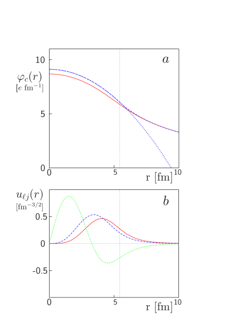
Figure 2: (color online) $a$: electrostatic potential for uniformly charged sphere (dashed) and with a Woods-Saxon charge distribution for $A=67$ (continuous line). The dotted line shows the continuation outside the sphere of the expression for the uniform distribution (dashed curve) in the internal region. $b$: examples of radial wavefunctions for the Woods-Saxon potential ($+$ spin-orbit) with the parameters suggested in BM : $0g_{9/2}$ (continuous line), $0f_{5/2}$ (dashed), $1p_{1/2}$ (dotted). The vertical dotted line corresponds to the value of the nuclear radius $R$.

For a consistent evaluation of Coulomb interactions, one needs the average electrostatic potential $\varphi_{c}(r)$ of a distribution of $A-1$ point charges $e/2$, which will be approximated with a continuous charge distribution having a Woods-Saxon shape:

$$\rho_{e}(r)=\frac{\rho_{0}}{1+e^{\frac{r-R_{0}}{a}}}$$ (123)

where

$$\rho_{0}=(A-1)\frac{e}{2}\ \left[\int\frac{1}{1+e^{\frac{r-R_{0}}{a}}}\ 4\pi r^{2}{\rm d}r\right]^{-1}$$ (124)

With the condition that $\varphi_{c}(r)\to 0$ for $r\to\infty$, we obtain

$$\varphi_{c}(r)\equiv\rho_{0}=\int_{r}^{\infty}\frac{{\rm d}y}{y^{2}}\int_{0}^{y}\frac{\rho_{0}}{1+e^{\frac{x-R_{0}}{a}}}\ x^{2}\ {\rm d}x$$ (125)

This integral has been evaluated numerically, for $A=67$, with the parameter values suggested in BM . In fig.2, the result is compared with the potential of an uniformly charged sphere of charge density equal to $\rho_{0}$ and total charge $(A-1)e/2$. The radius $R$ of the sphere is determined by the condition

$$\frac{4\pi}{3}R^{3}=\frac{(A-1)e}{2\rho_{0}}=\int_{0}^{\infty}\frac{1}{1+e^{\frac{r-R}{a}}}\ 4\pi r^{2}{\rm d}r$$ (126)

To simplify the comparison of the results, $\varphi_{c}(r)$ is expressed in terms of the adimensional function $f_{c}(r/R)$:

$$\varphi_{c}(r)\equiv\frac{(A-1)e}{4R}f_{c}(r/R)\ ,$$ (127)

and we define $\Delta f_{c}(r)=f_{c}(0)-f_{c}(r)$. For the (extrapolated) potential of the uniformly-charged sphere, one obtains $\Delta f_{c}(r)=(r/R)^{2}$. One must now calculate the matrix elements of the operators $\widetilde{\mathcal{M}}_{1-b}^{(0)}$ and $\widetilde{\mathcal{M}}_{2-b}^{(0)}$ defined in Section IV.3. For the one-body term, we consider the ratio

$$\frac{\left<f_{7/2}|(r/R)f_{c}(r/R)|g_{9/2}\right>}{\left<f_{7/2}|r/R|g_{9/2}\right>}$$ (128)

while for the two-body term (and also for the calculations of Section IV.2), it is sufficient to evaluate the diagonal matrix elements of $f_{c}(r/R)$

By numerical integration, with the parameters of BM one obtains the values of the necessary integrals reported in the last column of Table 2. In the other columns, the corresponding values are calculated, with the Woods-Saxon wavefunctions, for the potential of the uniformly charged sphere and for the extrapolation of the inner potential outside the sphere (dotted line in Fig. 2$a$).

Table 2: Values of radial integrals for different assumptions on the Coulomb potential. In all cases, $<f_{7/2}|r/R|g_{9/2}>=0.8285$.

	Constant $\rho_{c}$		Woods-Saxon
	sphere	extrapol.	distribution
$\frac{<f_{7/2}|r\Delta f_{c}|g_{9/2}>}{<f_{7/2}|r|g_{9/2}>}$	0.700	0.752	0.739
$<g_{9/2}|\Delta f_{c}|g_{9/2}>$	0.697	0.749	0.735
$<f_{7/2}|\Delta f_{c}|f_{7/2}>$	0.594	0.625	0.620
$<f_{5/2}|\Delta f_{c}|f_{5/2}>$	0.564	0.592	0.587
$<p_{3/2}|\Delta f_{c}|p_{3/2}>$	0.572	0.625	0.608
$<p_{1/2}|\Delta f_{c}|p_{1/2}>$	0.580	0.636	0.617

Appendix C Effect of the inclusion of more orbitals

Until now, we have assumed that only the intruder orbit $g_{9/2}$ is significant for the description of the relevant states. As a consequence, only the transitions between $g_{9/2}$ and $f_{7/2}$ contribute to E1. If other orbitals of the upper major shell (e.g. $1d_{5/2}$) are taken into account, other orbitals of the lower major shell can be involved in the E1 transitions. We consider now the changes that must be introduced in our calculations as a consequence of the inclusion in the model space of the two complete major shells.

Equation (II) must be modified as follows:

$$|a;J_{a},M_{a};1/2,T_{3}> =$$

$$\phantom{+}\sum_{j_{I}}\sum_{\mu}C_{fp}(a|j_{I};\mu,J_{\mu}^{+},T_{c})[\phi(j_{I})\otimes\Phi(\mu,J_{\mu}^{+},T_{c})]^{(J_{a},1/2)}_{M_{a},T_{3}}$$

$$\phantom{\times\Big{[}}+\sum_{j_{N}}\sum_{\mu}C_{fp}(a|j_{N};\mu,J_{\mu}^{-},T_{c})[\phi(j_{N})\otimes\Phi(\mu,J_{\mu}^{-},T_{c})]^{(J_{a},1/2)}_{M_{a},T_{3}}$$

and similarly Eq. (II). Equation (22) becomes

$$(b,J_{b};T_{b},T_{3}|\!|\mathcal{M}_{E}^{(1K)}|\!|a,J_{a};T_{a},T_{3})=(-1)^{1/2-T_{3}}$$ (135)

$$\times \left(\begin{array}[]{c c c}T_{b}&K&T_{a}\cr-T_{3}&0&T_{3}\end{array}\right)\sum_{j_{I},j_{N}}(j_{N}|\!|\!|\mathcal{M}_{E}^{(1K)}|\!|\!|j_{I})$$

$$\times(-1)^{K}\sum_{T_{c}=0,1}\mathcal{A}_{j_{I},j_{N}}(T_{c})\left\{\begin{array}[]{c c c}1/2&T_{b}&T_{c}\cr T_{a}&1/2&K\end{array}\right\}$$

with $\mathcal{A}_{j_{I},j_{N}}(T_{c})$ given by Eq. (24). Finally, Eqs. (31,32) become

$$(b,J_{b};1/2,T_{3}|\!|\mathcal{M}_{E}^{(11)}|\!|a,J_{a};1/2,T_{3})=\frac{(-1)^{1/2+T_{3}}}{6}$$ (136)

$$\phantom{mmm}\times\sum_{j_{I},j_{N}}\left[\mathcal{A}_{j_{I},j_{N}}(1)+3\mathcal{A}_{j_{I},j_{N}}(0)\right](j_{I}|\!|D^{(1)}_{IV}|\!|j_{N})$$

$$(b,J_{b};1/2,T_{3}|\!|\mathcal{M}_{E}^{(10)}|\!|a,J_{a};1/2,T_{3})$$ (137)

$$\phantom{mmm}=\frac{1}{2}\sum_{j_{I},j_{N}}\left[\mathcal{A}_{j_{I},j_{N}}(1)-\mathcal{A}_{j_{I},j_{N}}(0)\right](j_{I}|\!|D^{(1)}_{IS}|\!|j_{N})\ .$$

With these modifications the possible consequences of the inclusion of more orbitals on the results of the different sections can now be considered.

Section III only concerns the form of the E1 operator, and does not depend on the assumed form of the wavefunctions.

Section IV.1 also is completely valid, as the considerations reported there do not depend on the details of the wavefunctions.

Section IV.2 depends on the assumed structure of the analogue and anti-analogue states. The choice given there presumably corresponds to an upper limit of the mixing. For example, in Eq. (63), the choice of a pure $g_{9/2}$ orbit corresponds to the maximum possible value of the expectation value of $r^{2}/R^{2}$. Our conclusion, i.e. that this process is not able to explain the observed effect, is therefore even stronger if other orbitals are considered.

It remains to consider Section IV.3. The sum on $j_{I},j_{N}$ must be included in Eqs. (IV.3, 92) to obtain the one-body and the two-body contributions to the induced isoscalar E1:

$$\Big{(}b,J_{b};\frac{1}{2},T_{3}\Big{|}\!\Big{|}\widetilde{\mathcal{M}}_{1-b}^{(0)}\Big{|}\!\Big{|}a,J_{a};\frac{1}{2},T_{3}\Big{)}$$

$$=\frac{1}{2}\sum_{j_{I},j_{N}}\left[\mathcal{A}_{j_{I},j_{N}}(1)-\mathcal{A}_{j_{I},j_{N}}(0)\right]\frac{e}{2}\ \Big{(}j_{N}\Big{|}\!\Big{|}r\ Y^{(1)}(\hat{r})\Big{|}\!\Big{|}j_{I}\Big{)}$$

$$\hskip 42.67912pt\times\frac{\left<j_{N}|(r/R)^{3}|j_{I}\right>}{\left<j_{N}|(r/R)|j_{I}\right>}$$ (138)

and

$$\Big{(}b_{0};J_{b};1/2,T_{3}\Big{|}\!\Big{|}\widetilde{\mathcal{M}}_{2-b}^{(0)}\Big{|}\!\Big{|}a_{0};J_{a},1/2,T_{3}\Big{)}$$

$$\approx -C\ \frac{2}{3}\ \sum_{j_{I},j_{N}}\mathcal{A}_{j_{I},j_{N}}(1)\frac{e}{2}\big{(}j_{N}|\!|rY^{(1)}(\hat{r})|\!|j_{I}\big{)}\left<(r/R)^{2}\right>_{v}$$

We obtain therefore

$$\epsilon(T_{3}) \equiv \frac{(b,7/2^{-};1/2,T_{3}|\!|\widetilde{\mathcal{M}}_{E}^{(10)}|\!|a,9/2^{+};1/2,T_{3})}{(b,7/2^{-};1/2,T_{3}|\!|\mathcal{M}_{E}^{(11)}|\!|a,9/2^{+};1/2,T_{3})}$$ (140)

$$= (-1)^{1/2+T_{3}}\ 3C\ \times$$

$$\frac{\sum_{j_{I},j_{N}}\left<j_{N}|(r/R)^{3}|j_{I}\right>\left[\eta_{j_{I},j_{N}}\mathcal{A}_{j_{I},j_{N}}(1)-\mathcal{A}_{j_{I},j_{N}}(0)\right]}{\sum_{j_{I},j_{N}}\left<j_{N}|r/R|j_{I}\right>\left[\mathcal{A}_{j_{I},j_{N}}(1)+3\mathcal{A_{j_{I},j_{N}}}(0)\right]}$$

where $\eta_{j_{I},j_{N}}$ has the same meaning as in Eq. (IV.3).

References

• (1) R. Machleidt, I. Slaus, J. Phys. G 27, R69 (2001).
• (2) M.A. Bentley, S.M. Lenzi, Progr. Part. Nucl. Phys. 59, 497 (2007)
• (3) E.K. Warburton, J. Wesener, in Isospin in Nuclear Physics (Ed. D.H. Wilkinson, Amsterdam 1969), p.173.
• (4) A.J.F. Siegert, Phys. Rev. 52, 787 (1937).
• (5) J.Ekman, L.L.Andersson, C.Fahlander, E.K.Johansson, R. du Rietz and D.Rudolph, Eur. Phys. J. A25, s01, 365 (2005).
• (6) R.Orlandi, et al., Phys. Rev. Lett. 103,052501 (2009).
• (7) J.L.Friar and S.Fallieros, Phys. Rev. C 29, 1645 (1984).
• (8) A. Bohr, B.R. Mottelson, Nuclear Structure, Vol. I: Single-Particle Motion (Singapore 1998), Ch. 2.
• (9) Patteberaman et al, Phys. Rev. C 78, 024301 (2008).
• (10) S. Maripuu, J.C.. Manthuruthil, C.P. Poirier, Phys. Lett. 41B, 148 (1972).
• (11) R. Sherr, B.F. Bayman, E. Rost, M.E. Rickey, C.G. Hoot, Physical Review 139B, 1272 (1965).
• (12) G. Colò, M.A. Nagarajan, P. Van Isacker, and A. Vitturi, Phys. Rev. C 52, R1175 (1995).
• (13) M. Bini, P.G. Bizzeti, and P. Sona, Lett. Nuovo Cimento 41, 191 (1984).
• (14) P.G. Bizzeti, in Exotic Nuclei at the Proton Drip Line (Ed. C.M. Petrache, G. Lo Bianco, UNICAM, Camerino 2001) p.29.
• (15) S. Nakayama, et al., Phys. Rev. Lett. 83, 690 (1999).
• (16) I. Fodor, I. Szentpétery, A. Schmiedekamp, K. Beckert, H.U. Gersch, J. Delaunay, B. Delaunay, R.Ballini, J. Phys. G 2, 365 (1976).
• (17) S. Maripuu, Phys. Lett. 31B, 181 (1970).
• (18) A.P. Zuker, S.M. Lenzi, G. Martinez-Pinedo, A. Poves, Phys. Rev. Lett. 89, 142502, (2002).
• (19) A. de Shalit and I. Talmi, Nuclear Shell Theory (New York 1962), ch. 17.