Design of APSK Constellations for Coherent Optical Channels with Nonlinear Phase Noise

Abstract

We study the design of amplitude phase-shift keying (APSK) constellations for a coherent fiber-optical communication system where nonlinear phase noise (NLPN) is the main system impairment. APSK constellations can be regarded as a union of phase-shift keying (PSK) signal sets with different amplitude levels. A practical two-stage (TS) detection scheme is analyzed, which performs close to optimal detection for high enough input power. We optimize APSK constellations with 4, 8, and 16 points in terms of symbol error probability (SEP) under TS detection for several combinations of input power and fiber length. For 16 points, performance gains of $3.2\text{\,}\mathrm{dB}$ can be achieved at a SEP of $10^{-2}$ compared to 16-QAM by choosing an optimized APSK constellation. We also demonstrate that in the presence of severe nonlinear distortions, it may become beneficial to sacrifice a constellation point or an entire constellation ring to reduce the average SEP. Finally, we discuss the problem of selecting a good binary labeling for the found constellations.

I Introduction

Fiber nonlinearities are considered to be one of the limiting factors for achieving high data rates in coherent long-haul optical transmission systems [1, 2, 3]. Therefore, a good understanding of the influence of nonlinearities on the system behavior is necessary in order to increase data rates of future optical transmission systems.

The optimal design of a signal constellation, i.e., placing $M$ points in the complex plane such that the symbol error probability (SEP) is minimized under an average or peak power constraint, can be considered a classical problem in communication theory [4, Ch. 1]. The problem was addressed for example by Foschini et al. in the early 70s for the additive white Gaussian noise (AWGN) channel with [5] and without [6] considering a random phase jitter. However, only little is known about the influence of fiber nonlinearities on the optimal signal set. In this paper, we consider signal constellation design for a nonlinear fiber-optical channel model assuming single-channel transmission, hence neglecting interchannel impairments. We focus on a specific class of constellations called amplitude phase-shift keying (APSK), which can be defined as the union of phase-shift keying (PSK) signal sets with different amplitude levels. This choice is motivated by the fact that these constellations have long been recognized to be robust formats to cope with nonlinear amplifier distortions prevalent in satellite communication systems, see, e.g., [7, 8, 9, 10], [11, pp. 27–28] and references therein.

The input–output relationship of the fiber-optical baseband channel is described implicitly by the stochastic nonlinear Schrödinger equation (sNLSE) [12, Ch. 2]. It is well recognized that this type of channel model does not lend itself to an easy solution for various communication theoretic problems [13, 14]. We therefore consider a simplified, dispersionless channel model which follows from the sNLSE by neglecting the dispersive term and captures the interaction of Kerr-nonlinearities with the signal itself and the inline amplified spontaneous emission (ASE) noise, giving rise to nonlinear phase noise (NLPN) [15, 16]. A discrete channel is obtained from the waveform channel on a per-sample basis (assuming ideal carrier and timing recovery) [17, Sec. III]. This model has been previously considered by several authors in the literature and different methods have been applied to derive the joint probability density function (PDF) of the received amplitude and phase [16, 18, 3, 17]. Since all these derivations neglect dispersion, the resulting PDF should serve as a useful approximation for dispersion-managed (DM) optical links, provided that the local accumulated dispersion is sufficiently low [3, p. 160], [19]. However, if the interaction between dispersion and nonlinearities becomes too strong, the channel model is likely to diverge from the one assumed here. We point out that several studies have addressed the influence of dispersion on the variance of NLPN in the context of DM links using linearization techniques [22, 23, 24, 25, 26]. In [27] a comprehensive study on quantifying the parameter space where nonlinear signal-noise interactions including NLPN are dominant impairments for different modulation formats was presented. A brief discussion on the applicability of the assumed channel model in the context of DM links is also provided in [27]. An extensive literature review on the topic of NLPN is included in [25].

Signal constellation design and detection assuming the same channel as here has been studied previously in [28, 29, 30]. In [28], the authors applied several predistortion and postcompensation techniques in combination with minimum-distance detection for quadrature amplitude modulation (QAM) to mitigate the effect of NLPN. They also proposed a two-stage (TS) detector consisting of a radius detector, an amplitude-dependent phase rotation, and a phase detector. Moreover, parameter optimization was performed with respect to four 4-point, custom constellations under maximum likelihood (ML) detection. In [29], the TS detector was used to optimize the radii of four 16-point constellations for two power regimes. It was shown that the optimal radii highly depend on the transmit power. In [30], the SEP of $M$-PSK was studied assuming a minimum-distance detector. In [14], a capacity analysis is presented for fiber-optical channels. The authors use bivariate Gaussian PDF s to represent the discrete-time channel where the covariance matrices are obtained through extensive numerical simulation. Continuous-input ring constellations are used to exploit the assumed rotational invariance of the channel and subsequently find lower bounds on the maximum achievable information rates. For the same channel model, in [31] the occupancy frequency and spacing of the ring constellation were optimized. Related work was presented in [32], where the channel output PDF is approximated through numerically obtained histograms and optimized ring constellations are found. Discrete constellations are then obtained through quantization. A similar quantization technique was applied in [33].

In this paper, we first analyze the (suboptimal) TS detector developed in [28]. We regard radius detection and phase rotation as a separate processing block that yields a postcompensated observation and we explain how to derive the corresponding PDF for constellations with multiple amplitude levels. To the best of our knowledge, this PDF has not been previously derived, possibly due to the fact that the SEP under TS detection can be calculated with a simplified PDF [34]. The new PDF is used to gain insights into the performance behavior of the TS detector compared to optimal detection. We also show that this PDF is necessary to accurately calculate the average bit error probability (BEP) of the constellation.

We then find optimal APSK constellations in terms of SEP under TS detection for a given input power and fiber length. In contrast to [29], we optimize the number of rings, the number of points per ring, as well as the radii. For the case $M=4$, we choose identical system parameters as in [28] and a comparison reveals that our approach results in similar, sometimes better, constellations, with the advantage of much less computational design complexity. This allows us to extend the optimization to $M=8$ and $M=16$. For the latter case, our results show that the widely employed 16-QAM constellation has poor performance compared to the best found constellations over a wide range of input powers for this channel model and detector. We also provide numerical support for the phenomenon of sacrificial points or satellite constellations, which arise in the context of constellation optimization in the presence of very strong nonlinearities [35, 36]. Our findings show, somewhat counterintuitively, that it is sometimes optimal to place a constellations point (or even an entire constellation ring) far away from all other points in order to improve the average performance of the constellation.

Due to the separation of a hard-decision symbol detector and subsequent error correction in state-of-the-art fiber-optical communication systems, the uncoded BEP is an important figure of merit. Therefore, we also address the problem of choosing a good binary labeling for APSK constellations in the presence of NLPN. We pay special attention to a class of APSK constellation which allows the use of a Gray labeling, which we call rectangular APSK. For this class, we propose a method to choose the phase offsets of the constellation rings resulting in near-optimal performance. The proposed method might also be useful when soft information is passed to a decoder in the form of bit-wise log-likelihood ratios in a bit-interleaved coded modulation (BICM) scheme. For BICM, it is known that the labeling can have a significant impact on the achievable information rate and the system performance [37].

The remainder of the paper is organized as follows. In Sec. II, we present the channel model and define the generic APSK signal set. In Sec. III, we briefly review ML detection and then describe and analyze the suboptimal TS detector together with the corresponding PDF. The results of the constellation optimization with respect to SEP are presented and discussed in Sec. IV. Binary labelings are discussed in Sec. V. Concluding remarks can be found in Sec. VI.

II System Model

II-A Channel

We consider the discrete memoryless channel [3, Ch. 5]

$$Y=(X+Z)e^{-\jmath\Phi_{\text{NL}}},$$ (1)

where $\jmath\triangleq\sqrt{-1}$ denotes the imaginary unit, $X\in\mathcal{X}$ the complex channel input, $\mathcal{X}$ the signal constellation, $Z$ the total additive noise, $Y$ the channel observation, and $\Phi_{\text{NL}}$ the NLPN, which is given by [3, Ch. 5]

$$\Phi_{\text{NL}}=\frac{\gamma{L}}{K}\sum_{i=1}^{K}|X+Z_{i}|^{2}.$$ (2)

In (2), $\gamma$ is the nonlinear Kerr-parameter, ${L}$ is the total length of the fiber, $K$ denotes the number of fiber segments, and $Z_{i}$ is the noise contribution of all fiber segments up to segment $i$. More precisely, $Z_{i}\triangleq N_{1}+\ldots+N_{i}$ is defined as the sum of $i$ independent and identically distributed complex Gaussian random variables with zero mean and variance $\sigma_{0}^{2}$ per dimension (real and imaginary parts). The total additive noise of all $K$ fiber segments is denoted by $Z\triangleq Z_{K}$, which has variance $\sigma^{2}\triangleq{\mathbb{E}\left[|Z|^{2}\right]}=2K\sigma_{0}^{2}$, where ${\mathbb{E}\left[\cdot\right]}$ is the expected value. For ideal distributed amplification, we consider the case $K\to\infty$. The total noise variance can be calculated as $\sigma^{2}=2n_{sp}h\nu\alpha\Delta\nu{L}$ [14, Sec. IX-B], where all parameters are taken from [28] and are summarized in Table I. The additive noise power spectral density as defined in [14] is then given by $N_{0}\triangleq n_{sp}h\nu\alpha=$1.04\cdot 10^{-20}\text{\,}\mathrm{W}\text{\,}{\mathrm{km}}^{-1}\text{\,}{\mathrm{Hz}}^{-1}$$. Note that the total additive noise variance scales linearly with the fiber length.

TABLE I: Constants and Parameters taken from [28]

symbol	value	meaning
$\gamma$	$1.2\text{\,}\reciprocal\mathrm{W}\mathrm{k}\reciprocal\mathrm{m}$	nonlinearity parameter
$n_{sp}$	1.41	spontaneous emission factor
$h$	$6.626\cdot 10^{-34}\text{\,}\mathrm{J}\usk\mathrm{s}$	Planck’s constant
$\nu$	$1.936\cdot 10^{14}\text{\,}\mathrm{Hz}$	optical carrier frequency
$\alpha$	$0.0578\text{\,}\mathrm{k}\reciprocal\mathrm{m}$	fiber loss ($0.25\text{\,}\mathrm{dB}\text{\,}{\mathrm{km}}^{-1}$)
$\Delta\nu$	$42.7\text{\,}\mathrm{GHz}$	optical bandwidth

An important aspect of this channel model is the fact that the variance of the phase noise is dependent on the channel input (cf. (2)), or equivalently on the average transmit power ${P}$, defined as ${P}\triangleq{\mathbb{E}\left[|X|^{2}\right]}$. In Fig. 1 we show received scatter plots for $Y$ (cf. (1)) assuming $X\in\mathcal{X}_{\text{16-QAM}}$, where $\mathcal{X}_{\text{16-QAM}}\triangleq\{\sqrt{P/10}(a+\jmath b)\;:\;a,b\in\{\pm 1,\pm 3\}\}$ is the 16-QAM constellation, and $K=100$ for several combinations of ${P}$ and ${L}$. The purpose of Fig. 1 is to gain insight into the qualitative behavior of the channel.

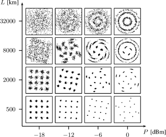
Figure 1: Scatter plots of $Y$ assuming $X\in\mathcal{X}_{\text{16-QAM}}$ for several combinations of transmit power ${P}$ and fiber length ${L}$.

It can be observed that for very low input power and fiber length, nonlinearities are negligible and the channel behaves as a standard AWGN channel. The scatter plots along a diagonal in Fig. 1 correspond to a constant signal-to-(additive-)noise ratio (SNR), defined as $\text{SNR}\triangleq{{P}}/{\sigma^{2}}$. In contrast to an AWGN channel for which the scatter plots along any diagonal would look similar, the received constellation points in Fig. 1 start to rotate in a deterministic fashion and the effect of the NLPN becomes pronounced for large ${L}$ and ${P}$. Therefore, in order to specify the operating point of the channel, the SNR alone is not sufficient, because the parameter space of the channel is two-dimensional, cf. [17, Sec. VII]. In this paper, we present performance results assuming a fixed fiber length and variable transmit power.

II-B Amplitude-Phase Shift Keying

We use the term APSK for the discrete-input constellations considered in this paper and focus on constellations with $M=4$, $8$, and $16$ points. The APSK signal set is defined as [9]

$$\mathcal{X}\triangleq\left\{r_{k}e^{\jmath\left(\frac{2\pi j}{l_{k}}+\varphi_{k}\right)}\;:\;1\leq k\leq N,\quad 0\leq j\leq l_{k}-1\right\},$$ (3)

where $N$ denotes the number of amplitude levels or rings, $r_{k}$ the radius of the $k$th ring, $l_{k}\geq 1$ the number of points in the $k$th ring, where $\sum_{k=1}^{N}l_{k}=M$, and $\varphi_{k}$ the phase offset in the $k$th ring. Throughout the paper, we assume a uniform distribution on the channel input $X$ over all symbols, and thus ${P}=(1/M)\sum_{k=1}^{N}l_{k}r_{k}^{2}$. The radii are assumed to be ordered such that $r_{1}<\ldots<r_{N}$ and we use $\boldsymbol{r}\triangleq(r_{1},\ldots,r_{N})$ to denote the radius vector. In this paper, for $l_{1}=1$, the point in the first ring is always placed at the origin, implying $r_{1}=0$. The radius vector is said to be uniform if $r_{k+1}-r_{k}=\Delta$ for $1\leq k\leq N-1$, where $\Delta=r_{2}$ if $l_{1}=1$ and $\Delta=r_{1}$ if $l_{1}\geq 2$. The symbols are assumed to be indexed, i.e., $x_{i}\in\mathcal{X}$, $i=1,\ldots,M$. The indexing is done starting in the innermost ring ($k=1$) by increasing $j$ from $0$ to $l_{1}-1$ and then moving to the next ring increasing $j$ from $0$ to $l_{2}-1$ and so on. Thus, finally we have $x_{1}=r_{1}e^{\jmath\varphi_{1}},\ldots,x_{M}=r_{N}e^{\jmath 2\pi(l_{N-1})/l_{N}+\varphi_{N}}$.

We also define the vectors $\boldsymbol{l}\triangleq(l_{1},\ldots,l_{N})$ and $\boldsymbol{\varphi}\triangleq(\varphi_{1},\ldots,\varphi_{N})$, and use the notation $\boldsymbol{l}$-APSK for an APSK constellation with $N$ rings and $l_{k}$ points in the $k$th ring, e.g., (4,4,4,4)-APSK. Note that this notation does not specify a particular constellation without ambiguity, due to the missing information about the radii and phase offsets.

III Detection Methods

III-A Symbol Error Probability

Let $\mathcal{R}_{i}$, $1\leq i\leq M$, be the decision region implemented by a detector for the symbol $x_{i}$, i.e., $\hat{X}=x_{i}$ if $Y\in\mathcal{R}_{i}$, where $\hat{X}$ denotes the detected symbol. The average SEP is then

$$\text{SEP}=1-\frac{1}{M}\sum_{i=1}^{M}P_{i\to i},$$ (4)

where $P_{i\to j}\triangleq\text{Pr}[\hat{X}=x_{j}|X=x_{i}]$, $1\leq i,j\leq M$, are the symbol transition probabilities calculated as

$$P_{i\to j}=\int_{\mathcal{R}_{j}}f_{Y|X=x_{i}}(y)\,\mathrm{d}y.$$ (5)

That is, $P_{i\to j}$ is obtained through integration of the conditional PDF of the observation given the channel input $X=x_{i}$ over the detector region for $x_{j}$.

III-B Maximum Likelihood Detection

Let the polar representation of the channel input and the observation be given by $X=R_{0}e^{j\Theta_{0}}$ and $Y=Re^{j\Theta}$, respectively. The PDF of $Y$ can be written in the form [17, Sec. III], [3, p. 225], [28]

$$f_{Y|X=x}(y)=\frac{f_{R|R_{0}=r_{0}}(r)}{2\pi r}+\frac{1}{\pi r}\sum_{m=1}^{\infty}\Re\left\{C_{m}(r,r_{0})e^{\jmath m(\theta-\theta_{0})}\right\},$$ (6)

where $x=r_{0}e^{\jmath\theta_{0}}$, $y=re^{\jmath\theta}$, $\Re\{z\}$ is the real part of $z\in\mathbb{C}$, and the PDF of the received amplitude $R$ given the transmitted amplitude $R_{0}=r_{0}$ is

$$f_{R|R_{0}=r_{0}}(r)=\frac{2r}{\sigma^{2}}\exp\left(-\frac{r^{2}+r_{0}^{2}}{\sigma^{2}}\right){\operatorname{I}_{0}\left(\frac{2rr_{0}}{\sigma^{2}}\right)},$$ (7)

where ${\operatorname{I}_{0}\left(\cdot\right)}$ is the modified Bessel function of the first kind. Analytical expressions for the coefficients $C_{m}(r,r_{0})$ can be found in [17, Sec. III]. The ML detector can now be described in the form of decision regions $\mathcal{R}^{\text{ML}}_{i}\subset\mathbb{C}$ for each symbol $x_{i}\in\mathcal{X}$:

$$\mathcal{R}^{\text{ML}}_{i}\triangleq\bigcap_{\begin{subarray}{c}j=1\\ j\neq i\end{subarray}}^{M}\{y\in\mathbb{C}\;:\;f_{Y|X=x_{i}}(y)\geq f_{Y|X=x_{j}}(y)\}.$$ (8)

If we take the ML decision regions defined in (8), then (4) becomes a lower bound on the achievable SEP with suboptimal detectors.

Evaluating the SEP by numerically integrating over the PDF (6) is computationally expensive. Moreover, unlike for an AWGN channel, where the ML regions simply scale proportionally to $\sqrt{{P}}$, the ML decision regions defined in (8) change their shape based on the transmit power ${P}$ [28]. This renders ML detection rather impractical for the purpose of constellation optimization.

III-C Two-Stage Detection

In this paper, we study a slightly modified version of the suboptimal TS detector proposed in [28]. This detector is a practical alternative to the ML detector because it has much lower complexity. In particular, the TS detector employs one-dimensional decisions: First in the amplitude direction (first detection stage), followed by a phase rotation, and then in the phase direction (second detection stage).

Figure 2: Block diagram of the TS detector. Note that the depicted postcompensation of $Y$ to $\tilde{Y}$ is reversible.

In Fig. 2, we show a block diagram of the TS detector. We refer to the first detection stage together with the phase rotation as postcompensation. Based on the absolute value of the observation $R$, radius detection is performed. In contrast to [28] and [29], we use maximum a posteriori (MAP) instead of ML radius detection and make use of the a priori probability for selecting a certain ring at the transmitter, thereby achieving a small performance advantage. The radius detector implements the rule: Choose $\hat{R}_{0}=r_{k}$, when $\mu_{k-1}\leq R<\mu_{k}$, where $\mu_{k}$, $0\leq k\leq N$, denote the decision radii or thresholds. The MAP decision threshold $\mu_{k}$, $1\leq k\leq N-1$, between $r_{k}$ and $r_{k+1}$ is obtained by solving

$$\operatorname{Pr}\left[{R_{0}=r_{k}}\right]f_{R|R_{0}=r_{k}}(\mu_{k})=\operatorname{Pr}\left[{R_{0}=r_{k+1}}\right]f_{R|R_{0}=r_{k+1}}(\mu_{k}),$$ (9)

where the a priori probabilities are given by $\operatorname{Pr}\left[{R_{0}=r_{k}}\right]=l_{k}/M$. We always define $\mu_{0}\triangleq 0$ and $\mu_{N}\triangleq\infty$. Based on the radius $\hat{R}_{0}$ of the detected ring and the received amplitude $R$, a correction angle $\theta_{c}$ is calculated, by which the observation $Y$ is rotated to obtain the postcompensated observation $\tilde{Y}$ as shown in Fig. 2. The correction angle is given by

$$\theta_{c}(R,\hat{R}_{0})=-\angle C_{1}(R,\hat{R}_{0}),$$ (10)

which is approximately a quadratic function in $R$ [28].

The second detection stage is then performed with respect to $\tilde{Y}$: A phase detector chooses the constellation point with radius $\hat{R}_{0}$ that is closest to $\tilde{Y}$. Graphically, the TS detector employs so called annular sector regions (or annular wedges) as decision regions for $\tilde{Y}$.

III-D PDF of the Postcompensated Observation

It is shown in [28] that for PSK signal sets (which, in this paper, are denoted by $(M)$-APSK) where $\hat{R}_{0}=\sqrt{{P}}=\text{const.}$, a minimum-distance detector for $\tilde{Y}$ is equivalent to ML detection. In contrast, for constellations with multiple amplitude levels, the receiver structure in Fig. 2 does not perform ML detection. However, in principle, optimal detection of $X$ is still possible based on $\tilde{Y}$ due to the fact that the postcompensation in Fig. 2 is invertible and every invertible function forms a sufficient statistic for detecting $X$ based on $Y$ [38, p. 443]. Thus, the performance loss associated with the TS detection scheme originates solely from suboptimal detection regions, not from the postcompensation itself, which is a lossless operation.

In the following, we show how the PDF of the postcompensated observation $\tilde{Y}$ can be computed. This PDF can then be used to find optimal detection regions for $\tilde{Y}$. It is clear from the block diagram of Fig. 2 that the PDF can be written as

$$f_{\tilde{Y}|X=x}(\tilde{y})=f_{Y|X=x}\left(\tilde{y}\cdot e^{-\jmath\theta_{c}(R,\hat{R}_{0})}\right).$$ (11)

Most importantly, the correction angle $\theta_{c}$ is a discontinuous function of the amplitude $R$ because it depends on the detected ring $\hat{R}_{0}$. In general, the correction angle can be written as

$$\theta_{c}(R,\hat{R}_{0})=\begin{cases}\theta_{c}(R,r_{1})\quad\text{if }\mu_{0}\leq R<\mu_{1}\\ \qquad\vdots\qquad\qquad\qquad\vdots\\ \theta_{c}(R,r_{N})\quad\text{if }\mu_{N-1}\leq R<\mu_{N}\\ \end{cases}.$$ (12)

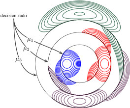
Figure 3: PDF of $\tilde{Y}$ for ${P}=-$5\text{\,}\mathrm{dB}\text{\,}\mathrm{m}$$ and ${L}=$5500\text{\,}\mathrm{km}$$ conditioned on one particular point in each ring of the uniform (4,4,4,4)-APSK constellation. Color is helpful.

For illustration purposes, we plot in Fig. 3 the PDF resulting from (11) and (12) conditioned on one particular point in each ring of the uniform $(4,4,4,4)$-APSK constellation. If we consider the PDF conditioned on $X=r_{2}$, i.e., $R_{0}=r_{2}$ and $\Theta_{0}=0$ (shown in red), it can be observed that the contour lines look as though they have been sliced up along the decision radii of the radius detector. For $R<\mu_{1}$, the correction angle is calculated with respect to $r_{1}$, and thus, the phase is undercompensated. On the other hand, for $R\geq\mu_{2}$, the wrongly detected radius results in an overcompensation.

III-E Performance Comparison

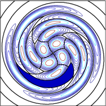
(a) ML decision regions w.r.t. $Y$

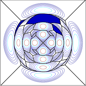
(b) ML decision regions w.r.t. $\tilde{Y}$

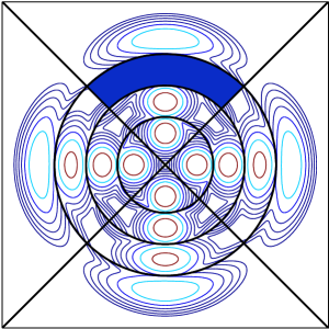
(c) TS decision regions

Figure 4: Decision regions for the uniform $(4,4,4,4)$-APSK constellation at ${P}=$-4\text{\,}\mathrm{dB}\text{\,}\mathrm{m}$$. Shaded regions correspond to the point $X=r_{3}e^{\jmath\pi/2}$.

For a qualitative performance comparison between the different detectors, in Fig. 4LABEL:sub@fig:regions1, the PDF in (6) is plotted for the uniform $(4,4,4,4)$-APSK constellation together with the ML decision regions. In Fig. 4LABEL:sub@fig:regions2, the PDF in (11) is used instead. Finally, Fig. 4LABEL:sub@fig:regions3 shows the same PDF as Fig. 4LABEL:sub@fig:regions2 together with the suboptimal decision regions implemented by the TS detector. As an example, the decision regions corresponding to the point $X=r_{3}e^{\jmath\pi/2}$ are shaded in Fig. 4.

Comparing the optimal decision regions in Fig. 4LABEL:sub@fig:regions2 with the decision regions in Fig. 4LABEL:sub@fig:regions3, it can be seen that TS detection is clearly suboptimal for this constellation and input power. However, one would expect the two small shaded regions in Fig. 4LABEL:sub@fig:regions2 to become smaller for higher power. Intuitively, this is explained by the increasing accuracy of the radius detector for increasing transmit power, due to the Rice distribution (7) of the amplitude. More precisely, let $P^{(e)}_{k}\triangleq\text{Pr}[\hat{R}_{0}\neq R_{0}|R_{0}=r_{k}]$ be the probability of an error in the first detection stage, given that a symbol in the $k$th ring is transmitted. Then

$$P^{(e)}_{k}=1-\left(Q_{\text{1}}\left(\tilde{r}_{k},\tilde{\mu}_{k-1}\right)-Q_{\text{1}}\left(\tilde{r}_{k},\tilde{\mu}_{k}\right)\right),$$ (13)

where $Q_{\text{1}}\left(\cdot,\cdot\right)$ is the Marcum Q-function, $\tilde{r}_{k}\triangleq\sqrt{2}r_{k}/\sigma$, and $\tilde{\mu}_{k}\triangleq\sqrt{2}\mu_{k}/\sigma$. It follows that the SEP under TS detection converges to the SEP under ML detection for increasing input power and any APSK constellation with uniform radius vector, since then $P^{(e)}_{k}$, $1\leq k\leq N$, tends to zero as ${P}$ increases.

IV Constellation Optimization

IV-A Problem Statement

In this section, we optimize the parameters of APSK constellations by minimizing the SEP under TS detection. Formally, the optimization problem can be stated as: Given $M$, ${P}$, and ${L}$,

$$\underset{\boldsymbol{l},\boldsymbol{r}}{\text{minimize}}\qquad$$ SEP under TS detection (14)

subject to $$1\leq N\leq M$$ (15)

$$l_{1}+\ldots+l_{N}=M$$ (16)

$$l_{1}r^{2}_{1}+\ldots+l_{N}r^{2}_{N}=PM$$ (17)

$$l_{k}\geq 1,\text{for }1\leq k\leq N.$$ (18)

The objective function can be computed analytically using (4) with the PDF (11) integrated over the TS detector regions [34, Eq. (4)]. Note that the phase offset vector $\boldsymbol{\varphi}$ does not appear in the minimization problem. This is due to the fact that the SEP under TS detection does not change assuming a phase offset in any of the constellation rings: The PDF of $\tilde{Y}$ is simply rotated by the phase offset, but so is the detector region itself, and hence the integrals in (5) are not affected.

It is instructive to begin by discussing two special cases of the general optimization problem above. The first case is obtained when $\boldsymbol{r}$ is assumed to be uniform and an optimization is performed only over the number of points in each ring $\boldsymbol{l}$, cf. (14)$-$(18). The optimization problem then becomes an integer program which can be solved in an exhaustive fashion for the constellation sizes considered in this paper. The number of ways to distribute $M$ constellation points to $i$ rings is given by ${M-1\choose i-1}$. At most, there are $M$ rings, which gives a total of $\sum_{i=1}^{M}{M-1\choose i-1}=2^{M-1}$ possibilities to choose $\boldsymbol{l}$. There are $8$, $128$, and $32768$ possibilities for $4$, $8$, and $16$ points, respectively. It is clear that such a brute-force approach becomes unfeasible for larger constellations. However, based on the obtained results, it might be possible to devise more sophisticated search methods for $M>16$, e.g., by neglecting unrealistic combinations a priori.

The second special case is given by the optimization of the radius vector $\boldsymbol{r}$ for a certain constellation with fixed parameter $\boldsymbol{l}$. For this case, the optimization problem becomes a nonlinear program. Due to the power constraint, the dimensionality of the search space is $N-1$ if $l_{1}>1$ and $N-2$ if $l_{1}=1$, respectively. By inspecting the target function, one can verify that this problem is nonconvex, i.e., a local optimum does not necessarily imply a global solution. We tested different nonlinear solvers and obtained very good solutions with the Nelder–Mead simplex method [39]. Even though the solution is not guaranteed to be the globally optimal, we verified the global optimality for several constellations and several combinations of input power and fiber length with a brute-force grid search.

By combining the solutions to the two special cases above, a solution to the general optimization problem can then be found as follows: For each APSK constellation with a certain fixed parameter $\boldsymbol{l}$ one determines the optimal radius vector via the simplex method for a given input power and fiber length, and then optimizes over all possible $\boldsymbol{l}$. We call this approach joint optimization.

IV-B Results and Discussion

IV-B1 4 Points

We start by finding optimal APSK constellations with $M=4$ points. The fiber length is fixed at $L=$7000\text{\,}\mathrm{km}$$ and the input power ${P}$ is varied from $-15\text{\,}\mathrm{dB}\text{\,}\mathrm{m}$ to $5\text{\,}\mathrm{dB}\text{\,}\mathrm{m}$ in steps of $0.5\text{\,}\mathrm{dB}\text{\,}\mathrm{m}$. In Fig. 5 we plot the performance of all possible eight 4-point APSK constellations with optimal radius vector (dashed lines) and the curves are labeled with the corresponding $\boldsymbol{l}$. (For $(4)$-APSK and $(1,3)$-APSK the radius vector is fixed, i.e., no optimization is performed.) The results of the joint optimization are shown with markers. We also show the SEP of (4)-APSK (or 4-QAM) in an AWGN channel under ML detection as a well-known reference curve (dash-dotted line). Note that for each ${P}$ the SEP is minimized by a constellation with certain parameters $\boldsymbol{l}$ and $\boldsymbol{r}$. For example, it can be seen that for an input power range between $-15\text{\,}\mathrm{dB}\text{\,}\mathrm{m}$ and $-7.5\text{\,}\mathrm{dB}\text{\,}\mathrm{m}$, $(4)$-APSK is optimal.

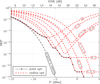
Figure 5: Results for the constellation optimization with $M=4$. The fiber length is $L=$7000\text{\,}\mathrm{km}$$. The dash-dotted line is a reference curve, showing the SEP of $4$-QAM in an AWGN channel under ML detection.

Based on the behavior of the SEP for the individual APSK constellations with optimized radius vector (dashed lines in Fig. 5), it is possible to classify the constellations into three classes. The first class exhibits a well known performance minimum, i.e., an optimal operating power. The second class does not exhibit a minimum, but eventually flattens for very high input power (see, e.g., the performance of $(3,1)$-APSK). The third class exhibits a performance behavior which is strictly and steadily decreasing with increasing input power.

The flattening of the SEP for the second class is explained by the availability of a sacrificial point in the outer constellation ring. The meaning of the term sacrifical is best explained with the help of an example. In Fig. 6 we show the results of the radius optimization for $(3,1)$-APSK (top), together with the optimal values of the parameter $\boldsymbol{r}$ (bottom).

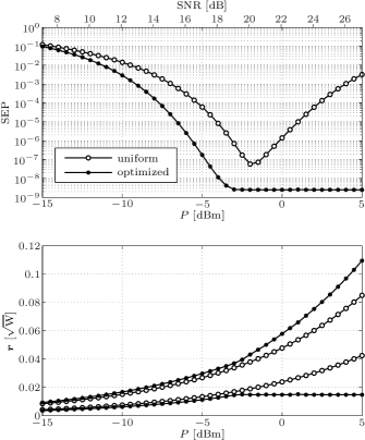
Figure 6: Performance of the $(3,1)$-APSK constellation with a uniform and optimized radius vector (top) and the corresponding radius vector (bottom).

It can be observed that, for ${P}>$-3\text{\,}\mathrm{dB}\text{\,}\mathrm{m}$$, the optimal ring spacing shows a very peculiar behavior. For this power regime, $r_{1}$ appears to be fixed and any increase in average power is absorbed by putting the outermost point further away from the inner ring. In some sense, the outer point (experiencing very high NLPN) is sacrificed with the result of saving the average SEP of the constellation. Observe that $(1,1,1,1)$-APSK is the only APSK constellation with 4 points that belongs to the third class and it was already argued in [28], that this constellation is optimal for very high input power.

The system parameters are chosen in such a way that the obtained results are directly comparable to the performance of the optimized constellations presented in [28, Sec. IV]. To facilitate a comparison, in Fig. 7 we provide a digitalized version of [28, Fig. 15] and plot the outcome of the joint optimization in the same figure. All four constellations used in [28] can be seen as APSK constellations and they are depicted in Fig. 7 for convenience. With the notation introduced in this paper, the constellations are $(4)$-APSK, $(1,3)$-APSK, $(2,2)$-APSK with $\boldsymbol{\varphi}=(0,\varphi_{2})$, and $(1,2,1)$-APSK with $\boldsymbol{\varphi}=(0,0,\varphi_{3})$. The parameters $\varphi_{2}$ and $\varphi_{3}$ are determined by a precompensation technique developed in [28], while the radius vector of the two latter constellations was optimized.

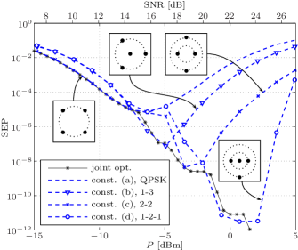
Figure 7: Comparison between the joint optimization of the 4-point APSK constellation and the results for optimized constellations (a)–(d) in [28] under ML detection. The legend shows the constellation names originally used in [28].

It is important to point out that the optimization in [28] was performed with respect to ML detection, while for the joint optimization in this paper the suboptimal TS detector is assumed. Notice that, for $(4)$-APSK these two detection schemes are equivalent and hence, the performance results taken from [28] for $(4)$-APSK (constellation $(a)$) in Fig. 7 overlap with the results of the joint optimization for an input power up to $-7.5\text{\,}\mathrm{dB}\text{\,}\mathrm{m}$. Comparing the results in Fig. 7, it can be seen that the jointly optimized APSK constellations perform very close to the optimized constellations in [28]. For certain input powers, e.g., $-7\text{\,}\mathrm{dB}\text{\,}\mathrm{m}$ or $-5\text{\,}\mathrm{dB}\text{\,}\mathrm{m}$, a performance loss is visible, which is explained by the weaker detection technique. On the other hand, for some power regimes, e.g., $-3.5\text{\,}\mathrm{dB}\text{\,}\mathrm{m}$ or $-2\text{\,}\mathrm{dB}\text{\,}\mathrm{m}$, the jointly optimized constellations perform as well as, or even outperform, the best constellations presented in [28]. We attribute this performance gain to the more systematic search which is offered by the APSK framework. Also note that there is no need to find phase precompensation angles as was done in [28], because those are relevant only for ML detection, but irrelevant for the performance under TS detection. This removes one degree of freedom from choosing a constellation and makes the optimization simpler. As a last point, it is unclear why constellation (d) in [28] does not exhibit a flattening SEP for very high input power, even though the radius vector was optimized and a sacrificial point is available. We conjecture that the SEP results for constellation (d) for $3\text{\,}\mathrm{dB}\text{\,}\mathrm{m}$ and $5\text{\,}\mathrm{dB}\text{\,}\mathrm{m}$ are only locally optimal.

IV-B2 8 Points

For $M=8$ points, we present optimization results for the same system parameters as before. The results for the joint optimization are shown in Fig. 8 with markers.

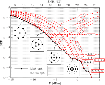
Figure 8: Results for the constellation optimization with $M=8$. The fiber length is $L=$7000\text{\,}\mathrm{km}$$.

Since it is not very instructive to show the performance of all 8-point APSK constellations in the same figure, we only plot the SEP of those constellations that are optimal somewhere in the considered power range (dashed lines). Thus, the parameter $\boldsymbol{l}$ is indicated by the labeling of the corresponding dashed line. To avoid cumbersome notation, we also define $\boldsymbol{1}_{N}\triangleq 1,\ldots,1$ ($N$ times). To get a more intuitive feeling for the optimal constellations in different power regimes, the inset figures show the actual constellations that are optimal at $-12\text{\,}\mathrm{dB}\text{\,}\mathrm{m}$, $-7.5\text{\,}\mathrm{dB}\text{\,}\mathrm{m}$, $-4.5\text{\,}\mathrm{dB}\text{\,}\mathrm{m}$, and $-1\text{\,}\mathrm{dB}\text{\,}\mathrm{m}$. The constellations are shown with their optimized radius vector for the corresponding input power.

We also perform an optimization only over $\boldsymbol{l}$ assuming that the radius vector is uniform. The results are depicted in Fig. 9. To facilitate a better comparison with the jointly optimized constellations, the solid black line in Fig. 8 is again plotted in Fig. 9. The dashed lines in Fig. 9 show the SEP of the APSK constellation with a fixed parameter $\boldsymbol{l}$ and assuming a uniform radius vector. An important observation here is that up to an input power of $-3.5\text{\,}\mathrm{dB}\text{\,}\mathrm{m}$, there is almost no difference between the performance of the jointly optimized constellations and the optimal constellations obtained assuming a uniform radius vector, suggesting that most of the performance improvement is due to optimizing the parameter $\boldsymbol{l}$.

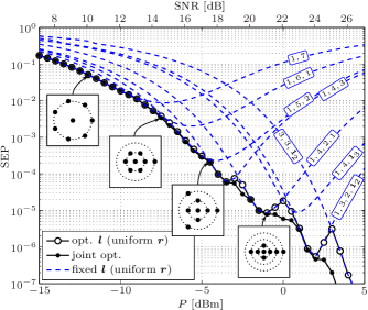
Figure 9: Results for the constellation optimization with $M=8$ (white circles) assuming that a uniform radius vector for all constellations. The fiber length is $L=$7000\text{\,}\mathrm{km}$$. The results of the joint optimization from Fig. 8 (black markers) are shown for comparison. The dashed lines correspond to the SEP of the constellations that are indicated by the labels.

IV-B3 16 Points

Motivated by the results obtained for $M=8$, for $M=16$ points, we limit ourselves to the case where the radius vector is assumed to be uniform for all constellations. The fiber length is ${L}=$5500\text{\,}\mathrm{km}$$ and the input power ${P}$ is varied from $-14\text{\,}\mathrm{dB}\text{\,}\mathrm{m}$ to $10\text{\,}\mathrm{dB}\text{\,}\mathrm{m}$ in steps of $2\text{\,}\mathrm{dB}\text{\,}\mathrm{m}$. The results are shown in Fig. 10, where we indicate the optimal parameter $\boldsymbol{l}$ next to the corresponding marker of the curve.

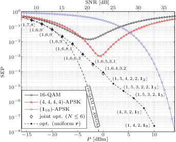
Figure 10: Results for the constellation optimization with $M=16$. The SEP under TS detection for 16-QAM, uniform $(4,4,4,4)$-APSK, and $(\boldsymbol{1}_{16})$-APSK are shown for comparison. The SEP under ML detection for 16-QAM in an AWGN channel (dash-dotted line) is shown as a reference.

The individual SEP under TS detection for 16-QAM, uniform $(4,4,4,4)$-APSK, and $(\boldsymbol{1}_{16})$-APSK are shown for comparison, while the SEP under ML detection for 16-QAM in an AWGN channel is shown as a reference. The results in Fig. 10 show that up to an input power of $-8\text{\,}\mathrm{dB}\text{\,}\mathrm{m}$, the performance of the optimized constellations follows closely the performance of 16-QAM in AWGN. In other words, for this power regime it is possible to find APSK constellations with TS detection that perform as well as 16-QAM for a channel without nonlinear impairments under ML detection. For higher input power, the optimized constellations gradually utilize more amplitude levels, due to the increase in NLPN. If we take as a baseline the minimum SEP achieved by the 16-QAM constellation (${P}\approx$-2.8\text{\,}\mathrm{dB}\text{\,}\mathrm{m}$$ and SEP $\approx 10^{-2}$), and interpolate the optimal APSK performance for the same SEP, we observe that a performance gain of $3.2\text{\,}\mathrm{dB}\text{\,}\mathrm{m}$ is achieved.

In order to verify the assumption that a joint optimization approach does not lead to significant performance gains, we also perform a reduced complexity approach to the joint optimization, where the optimization is restricted to constellations with at most $N=6$ rings. This makes the results meaningful only for low and moderate input power ($P\leq$0\text{\,}\mathrm{dB}\text{\,}\mathrm{m}$$), because, as we have seen previously, for higher input power, the dominance of the NLPN dictates the use of more amplitude levels to achieve good performance. The results are also shown in Fig. 10 for ${P}\leq$0\text{\,}\mathrm{dB}\text{\,}\mathrm{m}$$ (diamond markers). It can be seen that the jointly optimized constellations with the additional constraint $N\leq 6$ follow closely the performance of the constellations obtained for a uniform radius vector, confirming that the joint optimization only yields negligible performance improvements for this power regime. For higher input power, the obtained jointly optimized constellations perform worse than the optimal constellations obtained with a uniform radius vector, which is simply due to the restriction to six rings.

Finally, the phenomenon of sacrificial points discussed previously also generalizes to entire rings, i.e., when optimizing the radius vector of constellations with more than one point in the outer ring. In this case, however, the SEP still exhibits a minimum. As an example, in Fig. 11 we show the result of the radius optimization for $(4,4,4,4)$-APSK (top) together with the optimal radius vector (bottom). The radius vector $\boldsymbol{r}$ is plotted in a normalized fashion $\boldsymbol{\tilde{r}}=\boldsymbol{r}/\sqrt{{P}}$ (i.e., $\sum_{i=1}^{N}l_{i}\tilde{r}_{i}^{2}=1$), so that the effect is more clear. It can be observed that up to an input power of $4\text{\,}\mathrm{dB}\text{\,}\mathrm{m}$ the distance between any two adjacent rings for the optimal radius vector is approximately the same. Moreover the distance decreases with higher input power (like “squeezing accordion pleats” [31]). However, for $P>$4\text{\,}\mathrm{dB}\text{\,}\mathrm{m}$$ the optimal radius vector changes significantly. Somewhat counterintuitively, in this power regime, is is better to place the four points in the outer constellation ring far away from the other rings.

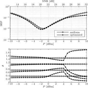
Figure 11: Illustration of a sacrificial ring which occurs for the radius optimization of $(4,4,4,4)$-APSK for ${P}>$4\text{\,}\mathrm{dB}\text{\,}\mathrm{m}$$. The system length is ${L}=$7000\text{\,}\mathrm{km}$$.

V Binary Labelings

In order to allow for the transmission of binary data, we assume that each symbol $x_{i}\in\mathcal{X}$ is labeled with a binary vector $\boldsymbol{c}_{i}=(c_{i,1},\ldots,c_{i,m})\in\{0,1\}^{m}$, where $m=\log_{2}M$. The different binary vectors are the binary representations of the integers $\{0,1,\dots,M-1\}$. A specific mapping between vectors and constellation symbols is called a binary labeling, which will be denoted by an $M\times m$ matrix $\mathbb{L}_{m}=(\boldsymbol{c}_{1}^{T},\ldots,\boldsymbol{c}_{M}^{T})^{T}$.

A Gray labeling is obtained if the binary vectors of neighboring symbols, i.e., symbols that are closest in terms of Euclidean distance, differ by only one bit position. As an example, the Gray labeling $\mathbb{G}_{m}$ for $(M)$-APSK constellations may be constructed by $m-1$ recursive reflections of the trivial labeling $\mathbb{G}_{1}=(0,1)^{T}$. To obtain $\mathbb{G}_{m+1}$ from $\mathbb{G}_{m}$ by reflection, generate the matrix $(\boldsymbol{c}_{1}^{T},\ldots,\boldsymbol{c}_{M}^{T},\boldsymbol{c}_{M}^{T},\ldots,\boldsymbol{c}_{1}^{T})^{T}$ and add an extra column from the left, consisting of $M$ zeros followed by $M$ ones [40].

V-A Bit Error Probability

The average BEP of the signal constellation is given by

$$\text{BEP}=\frac{1}{mM}\sum_{i=1}^{M}\sum_{j=1\atop j\neq i}^{M}d_{\text{H}}(\boldsymbol{c}_{i},\boldsymbol{c}_{j})\cdot P_{i\to j},$$ (19)

where $d_{\text{H}}(\cdot,\cdot)$ denotes the Hamming distance between two binary vectors. A lower bound for the BEP is $\text{SEP}/m\leq\text{BEP}$, which directly follows from $1\leq d_{\text{H}}(\boldsymbol{c}_{i},\boldsymbol{c}_{j})$, $i\neq j$.

The probabilities $P_{i\to j}$ are fixed for a given constellation and ${P}$ and ${L}$ (cf. (5)), hence (19) depends only on the labeling. However, it is important to realize that the phase offset vector $\boldsymbol{\varphi}$ has an effect on these probabilities for $j\neq i$. Therefore, even though two APSK constellations with the same $\boldsymbol{l}$ and $\boldsymbol{r}$ but different $\boldsymbol{\varphi}$ have the same SEP, they may have a different BEP. In the following, we show how to exploit this new degree of freedom for a class of APSK constellations that permit the use of a Gray labeling.

V-B Rectangular APSK

APSK constellations with $1<N<M$, $\boldsymbol{\varphi}=\boldsymbol{0}$ and $l\triangleq l_{k}=M/N$, $1\leq k\leq N$, have a “rectangular” structure when plotted in polar coordinates. For these constellations, a Gray labeling is given by $\mathbb{L}_{m}=\mathbb{G}_{\log_{2}N}\otimes\,\mathbb{G}_{\log_{2}l}$, where $\otimes$ is the ordered direct product, defined as

$$(\boldsymbol{a}_{1}^{T},\ldots,\boldsymbol{a}_{p}^{T})^{T}\otimes(\boldsymbol{b}_{1}^{T},\ldots,\boldsymbol{b}_{q}^{T})^{T}=(\boldsymbol{c}_{1}^{T},\ldots,\boldsymbol{c}_{pq}^{T})^{T},$$ (20)

where $\boldsymbol{c}_{qi+j}=(\boldsymbol{a}_{i},\boldsymbol{b}_{j})$, for $1\leq i\leq p$ and $1\leq j\leq q$. This amounts to independently choosing a Gray labeling for the radius and phase coordinates of the constellation and then concatenating the binary vectors. In Fig. 12(b) (top) an example for such a construction is shown.

Gray labelings ensure that for a standard AWGN channel the BEP closely approaches the lower BEP bound for high SNR in Sec. V-A. Using the same labeling in a nonlinear channel, however, does not necessarily ensure good performance since it is constructed without considering the underlying PDF of the observation. From Fig. 3 it is evident that this PDF has a rather unusual shape, due to the slicing effect caused by the postcompensation. To further illustrate this point, consider $(4,4)$-APSK with $r_{1}/r_{2}=0.424$ and $\boldsymbol{\varphi}=(0,0)$, operating at ${L}=$7000\text{\,}\mathrm{km}$$ and ${P}=$-5\text{\,}\mathrm{dB}\text{\,}\mathrm{m}$$, which is the optimal APSK constellation for these parameters (cf. Fig. 8). The PDF of $\tilde{Y}$ conditioned on one point in each ring is evaluated and plotted in polar coordinates, as shown in Fig. 12(a) for $x_{3}$ and $x_{7}$.

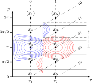
(a) Illustration in polar coordinates

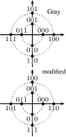
(b) Labeled Const.

Figure 12: In (a), the PDF of $\tilde{Y}$ is shown for $(4,4)$-APSK conditioned on $X=x_{3}$ (blue) and $X=x_{7}$ (red) for ${L}=$7000\text{\,}\mathrm{km}$$ and ${P}=$-5\text{\,}\mathrm{dB}\text{\,}\mathrm{m}$$. Solid lines correspond to the decision boundaries of the TS detector and dotted lines show connections between neighboring symbols according to the PDF.

The solid lines correspond to the decision boundaries of the TS detector. Recalling that the symbol transition probabilities are obtained through integration of the PDF over the detector regions (cf. (5)), Fig. 12(a) can then be used to identify “neighboring symbols” of $x_{3}$ and $x_{7}$ (and consequently of all points) in the sense that the corresponding transition probabilities will dominate in (19). The main observation here is that, even though $x_{3}$ and $x_{7}$ are adjacent symbols in radial direction, the corresponding transition probabilities, i.e., $P_{3\to 7}$ and $P_{7\to 3}$, are negligible compared to $P_{3\to 8}$ and $P_{7\to 2}$, respectively. The dotted lines in Fig. 12(a) show appropriate connections between neighboring symbols taking into account the nonlinear PDF. In Fig. 12(b) the $(4,4)$-constellation is shown with the Gray labeling $\mathbb{G}_{1}\otimes\,\mathbb{G}_{2}$ (top) and the modified labeling (bottom) that results from “following” the dotted lines in Fig. 12(a) and concatenating the binary vectors.

Observe that the labeled constellation in the bottom of Fig. 12(b) may be obtained from the Gray labeled constellation by using a phase offset vector of $\boldsymbol{\varphi}=(0,\pi/2)$: In this case, the non-zero phase offset in the second ring does not change the constellation (i.e., the set of symbols), but rather leads to a different indexing of symbols (cf. Sec. II-B), and consequently to a different mapping between symbols and binary vectors. Going one step further, we now allow for arbitrary phase offsets in all constellation rings, with the intention to “steer” the phase decision boundaries such that they are roughly symmetric around the PDF. Starting from a Gray labeled rectangular APSK constellation, a simple way to achieve this is by initializing $\varphi_{1}=0$ and then calculating

$$\varphi_{i}=\theta_{c}(\mu_{i-1},r_{i-1})-\theta_{c}(\mu_{i-1},r_{i})+\varphi_{i-1},$$ (21)

for $i=2,\ldots,N$. For the previous example, evaluating (21) for $i=2$ results in $\varphi_{2}\approx 1.878$, corresponding to the length of the dashed, grey arrow in 12(a). The two dashed, grey lines are the new phase decision boundaries for $x_{7}$ and it can be seen that they appear roughly symmetric around the blue PDF. We highlight that this proposed method to determine the phase offset vector may be applied to any rectangular APSK constellation of arbitrary constellation size, provided that $M$ is a power of 2.

V-C Results and Discussion

In Fig. 13, the lower bound (LB) for the BEP is plotted for (4,4)-APSK with optimized $\boldsymbol{r}$ and ${L}=$7000\text{\,}\mathrm{km}$$ (black, dashed line). The average BEP of the labeled constellation is shown with the proposed phase offset vector (red markers) and $\boldsymbol{\varphi}=\boldsymbol{0}$, resulting in the conventional Gray labeling (blue, dashed line). The performance with the proposed method is almost indistinguishable from the lower bound and a gain of approximately $0.4\text{\,}\mathrm{dB}$ is visible at $\text{SEP}=10^{-3}$ over the Gray labeling approach.

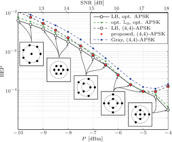
Figure 13: Average BEP and lower bounds (LB) for $M=8$ and ${L}=$7000\text{\,}\mathrm{km}$$ for different APSK constellations. The subfigures show the optimized APSK constellations for the corresponding input power.

Moreover, in Fig. 13 we plot the LB based on the jointly optimized APSK constellations with $M=8$ (cf. Fig. 8), where the subfigures are provided to show the optimal parameter $\boldsymbol{l}$ for the different input powers. For each input power, the optimal labeling is determined exhaustively and the corresponding BEP is shown by the green line. Note that the LB is tight only for the rectangular $(4,4)$-APSK. The results demonstrate that first optimizing the constellation with respect to SEP and then choosing an optimal labeling does not guarantee to give the best BEP performance. In particular, for $-7\text{\,}\mathrm{dB}\text{\,}\mathrm{m}$ and $-6.5\text{\,}\mathrm{dB}\text{\,}\mathrm{m}$, (4,4)-APSK with the proposed phase offset vector achieves a lower BEP than the jointly optimized constellations (with respect to SEP) with an optimal labeling.

As a last point, one might argue that the class of rectangular APSK constellations is not particularly interesting, because they appear rarely as optimal APSK constellations with respect to SEP (e.g., for $M=8$ they only appear in a small power range and for $M=16$ they do not appear at all). However, the previous results show that if we take the BEP as the main figure of merit, rectangular APSK constellations may be advantageous in certain power regimes, because they can closely approach the lower BEP bound. Moreover, as we described earlier, the proposed labeling method is easily applicable to any constellation size. It would therefore be relatively simple to find optimal rectangular APSK constellations for $M>16$ because in this case not many choices exist. Obviously, these constellations might then be far away from the performance of the true optimal constellation, but they might still offer a significant performance gain over rectangular QAM constellations in the presence of NLPN, with the advantage that a constructive labeling method is readily available.

VI Conclusion

In this paper, we optimized APSK constellations for a fiber-optical channel model without dispersion. It was shown how to derive the PDF of the postcompensated observation assuming a TS detection scheme. The PDF was used to gain insight into the performance behavior with respect to optimal detection and to calculate the BEP. Optimal APSK constellations under TS detection have been presented. For $M=16$ constellation points, significant performance improvements in terms of SEP can be achieved by choosing an optimized APSK constellation compared to a baseline 16-QAM constellation. For very high input power, we showed that sacrificing points or constellation rings may become beneficial. Finally, the binary labeling problem was discussed and a constructive labeling method was presented, which is applicable to rectangular APSK constellations. An important topic for future work would be the investigation of the influence of fiber chromatic dispersion and nonlinearities on the optimal signal set.

References

- [1] I. Djordjevic, W. Ryan, and B. Vasic, Coding for Optical Channels. Springer, 2010.
- [2] G. P. Agrawal, Nonlinear Fiber Optics, 4th ed. Academic Press, 2006.
- [3] K.-P. Ho, Phase-modulated Optical Communication Systems. Springer, 2005.
- [4] L. Hanzo, W. Webb, and T. Keller, Single- and Multi-carrier Quadrature Amplitude Modulation: Principles and Applications for Personal Communications, WLANs and Broadcasting. Wiley, 2000.
- [5] G. J. Foschini, R. D. Gitlin, and S. B. Weinstein, “On the selection of a two-dimensional signal constellation in the presence of phase jitter and gaussian noise,” Bell Syst. Tech. J, vol. 52, no. 6, pp. 927–965, Jul. 1973.
- [6] ——, “Optimization of two-dimensional signal constellations in the presence of gaussian noise,” IEEE Trans. Commun., vol. 22, no. 1, pp. 28–38, Jan. 1974.
- [7] C. M. Thomas, M. Y. Weidner, and S. H. Durrani, “Digital amplitude-phase keying with M-ary alphabets,” IEEE Trans. Commun., vol. 22, no. 2, pp. 168–180, Feb. 1974.
- [8] E. Biglieri, “High-level modulation and coding for nonlinear satellite channels,” IEEE Trans. Commun., vol. 32, no. 5, pp. 616–626, May 1984.
- [9] R. De Gaudenzi, A. Guillén i Fàbregas, and A. Martinez, “Performance analysis of turbo-coded apsk modulations over nonlinear satellite channels,” IEEE Trans. Wireless Commun., vol. 5, no. 9, pp. 2396–2407, Sep. 2006.
- [10] W. Sung, S. Kang, P. Kim, D. Chang, and D. Shin, “Performance analysis of APSK modulation for DVB-S2 transmission over nonlinear channels,” Int. J. Commun. Syst. Network, vol. 27, no. 6, pp. 295–311, Nov. 2009.
- [11] European Telecommunications Standards Institute, “Digital video broadcasting (DVB) - second generation framing structure, channel coding and modulation systems for broadcasting, interactive services, news gathering and other broadband satellite applications (DVB-S2),” Sep. 2009. [Online]. Available: http://www.dvb.org/technology/standards/index.xml
- [12] G. P. Agrawal, Fiber-optic Communication Systems, 4th ed. Wiley-Interscience, 2010.
- [13] B. W. Göbel, “Information-theoretic aspects of fiber-optic communication channels,” Ph.D. dissertation, TU Munich, Munich, 2010.
- [14] R.-J. Essiambre, G. Kramer, P. J. Winzer, G. J. Foschini, and B. Göbel, “Capacity limits of optical fiber networks,” J. Lightw. Technol., vol. 28, no. 4, pp. 662–701, Feb. 2010.
- [15] J. P. Gordon and L. F. Mollenauer, “Phase noise in photonic communications systems using linear amplifiers,” Opt. Lett., vol. 15, no. 23, pp. 1351–1353, Dec. 1990.
- [16] A. Mecozzi, “Limits to long-haul coherent transmission set by the kerr nonlinearity and noise of the in-line amplifiers,” J. Lightw. Technol., vol. 12, no. 11, pp. 1993–2000, Nov. 1994.
- [17] M. I. Yousefi and F. R. Kschischang, “On the per-sample capacity of nondispersive optical fibers,” IEEE Trans. Inf. Theory, vol. 57, no. 11, pp. 7522–7541, Nov. 2011.
- [18] K. S. Turitsyn, S. A. Derevyanko, I. V. Yurkevich, and S. K. Turitsyn, “Information capacity of optical fiber channels with zero average dispersion,” Phys. Rev. Lett., vol. 91, no. 20, p. 203901, Nov. 2003.
- [19] E. Ip, “Nonlinear compensation using backpropagation for polarization-multiplexed transmission,” J. Lightw. Technol., vol. 28, no. 6, pp. 939–951, Mar. 2010.
- [20] A. Carena, V. Curri, G. Bosco, P. Poggiolini, and F. Forghieri, “Modeling of the impact of nonlinear propagation effects in uncompensated optical coherent transmission links,” J. Lightw. Technol., vol. 30, no. 10, pp. 1524–1539, May 2012.
- [21] L. Beygi, E. Agrell, P. Johannisson, M. Karlsson, and H. Wymeersch, “A discrete-time model for uncompensated single-channel fiber-optical links,” IEEE Trans. Commun., vol. 60, no. 11, pp. 3440–3450, Nov. 2012.
- [22] A. G. Green, P. P. Mitra, and L. G. L. Wegener, “Effect of chromatic dispersion on nonlinear phase noise,” Opt. Lett., vol. 28, no. 24, pp. 2455–2457, Dec. 2003.
- [23] S. Kumar, “Effect of dispersion on nonlinear phase noise in optical transmission systems,” Opt. Lett., vol. 30, no. 24, pp. 3278–3280, Dec. 2005.
- [24] K.-P. Ho and H.-C. Wang, “Effect of dispersion on nonlinear phase noise.” Opt. Lett., vol. 31, no. 14, pp. 2109–11, Jul. 2006.
- [25] A. Demir, “Nonlinear phase noise in optical-fiber-communication systems,” J. Lightw. Technol., vol. 25, no. 8, pp. 2002–2032, Aug. 2007.
- [26] S. Kumar, “Analysis of nonlinear phase noise in coherent fiber-optic systems based on phase shift keying,” J. Lightw. Technol., vol. 27, no. 21, pp. 4722–4733, Nov. 2009.
- [27] A. Bononi, P. Serena, and N. Rossi, “Nonlinear signal-noise interactions in dispersion-managed links with various modulation formats,” Opt. Fiber. Techn., vol. 16, no. 2, pp. 73–85, Mar. 2010.
- [28] A. P. T. Lau and J. M. Kahn, “Signal design and detection in presence of nonlinear phase noise,” J. Lightw. Technol., vol. 25, no. 10, pp. 3008–3016, Oct. 2007.
- [29] L. Beygi, E. Agrell, and M. Karlsson, “Optimization of 16-point ring constellations in the presence of nonlinear phase noise,” in Proc. Optical Fiber Communication Conf. (OFC), Los Angeles, CA, Mar. 2011.
- [30] N. Ekanayake and H. M. V. R. Herath, “Effect of nonlinear phase noise on the performance of m-ary psk signals in optical fiber links,” J. Lightw. Technol., vol. 31, no. 3, pp. 447–454, Feb. 2013.
- [31] T. Freckmann, R.-J. Essiambre, P. J. Winzer, G. J. Foschini, and G. Kramer, “Fiber capacity limits with optimized ring constellations,” IEEE Photon. Technol. Lett., vol. 21, no. 20, pp. 1496–1498, Oct. 2009.
- [32] J. Zhang and I. B. Djordjevic, “Optimum signal constellation design for rotationally symmetric optical channel with coherent detection,” in Proc. Optical Fiber Communication Conf. (OFC), Beijing, China, Mar. 2011.
- [33] I. B. Djordjevic, T. Liu, L. Xu, and T. Wang, “Optimum signal constellation design for high-speed optical transmission,” in Proc. Optical Fiber Communication Conf. (OFC), Los Angeles, CA, Mar. 2012.
- [34] L. Beygi, E. Agrell, P. Johannisson, and M. Karlsson, “A novel multilevel coded modulation scheme for fiber optical channel with nonlinear phase noise,” in Proc. IEEE Glob. Communication Conf. (GLOBECOM), Miami, FL, Dec. 2010.
- [35] E. Agrell and M. Karlsson, “Satellite constellations: Towards the nonlinear channel capacity,” in Proc. IEEE Photon. Conf., Burlingame, CA, Sep. 2012.
- [36] E. Agrell, “On monotonic capacity–cost functions,” Sep. 2012. [Online]. Available: http://arxiv.org/abs/1209.2820
- [37] G. Caire, G. Taricco, and E. Biglieri, “Bit-interleaved coded modulation,” IEEE Trans. Inf. Theory, vol. 44, no. 3, pp. 927–946, May 1998.
- [38] A. Lapidoth, A Foundation in Digital Communication. Cambridge University Press, 2009.
- [39] J. A. Nelder and R. Mead, “A simplex method for function minimization,” Computer J., vol. 7, no. 4, pp. 308–313, Jul. 1965.
- [40] E. Agrell, J. Lassing, E. Ström, and T. Ottosson, “On the optimality of the binary reflected gray code,” IEEE Trans. Inf. Theory, vol. 50, no. 12, pp. 3170–3182, Dec. 2010.
- [41] Y. Huang and J. Ritcey, “Optimal constellation labeling for iteratively decoded bit-interleaved space-time coded modulation,” IEEE Trans. Inf. Theory, vol. 51, no. 5, pp. 1865–1871, May 2005.