Density functional approaches to nuclear dynamics

Abstract

We present background concepts of the nuclear density functional theory (DFT) and applications of the time-dependent DFT with the Skyrme energy functional for nuclear response functions. Practical methods for numerical applications of the time-dependent Hartree-Fock-Bogoliubov theory (TDHFB) are proposed; finite amplitude method and canonical-basis TDHFB. These approaches are briefly reviewed and some numerical applications are shown to demonstrate their feasibility.

1 Introduction

The nucleus is a quantum object. The nuclear interaction is not strong enough to localize the nucleonic wave function, thus, the nuclear matter stays in the liquid phase even at zero temperature [1]. This strong quantum nature in nuclei leads to a rich variety of unique phenomena. Extensive studies have been made for constructing theoretical models to elucidate basic nuclear dynamics behind a variety of nuclear phenomena. Simultaneously, significant efforts have been made in the microscopic foundation of those models.

Although there have been significant developments in the “first-principles” large-scale computation, starting from the bare nucleon-nucleon (two-body & three-body) forces, they are still limited to light nuclei with small mass numbers, typically $A\lesssim 10$ [2]. In contrast, the density functional theory (DFT) is currently a leading theory for describing nuclear properties of heavy nuclei [3, 4]. It is capable of describing almost all nuclei, including nuclear matter, with a single universal energy density functional (EDF). In addition, its strict theoretical foundation is given by the basic theorem of the DFT [5, 6]. Since the nucleus is a self-bound system without an external potential, the DFT theorem should be modified from its original form. This problem was addressed by recent studies [7, 8, 9]. In this paper, we present basic concepts of the EDF in nuclei and feasible methodologies of the time-dependent DFT.

2 Backgrounds of nuclear energy density functionals

In this section, basic properties of nuclei and historical developments in nuclear structure theory, which leads to the nuclear energy density functional, are briefly reviewed. To simplify the discussion here, we consider an infinite uniform nuclear matter neglecting the Coulomb interaction.

2.1 Basic property of nuclear systems: Saturation and independent-particle motion

2.1.1 Saturation

The volume and total binding energy of observed nuclei in nature are approximately proportional to the mass number $A$. In other words, they have an approximately constant density $\rho_{0}\approx 0.17$ fm^-3 and a constant binding energy per particle $B/A\approx 8$ MeV. Thus, extrapolating this property to the infinite nuclear matter neglecting the Coulomb interaction, the nuclear matter should have an equilibrium state with $\rho_{0}\approx 0.17$ fm^-3 and $B/A\approx 16$ MeV, at zero pressure and zero temperature. This property are called “saturation property”, that is analogous to the liquid. The most famous and successful model based on this liquid picture of nuclei is the empirical mass formula of Bethe and Weizsäcker [10, 11]. This formula contains the surface and Coulomb terms in addition to the leading term proportional to $A$, which well accounts of the bulk part of the nuclear binding.

2.1.2 Independent-particle motion in nuclei

There are many evidences for the fact that the mean-free path of nucleons is larger than the size of nucleus. The great success of the nuclear shell model [12] gives such an example, in which nucleons are assumed to move independently inside an average one-body potential. The scattering experiments with incident neutrons and protons provide more quantified information on the mean-free path. In fact, the mean free path depends on the nucleon’s energy, and becomes larger for lower energy [1]. Therefore, it is natural to assume that the nucleus can be primarily approximated by the independent-particle model with an average one-body potential. For the nuclear matter, this approximation leads to the degenerate Fermi gas of the same number of protons and neutrons ($Z=N=A/2$). The observed saturation density of $\rho_{0}\approx 0.17$ fm^-3 gives the Fermi momentum, $k_{F}\approx 1.36$ fm^-1, which corresponds to the Fermi energy (the maximum kinetic energy), $T_{F}=k_{F}^{2}/2M\approx 40$ MeV.

2.2 Problems of a mean-field picture

Evidences of the independent-particle motion encourage us to adopt the mean-field picture of nuclei. However, it turned out that the mean-field models cannot describe the nuclear saturation property. Let us explain this for the uniform nuclear matter with a constant attractive potential $V<0$.

The constancy of $B/A$ means that it is equal to the separation energy of nucleons, $S$. In the Fermi-gas model, it is estimated as

$$S\approx B/A\approx-(T_{F}+V).$$ (1)

Since the binding energy is $B/A\approx 16$ MeV, the potential $V$ is about $-55$ MeV. It should be noted that the relatively small separation energy is the consequence of the significant cancellation between kinetic and potential energies. In the mean-field theory, the total (binding) energy is given by

$$-B=\sum_{i=1}^{A}\left(T_{i}+\frac{V}{2}\right)=A\left(\frac{3}{5}T_{F}+\frac{V}{2}\right),$$ (2)

where we assume that the average potential results from a two-body interaction. The two kinds of expressions for $B/A$, Eqs. (1) and (2), lead to $T_{F}\approx-5V/4\approx 70$ MeV, which is different from the previously estimated value ($\sim 40$ MeV). Moreover, the negative separation energy ($T_{F}+V>0$) contradicts the fact that the nucleus is bound!

To reconcile the independent-particle motion with the saturation property of the nucleus, the nuclear average potential must be state dependent. Allowing the potential $V_{i}$ depend on the state $i$, the potential $V$ should be replaced by that for the highest occupied orbital $V_{F}$ in Eq. (1), and by its average value $\langle V\rangle$ in the right-hand side of Eq. (2). Then, we obtain the following relation:

$$V_{F}\approx\langle V\rangle+T_{F}/5+B/A.$$ (3)

Therefore, the potential $V_{F}$ is shallower than its average value.

Weisskopf suggested the momentum-dependent potential $V$, which can be expressed in terms of an effective mass $m^{*}$ [13]:

$$V_{i}=U_{0}+U_{1}\frac{k_{i}^{2}}{k_{F}^{2}}.$$ (4)

Actually, if the mean-field potential is non-local, it can be expressed by the momentum dependence. Equation (4) leads to the effective mass, $m^{*}/m=(1+U_{1}/T_{F})^{-1}$. Using Eqs. (1), (3), and (4), we obtain the effective mass given by

$$\frac{m^{*}}{m}=\left\{\frac{3}{2}+\frac{5}{2}\frac{B}{A}\frac{1}{T_{F}}\right\}^{-1}\approx 0.4.$$ (5)

Quantitatively, this value disagrees with the experimental data. The empirical values of the effective mass vary according to the energy of nucleons, $0.7\lesssim m^{*}/m\lesssim 1$, however, they are almost twice larger than the value in Eq. (5). As far as we use a normal two-body interaction, this discrepancy should be present in the mean-field calculation with any interaction, because Eq. (5) is valid in general for a saturated self-bound system. Therefore, the naive mean-field models have a fundamental difficulty to describe the nuclear saturation.

2.3 Nucleon-nucleon interaction (nuclear force)

To understand the origin of the problem, properties of the nuclear force provides an important key. The saturation property of nuclear density reflects a balance between attractive and repulsive contributions to nuclear binding energy. One source of such repulsive effects is the nucleonic kinetic energy of the Fermi gas. However, its contribution per particle is proportional to $\rho^{2/3}$, which is not strong enough to resist against the collapse caused by the attractive force between nucleons. Therefore, the nucleonic interaction must contain a repulsive element. Indeed, the phase-shift analysis on the nucleon-nucleon scattering at high energy ($E_{\rm lab}>250$ MeV) reveals a short-range strong repulsive core in the nucleonic force. The radius of the repulsive core is approximately $c\approx 0.5$ fm. This strong repulsive core prevents the nucleons approaching closer than the distance $c$, which produces a strong two-body correlation, $\rho^{(2)}(\vec{r}_{1},\vec{r}_{2})\approx 0$ for $|\vec{r}_{1}-\vec{r}_{2}|<c$. The attractive part of the interaction has a longer range, which can be characterized by the pion’s Compton wave length $\lambda_{\pi}$, and is significantly weaker than the repulsion. Thus, a naive application of the mean-field calculation fails to bind the nucleus, since the mean-field approximation cannot take account of such strong two-body correlations.

At first sight, this seems inconsistent with the experimental observations. As we mentioned in Sec 2.1, there are many experimental evidences for the independent-particle motion in nuclei. We may intuitively understand that it is due to the fact that the nucleonic density is significantly smaller than $1/c^{3}$. Therefore, the collisions by the repulsive core rarely occur and the system can be approximately described in terms of the independent-particle motion. Furthermore, the effects of the Pauli principle hinder the collisions, since the nucleons cannot be scattered into occupied states. Although the repulsive-core collisions are experienced by only a small fraction of nucleons ($\sim\rho_{0}c^{3}$), each collision carries a large amount of energy. Therefore, the repulsive core provides an important contribution to the total energy and are responsible for the saturation.

Another important factor for the independent particle motion is the strong quantum nature due to the weakness of the attractive part of the nuclear force. The importance of the quantum nature can be measured by the magnitude of the zero-point kinetic energy compared to that of the interaction. If the attractive part of the nuclear force were much stronger than the unit of $\hbar^{2}/Mc^{2}$, the quantum effect would disappear and each nucleon would stay at the bottom of the interaction potential. Then, the nucleus would crystallize at low temperature. In reality, the attraction of the nuclear force is so weak that it barely produces many-nucleon bound states at the relatively low density.

2.4 From Brueckner theory to EDF

The nuclear matter theory pioneered by Brueckner gives a hint for a solution for the previous difficulty to understand the nuclear saturation. The Brueckner theory may provide a first step toward the quantitative treatment to understand the saturation property and the independent-particle motion in nuclei. Details of the theory can be found at Refs. [14, 15].

The basic ingredient of the Brueckner theory is a two-body scattering matrix of particle 1 and 2 inside nucleus caused by the nuclear force $v$,

$$G(\omega)\equiv v+v\frac{Q}{\omega-Q(T_{1}+T_{2})Q}G(\omega),$$ (6)

where $T_{i}$ is the kinetic energy of particle $i$, $Q$ is the Pauli-exclusion operator to restrict the intermediate states, and $\omega$ is called a starting energy that depends on energies of particle 1 and 2. This is called $G$-matrix [16]. The $G$-matrix renormalizes high-momentum components in the bare nuclear force and becomes an effective interaction in nuclei under the independent-pair approximation. The $G$-matrix reflects an underlying structure of the independent many-nucleon system through the operator $Q$ and the starting energy $\omega$. Inevitably, the $G$-matrix becomes state (structure) dependent.

Since the short-range singularity is renormalized in the $G$-matrix, we can calculate the total energy in the independent-particle (mean-field) model, analogous to Eq. (2).

$$-B=\sum_{i=1}^{A}\left\{T_{i}+\frac{1}{2}\sum_{j=1}^{A}\bar{G}_{ij,ij}(\omega_{ij})\right\}$$ (7)

where $\omega_{ij}=\epsilon_{i}+\epsilon_{j}$, defines the self-consistency condition for the Brueckner’s single-particle energies, and $\bar{G}_{ij,ij}\equiv G_{ij,ij}-G_{ij,ji}$. This is called Brueckner-Hartree-Fock (BHF) theory. The validity of the BHF theory is measured by the wound integral $\kappa=\langle\psi-\phi|\psi-\phi\rangle$, where $|{\phi}\rangle$ is an unperturbed two-particle wave function and $|{\psi}\rangle$ is a correlated two-particle wave function in nucleus. $\kappa$ is known to be about 15 %. The BHF calculation was successful to describe the nuclear saturation, however, could not simultaneously reproduce empirical values of $B/A$ and $\rho_{0}$, known as a problem of the Coester band [17]. Its applications to finite nuclei also have similar problems to reproduce the energy, radius, and density in the ground state.

A possible solution to these problems was given by Negele [18]. Starting from a realistic $G$-matrix, using the expressions for the Pauli operator

$$\langle{\vec{r}_{1}\vec{r}_{2}}|Q|{\vec{r}^{\prime}_{1}\vec{r}^{\prime}_{2}}\rangle=\left\{\delta(\vec{r}_{1}-\vec{r}^{\prime}_{1})-\rho(\vec{r}_{1}-\vec{r}^{\prime}_{1})\right\}\left\{\delta(\vec{r}_{2}-\vec{r}^{\prime}_{2})-\rho(\vec{r}_{2}-\vec{r}^{\prime}_{2})\right\},$$ (8)

and the average single-particle energy $\epsilon[\rho(\vec{r})]$, the local density approximation is introduced to expand the off-diagonal density matrix $\rho(\vec{r}+\vec{s}/2,\vec{r}-\vec{s}/2)$ with respect to the relative coordinate $|\vec{s}|$. Then, a short-range part of the $G$-matrix, which is not fully understood, is phenomenologically added to the energy expression to quantitatively fit the saturation property, and finally, the total energy is treated variationally. This procedure is called the density matrix expansion (DME) [19]. The state dependence of the $G$-matrix is now replaced by the density dependence. The final result for the total energy, for a uniform nuclear matter, is written as a function of the neutron and proton densities, $\rho_{n}$ and $\rho_{p}$, and the kinetic densities, $\tau_{n}$ and $\tau_{p}$; $E=E[\rho_{n},\rho_{p},\tau_{n},\tau_{p}]$. This expression can be generalized for finite nuclei as

$$E=\int d\vec{r}H(\vec{r}),\quad H(\vec{r})=H[\rho_{n}(\vec{r}),\rho_{p}(\vec{r}),\tau_{n}(\vec{r}),\tau_{p}(\vec{r})],$$ (9)

$H(\vec{r})$ here is a complete analogue of the Hamiltonian density in the Skyrme EDF (without the spin-orbit and Coulomb terms) [20]. Thus, the DME with a microscopic G-matrix leads to a variational treatment of a simple EDF of the Skyrme type.

The essential aspect of DME is in its non-trivial density dependence and the variational treatment. Now, the expression for the total energy, Eq. (2), should be modified due to these non-trivial density-dependent terms. This resolves the previous issue, and provides a consistent independent-particle description for the nuclear saturation. In nuclear physics, this was often interpreted as the density-dependent effective interaction. In this terminology, the variation of the total energy with respect to the density contains re-arrangement potential, $\partial V_{\rm eff}[\rho]/\partial\rho$, which comes from the density dependence of the effective force $V_{\rm eff}[\rho]$. These terms turn out to be crucial to obtain the saturation condition.

In summary, the failure in the mean-field description of nuclei using phenomenological effective interactions can be traced back to the missing state (structure) dependence. The EDF approaches take into account the state dependence in terms of the non-trivial density dependence.

3 Time-dependent Hartree-Fock-Bogoliubov theory

For a quantitative description of heavy nuclei in open-shell configurations, it is necessary to include the pairing correlations. This can be done by a straightforward extension of the Skyrme energy functional simply added by the pairing energy functional.

$$E[\rho,\kappa]=E_{\rm Skyrme}[\rho]+E_{\rm pair}[\rho,\kappa],$$ (10)

where $\kappa$ is the pair density. The variation of the energy with the constraint on the average particle number leads to the Hartree-Fock-Bogoliubov (HFB) equation [15, 21]. However, here, let us start from the time-dependent Hartree-Fock-Bogoliubov (TDHFB) equation,

$$i\frac{\partial}{\partial t}{\cal R}(t)=\left[{\cal H}(t),{\cal R}(t)\right],$$ (11)

where ${\cal H}(t)$ is the HFB Hamiltonian usually written in a form [15]

$${\cal H}(t)={\cal H}[{\cal R}(t)]\equiv\begin{pmatrix}h[\rho(t),\kappa(t)]&\Delta[\rho(t),\kappa(t)]\\ -\Delta^{*}[\rho(t),\kappa(t)]&-h^{*}[\rho(t),\kappa(t)]\end{pmatrix}.$$ (12)

The generalized density matrix $R(t)$ is given by

$${\cal R}(t)=\begin{pmatrix}\rho(t)&\kappa(t)\\ -\kappa^{*}(t)&1-\rho^{*}(t)\end{pmatrix}$$ (13)

which is Hermitian and idempotent: ${\cal R}^{2}={\cal R}$. Thus, the eigenvalues of ${\cal R}(t)$ are 0 and 1. The eigenvectors $\Psi_{\nu}(t)=\begin{pmatrix}U_{\nu}(t)\\ V_{\nu}(t)\end{pmatrix}$, which correspond to the eigenvalue 0, are called “unoccupied” quasiparticle (qp) orbitals. For every unoccupied qp orbital, there exits a conjugate “occupied” orbital $\bar{\Psi}_{\nu}(t)=\begin{pmatrix}V_{\nu}^{*}(t)\\ U_{\nu}^{*}(t)\end{pmatrix}$, whose eigenvalue is 1.

We define the following matrix of size $2M\times M$ where $M$ is the dimension of the adopted single-particle Hilbert space,

$$\Psi_{\alpha\nu}(t)=\begin{cases}\langle\alpha|U_{\nu}(t)\rangle&\alpha=1,\cdots,M\\ \langle\alpha-M|V_{\nu}(t)\rangle&\alpha=M+1,\cdots,2M\end{cases}$$ (14)

which collectively represents time-dependent unoccupied qp orbitals ($\nu=1,\cdots,M$). The matrix for the occupied orbitals $\bar{\Psi}(t)$ are defined in the same manner, with $\Psi_{\nu}(t)$ replaced by $\bar{\Psi}_{\nu}(t)$. Using these matrices, ${\cal R}(t)$ can be written in a simple form as ${\cal R}(t)=\bar{\Psi}(t)\bar{\Psi}^{\dagger}(t)=1-\Psi(t)\Psi^{\dagger}(t)$. The orthonormal property of the qp orbitals is given by $\Psi^{\dagger}(t)\Psi(t)=\bar{\Psi}^{\dagger}(t)\bar{\Psi}(t)=1$. Note that ${\cal R}(t)$ can be regarded as the projection operator onto the occupied space. Substituting these expressions into Eq. (11), we obtain the TDHFB equation for the qp orbitals as

$${\cal R}(t)\left\{i\frac{\partial}{\partial t}-{\cal H}(t)\right\}\Psi(t)=0,\quad\quad{\cal Q}(t)\left\{i\frac{\partial}{\partial t}-{\cal H}(t)\right\}\bar{\Psi}(t)=0,$$ (15)

where ${\cal Q}(t)=1-{\cal R}(t)$ is the projection operator onto the unoccupied space. Therefore, the occupied-occupied and unoccupied-unoccupied matrix elements of $i\partial/\partial t-{\cal H}(t)$ are arbitrary at every instant of time. This is related to the $U(M)$ invariance; ${\cal R}(t)$ is invariant with respect to the transformation among the occupied (unoccupied) qp orbitals, $\bar{\Psi}^{\prime}=\bar{\Psi}U$ ($\Psi^{\prime}=\Psi U$), where $U$ is an $M\times M$ unitary matrix.

Now, let us derive the static Hartree-Fock-Bogoliubov (HFB) equation as a quasi-stationary solution of Eq. (11). This does not correspond to the solution for $\partial{\cal R}/\partial t=0$, because the solution must have a given value of the average particle number; ${\rm tr}\rho=N$. When the system is in the superfluid phase ($\kappa\neq 0$), ${\cal R}(t)$ and ${\cal H}(t)$ do not commute with the matrix associated with the particle number, ${\cal N}\equiv\begin{pmatrix}1&0\\ 0&-1\end{pmatrix}$. Thus, we may construct the generalized density $R(t)$ defined in the frame of reference rotating in the gauge space.

$$R(t)=\exp(i\mu{\cal N}t){\cal R}(t)\exp(-i\mu{\cal N}t)=\begin{pmatrix}\rho(t)&\kappa(t)e^{2i\mu t}\\ -\kappa^{*}(t)e^{-2i\mu t}&1-\rho^{*}(t)\end{pmatrix}.$$ (16)

For this $R(t)$, TDHFB equation (11) becomes

$$i\frac{\partial}{\partial t}R(t)=\left[H(t)-\mu{\cal N},R(t)\right],$$ (17)

where

$$H(t)=\exp(i\mu{\cal N}t){\cal H}(t)\exp(-i\mu{\cal N}t)=\begin{pmatrix}h(t)&\Delta(t)e^{2i\mu t}\\ -\Delta^{*}(t)e^{-2i\mu t}&-h^{*}(t)\end{pmatrix}$$ (18)

Namely, the transformation does not change $\rho$ and $h(t)$, but modifies $\kappa(t)$ and $\Delta(t)$ by multiplying the time-dependent phase $e^{2i\mu t}$. As far as $\Delta(t)$ linearly depends on $\kappa(t)$ and $h(t)$ is a functional of a product of $\kappa(t)$ and $\kappa^{*}(t)$, $H[R(t)]$ has the functional form identical to ${\cal H}[{\cal R}(t)]$. The stationary state can be defined by the time-independent density in the rotating frame, $\partial R/\partial t=0$, leading to

$$\left[H-\mu{\cal N},R\right]=0,$$ (19)

where $\mu$ correspond to the chemical potential that should be determined by the condition on the particle number. With a proper choice of the $U(M)$ degrees of freedom, the quasiparticle orbitals $\Phi_{\nu}$ become time-independent eigenstates as $(H-\mu{\cal N})\Phi_{\nu}=E_{\nu}\Phi_{\nu}$. The collective representations, $2M\times M$ matrices $\Phi$ and $\bar{\Phi}$, are constructed in the same manner as Eq. (14).

The HFB state is a quasi-stationary state in which the pair density and potential are rotating in the complex plain with a constant angular velocity $2\mu$ . This is a collective motion corresponding to the Nambu-Goldstone mode associated with the spontaneous breaking of the gauge symmetry, called “pair rotation”.

4 Finite amplitude method

Although there have been significant efforts to develop a numerical solver of the TDHFB equation in last decade [22, 23], the computation of the full three-dimensional (3D) dynamics is still a difficult and challenging task. A possible simplification is given by the small-amplitude approximation. It is well-known that this will lead to the quasiparticle random-phase approximation (QRPA). Recently, we have proposed a feasible approach for the linear response calculation [24] and it has been extended for the QRPA [25]. The method is called “finite amplitude method” (FAM).

The QRPA equations can be written in a form

$$\begin{split}(E_{\nu}+E_{\nu^{\prime}}-\omega)X_{\nu\nu^{\prime}}(\omega)+(H_{1})^{20}_{\nu\nu^{\prime}}(\omega)=-({\cal V}_{1})^{20}_{\nu\nu^{\prime}}(\omega),\\ (E_{\nu}+E_{\nu^{\prime}}+\omega)Y_{\nu\nu^{\prime}}(\omega)+(H_{1})^{02}_{\nu\nu^{\prime}}(\omega)=-({\cal V}_{1})^{02}_{\nu\nu^{\prime}}(\omega),\end{split}$$ (20)

where

$$(H_{1})^{20}_{\nu\nu^{\prime}}(\omega) = \left[\Phi^{\dagger}H_{1}(\omega)\bar{\Phi}\right]_{\nu\nu^{\prime}},\quad({\cal V}_{1})^{20}_{\nu\nu^{\prime}}(\omega)=\left[\Phi^{\dagger}{\cal V}_{1}(\omega)\bar{\Phi}\right]_{\nu\nu^{\prime}},$$ (21)

$$(H_{1})^{02}_{\nu\nu^{\prime}}(\omega) = -\left[\bar{\Phi}^{\dagger}H_{1}(\omega)\Phi\right]_{\nu\nu^{\prime}},\quad({\cal V}_{1})^{02}_{\nu\nu^{\prime}}(\omega)=-\left[\bar{\Phi}^{\dagger}{\cal V}_{1}(\omega)\Phi\right]_{\nu\nu^{\prime}}.$$ (22)

Here, ${\cal V}_{1}(\omega)$ is an external field and $H_{1}(\omega)$ is an induced residual field. The most tedious part is the calculation of $H_{1}(\omega)$ expanded in terms of $X(\omega)$ and $Y(\omega)$. The FAM calculates the induced residual fields as follows [25]:

$$H_{1}^{20}(\omega)=\Phi^{\dagger}\frac{H[R_{\eta}]-H[R_{0}]}{\eta}\bar{\Phi},\quad\quad H_{1}^{02}(\omega)=-\bar{\Phi}^{\dagger}\frac{H[R_{\eta}]-H[R_{0}]}{\eta}\Phi.$$ (23)

where $\eta$ is a small real parameter. Here, $R_{\eta}(\omega)=\bar{\Psi}^{\prime}_{\eta}(\omega)\bar{\Psi}_{\eta}^{\dagger}(\omega)$, with

$$\bar{\Psi}^{\prime}_{\eta}(\omega)=\bar{\Phi}+\eta\Phi X(\omega),\quad\quad\bar{\Psi}_{\eta}^{\dagger}(\omega)=\left(\bar{\Phi}+\eta\Phi Y^{*}(\omega)\right)^{\dagger}.$$ (24)

Equivalently, the FAM formula can be written in terms of the qp orbitals as

$$H_{1}^{20}(\omega)=\Phi^{\dagger}\frac{H[\bar{\Psi}_{\eta}^{\prime},\bar{\Psi}_{\eta}^{\dagger}]-H[\bar{\Phi},\bar{\Phi}^{\dagger}]}{\eta}\bar{\Phi},\quad\quad H_{1}^{02}(\omega)=-\bar{\Phi}^{\dagger}\frac{H[\bar{\Psi}_{\eta}^{\prime},\bar{\Psi}_{\eta}^{\dagger}]-H[\bar{\Phi},\bar{\Phi}^{\dagger}]}{\eta}\Phi.$$ (25)

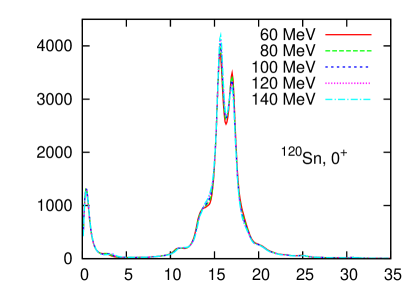
Figure 1: Isoscalar monopole strength function in ¹²⁰Sn. See text for details.

According to these FAM formulae, the residual fields can be calculated by using the finite difference with the parameter $\eta$. In this way, the calculation requires only the HFB Hamiltonian $H[R]$.

Computer programs of the FAM have been developed for spherical nuclei [25] based on the hfbrad [26], and for axially deformed nuclei [27] based on the hfbtho [28]. The FAM in the 3D grid-space representation was also achieved [29, 30] for nuclei in the normal phase. Here, we show the isoscalar monopole strength function in ¹²⁴Sn in Fig. 1. The ground state is obtained by the hfbrad using the SkM* functional and the volume-type pairing. The zero-range nature of the pairing functional requires us to truncate the model space. The truncation was done according to the cutoff for the qp energy, and results with different cutoff energies are shown in Fig. 1 as well. The final results are almost independent from the choice of the cutoff.

5 Canonical-basis TDHFB

In this section, we present another approximate treatment of the TDHFB. Here, we do not take the small amplitude limit, instead, assume the diagonal property of the pair potential. In fact, in the stationary limit, this corresponds to the the well-known BCS approximation for the ground state [15]. Therefore, it can be regarded as the BCS-like approximation in the time-dependent treatment.

At every instant of time, we may identify the canonical basis in which the density is diagonal, $\rho_{ij}(t)=\rho_{i}(t)\delta_{ij}$. The canonical states $(i,\bar{i})$ are always paired with $\rho_{ii}(t)=\rho_{\bar{i}\bar{i}}(t)=\rho_{i}(t)$ and $\kappa_{i\bar{j}}(t)=\kappa_{i}(t)\delta_{ij}$. Here, we introduce an assumption that the pair potential is also diagonal in the canonical basis, $\Delta_{i\bar{j}}=-\Delta_{i}(t)\delta_{ij}$ In the stationary limit, this approximation is identical to the usual BCS approximation [15]. Then, we end up the following set of equations [31].

$$i\frac{\partial}{\partial t}|{i(t)}\rangle=\left\{h(t)-\eta_{i}(t)\right\}|{i(t)}\rangle,\quad\quad i\frac{\partial}{\partial t}|{\bar{i}(t)}\rangle=\left\{h(t)-\eta_{\bar{i}}(t)\right\}|{\bar{i}(t)}\rangle,$$ (26)

$$i\frac{d}{dt}\rho_{i}(t)=\kappa_{i}(t)\Delta_{i}^{*}(t)-\kappa_{i}^{*}(t)\Delta_{i}(t),$$ (27)

$$i\frac{d}{dt}\kappa_{i}(t)=\left\{\eta_{i}(t)+\eta_{\bar{i}}(t)\right\}\kappa_{i}(t)+\Delta_{i}(t)\left\{2\rho_{i}(t)-1\right\}.$$ (28)

Here, $\eta_{i}(t)$ and $\eta_{\bar{i}}(t)$ are arbitrary real functions to control the gauge degrees of freedom of the canonical states. Equations (26), (27), and (28) are invariant with respect to the gauge transformation with arbitrary real functions, $\theta_{i}(t)$ and $\theta_{\bar{i}}(t)$.

$$|{\phi_{i}}\rangle\rightarrow e^{i\theta_{i}(t)}|{\phi_{i}}\rangle\quad \quad|{\phi_{\bar{i}}}\rangle\rightarrow e^{i\theta_{\bar{i}}(t)}|{\phi_{\bar{i}}}\rangle$$ and (29)

$$\kappa_{k}\rightarrow e^{-i(\theta_{i}(t)+\theta_{\bar{i}}(t))}\kappa_{i}\quad \quad\Delta_{k}\rightarrow e^{-i(\theta_{i}(t)+\theta_{\bar{i}}(t))}\Delta_{i}$$ and (30)

simultaneously with

$$\eta_{i}(t)\rightarrow\eta_{i}(t)+\frac{d\theta_{i}}{dt}\quad\mbox{and}\quad\eta_{\bar{i}}(t)\rightarrow\eta_{\bar{i}}(t)+\frac{d\theta_{\bar{i}}}{dt}.$$ (31)

Thus, $\eta_{i}(t)$ and $\eta_{\bar{i}}(t)$, control time evolution of the phases of $|{\phi_{i}(t)}\rangle$, $|{\phi_{\bar{i}}(t)}\rangle$, $\kappa_{i}(t)$, and $\Delta_{i}(t)$.

The canonical-basis TDHFB equations (26), (27), and (28), with a proper gauge choice guarantee the following properties [31]:

1. Conservation law

   1. Conservation of the orthonormal property of the canonical states

   2. Conservation of the average particle number

   3. Conservation of the average total energy

2. The stationary solution corresponds to the HF+BCS state.

3. In the small-amplitude limit, the Nambu-Goldstone modes correspond to zero-energy normal-mode solutions.

In this study, although the method is applicable to the large amplitude dynamics, it is utilized to study the photoreaction of Xe isotopes in the linear regime. Using the instantaneous perturbative external $E1$ field, we calculate the time evolution in the 3D grid-space representation. Then, the Fourier transform of the time-dependent $E1$ moment leads to the $E1$ response function. The smoothing parameter of $\Gamma=1$ MeV is used. See Ref. [31] for numerical details. The calculated $E1$ strength distributions in ^132-140Xe are shown in Fig. 2.

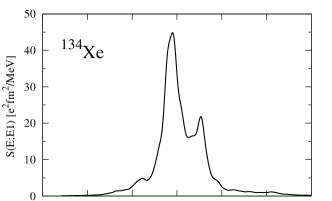
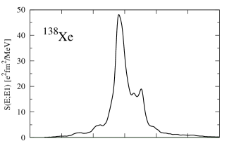
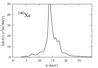
Figure 2: $E1$ strength distributions in Xe isotopes calculated with the SkM* functional.

The ground states of these nuclei are calculated to be spherical, except for ¹⁴⁰Xe which has a very small deformation of $\beta=0.02$. The peak energy of the giant dipole resonance (GDR) is roughly constant and $E_{\rm GDR}\approx 15$ MeV for these isotopes. ¹³⁶Xe corresponds to the neutron magic number $N=82$. The property of the GDR does not significantly depend on the neutron magicity. In the low-energy region below $E=10$ MeV, we may notice an onset of a small dipole peak beyond $N=82$, which appear in ¹³⁸Xe and increases in ¹⁴⁰Xe. This seems to be mainly due to a drastic decrease in the neutron separation energy beyond $N=82$. A systematic study on the low-energy $E1$ strength in this mass region is currently under progress.

It should be emphasized that the computational cost of the present real-time approach is significantly smaller than the normal QRPA calculation based on the diagonalization method. For instance, the computational cost of the QRPA calculation in Ref. [32] is larger than the present one by several orders of magnitude, even though the axial symmetry restriction was utilized. This is because the canonical-basis method utilize the selected canonical states whose number is much smaller than the number of qp states. In addition, the real-time method is very efficient for the present purpose, because the single time evolution produces the nuclear response for the entire energy region.

6 Summary

We presented basic concepts of the density functional theory in nuclear physics, based on the historical developments in nuclear many-body theories. The energy density functional is established as the density-dependent effective interactions, which gives a consistent mean-field-type description of the nuclear saturation property. The time-dependent density functional approach is a powerful method to study dynamics of the quantum many-body systems. In description of heavy open-shell nuclei, the Kohn-Sham orbitals should be extended to the Bogoliubov-type quasiparticle orbitals, to include the pair correlations. This is essentially identical to the TDHFB theory. Although the full treatment of the TDHFB is still a challenging task, we presented approximated treatments; the finite amplitude method and the canonical-basis TDHFB method. Both methods serve as an efficient computational approach to dynamical properties of heavy superfluid nuclei.

References

References

- [1] Bohr A and Mottelson B R 1969 Nuclear Structure vol. 1 (New York; W. A. Benjamin)
- [2] Pieper S C and Wiringa R B 2001 Ann. Rev. Nucl. Part. Sci. 51 53
- [3] Bender M, Heenen P H and Reinhard P-G 2003 Rev. Mod. Phys. 75 121
- [4] Lunney D, Pearson J M and Thibault C 2003 Rev. Mod. Phys. 75 1021
- [5] Hohenberg P and Kohn W 1964 Phys. Rev. B864 136
- [6] Kohn W and Sham L J 1965 Phys. Rev. A1133 140
- [7] Engel J 2007 Phys. Rev. C 75 014306
- [8] Giraud B 2008 Phys. Rev. C 78 014307
- [9] Giraud B, Jennings B K and Barrett B R 2008 Phys. Rev. A 78 032507
- [10] Weizsäcker C F V 1935 Z. Phys. 96 431
- [11] Bethe H A and Bacher R F 1936 Rev. Mod. Phys. 8 82
- [12] Mayer M G and Jensen J H D 1955 Elementary theory of nuclear shell structure (New York: John Wiley & Sons)
- [13] Weisskopf V F 1957 Nucl. Phys. 3 423
- [14] Day B D 1967 Rev. Mod. Phys. 39 495
- [15] Ring p and Schuck P 1980 The nuclear many-body problem (New York; Springer-Verlag)
- [16] Bethe H A and Goldstone J 1957 Proc. Roy. Soc. London A238 551
- [17] Day B D 1981 Phys. Rev. Lett. 47 226
- [18] Negele J W 1970 Phys. Rev. C 1 1260
- [19] Negele J W and Vautherin D 1972 Phys. Rev. C 5 1472
- [20] Vautherin D and Brink D M 1972 Phys. Rev. C 5 626
- [21] Blaizot J-P and Ripka G 1986 Quantum Theory of Finite Systems (Cambridge; MIT Press)
- [22] Hashimoto Y and Nodeki K 2007 Preprint: arXiv:0707.3083
- [23] Stetcu I, Bulgac A, Magierski P and Roche K J 2011 Phys. Rev. C 84 051309
- [24] Nakatsukasa T, Inakura T and Yabana K 2007 Phys. Rev. C 76 024318
- [25] Avogadro P and Nakatsukasa T 2011 Phys. Rev. C 84 014314
- [26] Bennaceur K and Dobaczewski J 2005 Comp. Phys. Comm. 168 96
- [27] Stoitsov M, Kortelainen M, Nakatsukasa T, Losa C and Nazarewicz W 2011 Phys. Rev. C 84 041305
- [28] Stoitsov M V, Dobaczewski J, Nazarewicz W and Ring P 2005 Comp. Phys. Comm. 167 43
- [29] Inakura I, Nakatsukasa T and Yabana K 2009 Phys. Rev. C 80 044301
- [30] Inakura I, Nakatsukasa T and Yabana K 2011 Phys. Rev. C 84 021302
- [31] Ebata S, Nakatsukasa T, Inakura T, Yoshida K, Hashimoto Y and Yabana K 2010 Phys. Rev. C 82 034306
- [32] Terasaki J and Engel J 2010 Phys. Rev. C 82 034326