Non-equilibrium dynamics in Bose-Hubbard ladders

Abstract

Motivated by a recent experiment on the non-equilibrium dynamics of interacting bosons in ladder-shaped optical lattices, we report exact calculations on the sweep dynamics of Bose-Hubbard systems in finite two-leg ladders. The sweep changes the energy bias between the legs linearly over a finite time. As in the experiment, we study the cases of [a] the bosons initially all in the lower-energy leg (ground state sweep) and [b] the bosons initially all in the higher-energy leg (inverse sweep). The approach to adiabaticity in the inverse sweep is intricate, as the transfer of bosons is non-monotonic as a function of both sweep time and intra-leg tunnel coupling. Our exact study provides explanations for these non-monotonicities based on features of the full spectrum, without appealing to concepts (e.g., gapless excitation spectrum) that are more appropriate for the thermodynamic limit. We also demonstrate and study Stückelberg oscillations in the finite-size ladders.

I introduction

The unprecedented experimental tunability of ultra-cold atomic systems in optical potentials provides the opportunity to study non-equilibrium quantum dynamics in previously inaccessible regimes bloch_review ; polkovnikov_review . Very recently, pioneering experiments experiment ; DMRG ; DeMarco_PRL11 have started experimentally exploring issues related to adiabaticity, a fundamental concept of quantum dynamics adiabatic_theorem . Of particular interest is the quantitative characterization of deviations from ideal adiabatic behavior when the sweep rate of a system parameter is small but not infinitesimal. Deviation from adiabaticity in many-body quantum systems has also generated extensive theoretical interest finiteRateQuenches_reviews ; polkovnikov_review . This may be regarded as the slow-sweep counterpart of the much-studied quantum quench (infinite sweep rate) polkovnikov_review .

In the experiment of Ref. experiment , which is the motivation of the present work, adiabaticity is explored through slow ramps of the energy bias (relative potential energy) between two legs of a ladder. The ladder is formed by two coupled one-dimensional tubes or chains. Alternatively, one can think of the experimental setup as a ladder of dimers (double well potentials) coupled to each other, as in Figure 1a. The experimental sequence starts by loading all bosonic atoms in the left leg. The initially filled left leg can be lower in potential energy than the right leg (ground state sweep) or higher (inverse sweep). Subsequently the potential energy is reversed linearly in time, Figure 1b. In a truly adiabatic sweep, i.e., in the limit of large sweep time $\tau$, it is expected that all the bosons get transferred to the right leg. The fraction of particles in the right leg at the end of the sweep, $n_{R}(\tau)$, the so-called transfer efficiency, characterizes adiabaticity.

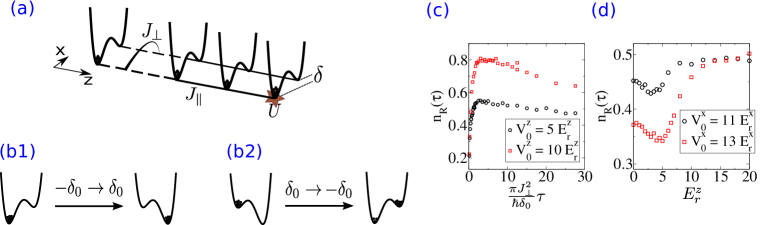
Figure 1: (color online) (a) Each rung of our Bose-Hubbard ladder is a double-well potential (a Bose-Hubbard dimer). Parameters $J_{\perp}$, $J_{\parallel}$, $U$ and $\delta$ are indicated pictorially. (b) Ground state sweep and inverse sweep. The initial state has all bosons on the left site. (c,d) Representative experimental data from Ref. experiment , showing two non-monotonicities of the transfer efficiency $n_{R}(\tau)$. (c) Non-monotonic behavior of $n_{R}(\tau)$ function (“breakdown of adiabaticity”), for different axial $z$-lattice depths. (d) $n_{R}(\tau)$ at a constant value of $\tau$ $\left[\frac{\pi{J_{\perp}^{2}}\tau}{\hbar\delta_{0}}=0.53(3)\right]$ as a function of the axial $z$-lattice depth (roughly: as a function of inverse $J_{\parallel}$), for different inter-tube hoppings.

For the ground state (g.s.) sweep the transfer efficiency increases with sweep time $\tau$, as expected from the quantum adiabatic theorem. In contrast, in the inverse sweep case, after an initial increase $n_{R}(\tau)$ decreases with $\tau$. Following Ref. experiment , we call this non-monotonic behavior a breakdown of adiabaticity. Of course, for extremely slow sweeps (extremely large $\tau$), the adiabatic theorem assures us that $n_{R}(\tau)$ has to increase again to $n_{R}(\tau\rightarrow\infty)=1$. For some $\tau$ values, $n_{R}(\tau)$ also has a non-monotonic dependence on the intra-leg tunnel coupling. The two non-monotonicities are shown through a selection of experimental data (provided by the authors of Ref. experiment ) in Figures 1(c,d).

In this work we analyze exactly the sweep dynamics in small ladder systems. We find that already the smallest system of two bosons in a two-rung ladder shows the two non-trivial non-monotonicities in transfer efficiency, with respect to sweep time and with respect to intra-leg tunneling constant. Analyzing the energy spectra of small ladder systems allows us to explain both effects, and gives us an alternate and useful perspective on the physics involved in sweep dynamics for the Bose-Hubbard ladder and the breakdown phenomenon. The sweep dynamics can be interpreted as a combination of Landau-Zener (LZ) processes LZ through a complex network of avoided level crossings. This exact study allows us to understand the main phenomena without recourse to mean field treatments or low-energy effective descriptions. In addition, small-ladder systems show additional interesting features in the dynamics (Stückelberg oscillations) which are averaged out in larger systems.

In the presence of an overall trapping potential, even if the central ladders are long, there are off-center ladders which consist of a few rungs. Thus, although Ref. experiment focuses on long ladders, the results of the present study should directly describe some part of the experimental measurements performed for Ref. experiment .

We will use the Bose-Hubbard Hamiltonian to describe the system (Figure 1a):

$$\begin{split}H=&-\left(J_{\perp}\sum_{i}b_{i,L}^{\dagger}b_{i,R}+J_{\parallel}\sum_{i,\sigma}b_{i,\sigma}^{\dagger}b_{i+1,\sigma}\right)+\text{h.c.}\\ &+\frac{U}{2}\sum_{i,\sigma}\hat{n}_{i,\sigma}(\hat{n}_{i,\sigma}-1)+\frac{\delta(t)}{2}\sum_{i}(\hat{n}_{i,L}-\hat{n}_{i,R}),\end{split}$$ (1)

where $b_{i,\sigma}$, $b_{i,\sigma}^{\dagger}$ are the bosonic operators for the site on rung $i$ ($i=1\ldots L_{s}$) and leg $\sigma=\text{L, R}$, and $\hat{n}_{i,\sigma}=b_{i,\sigma}^{\dagger}b_{i,\sigma}$. The length of the ladder (number of rungs) is $L_{s}$. The parameters $J_{\perp}$ and $J_{\parallel}$ are the inter-leg and intra-leg tunnel couplings, respectively, $U$ is the on-site interaction energy, and $\delta(t)$ is the time-dependent energy bias between the two legs. We use $J_{\perp}=1$, measuring energy [time] in units of $J_{\perp}$ [$\hbar/J_{\perp}$]. For convenience $\hbar=1$.

The initial state has all bosons on the left leg. In our computation we implement this by taking the initial state to be the ground state of the Hamiltonian (1) with $\delta=-10^{6}$. Thus the initial state of the time evolution is not exactly an eigenstate of the Hamiltonian $H(\delta=\pm\delta_{0})$ at $t=0$, but for relatively large $\delta_{0}$ (we typically use $\delta_{0}$ between 20 and 40), the initial overlap with the relevant eigenstate of $H(t=0)$ is nearly unity.

During a sweep the energy bias between left and right legs is changed linearly in time:

$$\delta(0\leq t\leq\tau)=\begin{cases}\frac{2\delta_{0}}{\tau}t-\delta_{0},&\text{ground state sweep}\\ -\frac{2\delta_{0}}{\tau}t+\delta_{0},&\text{inverse sweep}\end{cases}$$ (2)

where $\tau$ is a sweep time. The dynamics is characterized by the fraction of particles on the right leg

$$n_{R}(t):=N^{-1}\sum_{i}\langle\hat{n}_{i,R}(t)\rangle,$$ (3)

where $N$ is the total number of bosons. In our calculations, the time evolution of the quantum state is obtained by numerical integration of the Schrödinger equation and exact instantaneous eigenvalues and eigenstates of the Hamiltonian (1) are calculated using full numerical diagonalization.

We start in Section II with the sweep dynamics of a single Bose-Hubbard dimer, and show that the g.s. and inverse sweeps have different behaviors already for the dimer. Sections III and IV contain our main results on Bose-Hubbard ladders. Here we identify pertinent features of energy spectra of finite ladders. We present and explain non-monotonic behaviors of the transfer efficiency $n_{R}(\tau)$, observed already in the smallest ladders. In Section V we explain oscillations of $n_{R}(\tau)$ (Stückelberg oscillations), which appear in finite-size ladders but get washed out in the thermodynamic limit. In Section VI we summarize results and mention open problems. In the appendices we describe the treatment of non-interacting Bose-Hubbard ladders and show some results for a larger system.

II Bose-Hubbard dimer

We begin with an $L_{s}=1$ ladder, i.e., a single Bose-Hubbard dimer. Spectral properties and dynamics of the dimer has been studied by various authors (e.g. Milburn ; Kalosakas1 ; Kalosakas2 ; Kalosakas3 ; Salgueiro ; Smerzi1 ; Smerzi2 ; tejaswi ; WuLiu_PRL06 ). Linear sweeps of the energy bias from $-\delta_{0}$ to $0$ were studied in tejaswi in the large $U$ limit. Here, motivated by the expeiments experiment , we focus on small to intermediate $U$ and on the $\pm\delta_{0}\rightarrow\mp\delta_{0}$ sweeps shown in Figure 1b. We will show that the dimer already shows marked difference between ground state sweeps and inverse sweeps, but there is no ‘breakdown’ phenomenon in the inverse sweep.

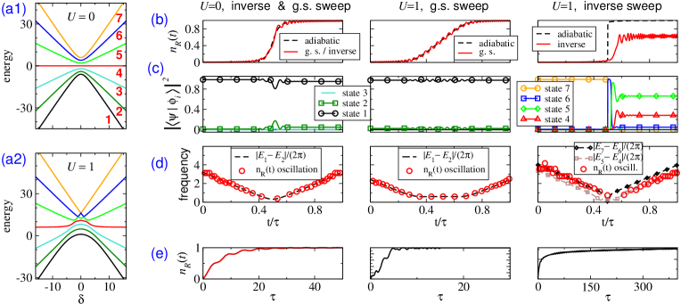
Figure 2: (color online) Spectrum and sweep dynamics of the Bose-Hubbard dimer (single-rung ladder) with $N=6$ bosons. (a) Energy spectrum for $U=0$ and $U=1$. (b,c,d) Sweep dynamics for ($\tau$,$\delta_{0}$) = (40,20). For $U=0$ (first column), g.s. and inverse sweeps are identical. State numbering is shown for g.s sweeps and the inverse sweep simply has states 1,2,… replaced by 7,6,… (b) Population fraction in right site, $n_{R}(t)$. (c) overlap with the instantaneous eigenstates $|\phi_{i}\rangle$. (d) Frequency of oscillations of $n_{R}(t)$, contrasted with differences of instantaneous energy eigenvalues. (e) Transfer efficiency, showing no pronounced non-monotonicity or extended region of decrease.

Figure 2a shows energy spectra for the dimer. There are $N+1$ states. At finite $U$, the states at the top of the spectrum show a cluster of level crossings with tiny gaps, forming a characteristic and well-known swallow-tail shaped structure (e.g. experiment ; odell_PRA11 ; Smerzi_EPJD02 ; WuLiu_PRL06 ; GraefeKorsch_PRA07 ).

Figure 2b shows the time evolution of the right site occupancy for ground state and inverse sweeps, for relatively large sweep time $\tau=40$. In the non-interacting case ground state and inverse sweeps are identical, which is expected because upper and lower parts of the spectrum are equivalent. The adiabaticity is quite good for $\tau=40$, as seen from $n_{R}(t)$ and the overlaps with eigenstates.

For $U>0$ the ground state and inverse sweeps show different behavior. For the g.s. sweep, the adiabaticity is even better at the same $\tau$ than at $U=0$, because the ground state is a bit more separated at $U=1$. In contrast, for the same $\tau$, during the inverse sweep several states become populated by a sequence of Landau-Zener transitions, causing a decrease of boson transfer to the right site. To perform the adiabatic transfer, a sweep has to be carried out much more slower than for a ground state sweep. The reason for this difference is that the energy level structure at the top of the spectrum now contains many level crossings with small gaps.

Oscillations in $n_{R}(t)$ (Figure 2 panels d) are due to occupancy of multiple eigenstates. There are already some oscillations at the beginning of the sweep because the initial state is an eigenstate of $H(\delta=-10^{6})$ and not of $H(\delta=\pm\delta_{0})$. During the sweep, eigenstates other than the lowest/highest get occupied further. Since the energy difference between instantaneous eigenstates (and therefore oscillation frequencies) are changing with time during the sweep, we cannot obtain the frequencies by a Fourier transform of $n_{R}(t)$; in Figure 2 panels d they are approximated from the time difference between successive minima.

The transfer efficiency (Figure 2e) increases monotonically (neglecting oscillations) with $\tau$, for both types of sweep. Thus, in the dimer system inverse sweep dynamics shows no breakdown of adiabaticity, i.e., no pronounced non-monotonicity in $n_{R}(\tau)$.

III Bose-Hubbard ladders

In this section and in section IV we analyze the non-equilibrium sweep dynamics of ladder systems with a few rungs. In this section we describe features of the energy spectrum, show what the sweeps mean in terms of the energy spectrum, and demonstrate that the smallest possible ladder system (two bosons in a two-rung ladder, $L_{S}=N=2$) already displays the two intriguing non-monotonicities that are the main topic of this article. (Non-monotonic dependences of $n_{R}(\tau)$ as a function of $\tau$ and as a function of $J_{\parallel}$, closely analogous to the two non-monotonicities found in Ref. experiment and introduced in Figure 1.) In section IV we provide an explanation of the two non-monotonicities in terms of spectral features and transitions between states of a diabatic basis.

We will use periodic boundary conditions in the leg direction. For a ladder containing only two dimers (rungs), this simply means doubling the intra-leg tunneling constant $J_{\parallel}$. Systems with periodic boundary conditions are translation invariant and the dynamics considered in this paper preserves the total momentum along the leg direction. Since the initial state has zero total momentum, the dynamics is entirely confined to the zero-momentum sector. Thus we use only the subspace of the Hilbert space spanned by the linear combination of the position basis states of the form $1/\sqrt{L_{s}}\sum_{j=0}^{L_{s}-1}T^{j}|n_{1,L},n_{1,R},\dots,n_{L_{s},L},n_{L_{s},R}\rangle$, where $T$ is the translation operator.

III.1 Energy spectrum of Bose-Hubbard ladders

Figure 3 shows energy spectra for $N=3$ bosons in a $L_{s}=3$ (three-rung) ladder. At large $\left|\delta_{0}\right|$, there are $N+1$ groups of states (‘bands’), corresponding to 0,1,2,…,$N$ bosons on the left leg. This is analogous to the dimer which has $N+1$ states. Within each of these bands, the states have splitting (dispersion) determined mainly by the tunneling within the legs, $J_{\parallel}$. For $U=J_{\parallel}=0$, the bands are each degenerate (Figure 3a).

Figure 3b shows that in the $U=0$, $J_{\parallel}\neq 0$ case there are true (unavoided) level crossings (Figure 3d inset). When both $U$ and $J_{\parallel}$ nonzero, the crossings are all avoided (Figure 3d inset). In the sweeps considered in this paper, going from $\pm\delta_{0}$ to $\mp\delta_{0}$, the system wavefunction crosses a complex network of avoided level crossings such as that shown in Figure 3d.

In Figure 4a we show the paths truly adiabatic sweeps would take, for both the g.s. sweep and the inverse sweep. In the two cases, the starting points are the lowest state of the lowest band (g.s. sweep) and the lowest state of the highest band (inverse sweeps).

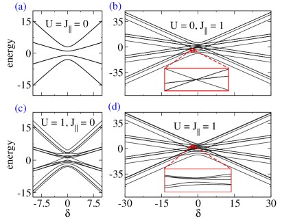
Figure 3: (color online) Energy spectra of Bose-Hubbard ladder for $L_{s}=N=3$ in zero momentum subspace. (a) $U=J_{\parallel}=0$: the eigenstates are degenerate. (b) $J_{\parallel}=1,U=0$: each band splits into eigenstates with different kinetic energy. Level crossings are real (not avoided) crossings, as shown in inset. (c) $U=1,J_{\parallel}=0$: the on-site interaction splits the eigenstates within each band. (d) $J_{\parallel}=U=1$: all crossings in the spectrum are avoided, as shown in the inset.

III.2 Sweeps and adiabaticity in few-rung ladders

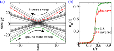
Figure 4: (color online) (a) Energy spectrum in zero momentum subspace for $L_{s}=3$, $N=4$, $U=1$, $J_{\parallel}=0.4$, with 42 levels. The adiabatic paths for g.s. and inverse sweeps are highlighted. (b) Fraction of bosons on the right leg $n_{R}(t)$ as function of time, during sweeps with ($\delta_{0}$,$\tau$) = (20,40). For the g.s. sweep the $n_{R}(t)$ reaches nearly unity, following the adiabatic path closely. In contrast, after the inverse sweep $n_{R}(t)$ falls far short of unity, even with a sweep as slow as $\tau=40$.

As we found for the dimer, in Bose-Hubbard ladders interactions are necessary for seeing a difference in adiabaticity between ground state and inverse sweep. In the appendix A, we provide analytical calculations for non-interacting ($U=0$) ladders where the g.s. and inverse sweeps are identical and there is no breakdown phenomenon.

In this subsection and the rest of the main text, we will consider finite interactions. For $U\neq 0$ ladders, the g.s. and inverse sweeps are different (as for the dimer), and in addition there is also the breakdown phenomenon. In this subsection, we present the main features of the non-equilibrium dynamics in few-rung Bose-Hubbard ladders during linear sweeps of the energy bias, and also present the main features of the transfer efficiency.

Figure 4b shows the time dependence of the boson fraction on the right leg $n_{R}(t)$, for a $\tau=40$ sweep. For this sweep time, the ground state sweep exhibits almost adiabatic behavior, while the inverse sweep deviates significantly. This difference is similar to that described for the dimer (single-rung ladder) in section II. Compared to the dimer, the fundamentally new feature in the ladder system is seen in the dependence of $n_{R}(\tau)$ on the sweep time $\tau$, which is non-monotonic and shows a pronounced region of decrease with increasing $\tau$. This is displayed in Figure 5.

Oscillations in $n_{R}(t)$ complicate the behavior of the transfer efficiency $n_{R}(\tau)$. So, after the sweep, we evolve the final state with the time independent final Hamiltonian $H(t=\tau)$ over a large additional time, to get the time-averaged transfer efficiency $\overline{n}_{R}(\tau):=\langle n_{R}(t>\tau)\rangle_{t}$.

Figure 5 shows $\overline{n}_{R}(\tau)$ as a function of the sweep time $\tau$ and of the intra-leg tunnel coupling $J_{\parallel}$ for inverse sweeps in the smallest non-trivial ladder ($L_{s}=N=2$). The transfer efficiency exhibits non-monotonicities as function of both $\tau$ and $J_{\parallel}$. For faster sweeps $\overline{n}_{R}(\tau)$ increases with increasing $\tau$. In contrast, in the slow sweep regime ($\tau\gtrsim 20$), $\overline{n}_{R}(\tau)$ decreases with increasing $\tau$ for $J_{\parallel}\gtrsim{0.2}$. In addition, for $\tau\gtrsim 20$, the transfer efficiency at fixed $\tau$ also depends non-monotonically $J_{\parallel}$. These two non-monotonicities are analogs of those observed in experiment (Figure 1), and are analyzed in detail in the next section. Compared to the larger systems considered in Ref. DMRG , we have additional oscillatory features, analyzed in section V.

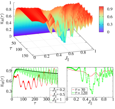
Figure 5: (color online) Transfer efficiency $\overline{n}_{R}(\tau)$ as function of the sweep time $\tau$ and the intra-leg hopping $J_{\parallel}$ for inverse sweep, for the “minimal” ladder $L_{s}=N=2$ and $U=1,\delta_{0}=30$. Non-monotonicities with respect to both $\tau$ and $J_{\parallel}$ are visible in the 3D plot, and are also shown separately in 2D panels.

IV The non-monotonic behavior of the transfer efficiency

In this section we provide microscopic explanations of the two non-monotonicities of the transfer efficiency $\overline{n}_{R}(\tau)$ shown in Figure 5. The explanations are based on considerations of the structure of energy spectra of Bose-Hubbard ladders and the couplings between energy levels. The $\tau$ non-monotonicity can be understood by neglecting the crossing structure in the small $|\delta|$ regime of the spectrum and only examining the coupling matrix elements between the large-$|\delta|$ states. This will be explained first in IV.1. The $J_{\parallel}$ non-monotonicity arises from features of the crossing structure of the spectrum and is described in IV.2.

IV.1 Non-monotonicity with sweep time

In this subsection we describe the microscopic origin of the non-monotonic behavior of the $\overline{n}_{R}(\tau)$ function (breakdown of adiabaticity). We will detail an analysis for the simplest case of $L_{s}=N=2$ (two bosons in two-rung ladder, Figure 6), and extract the general explanation from this special case. In terms of the state numbering in Figure 6, adiabaticity in the inverse sweep involves starting at state 5 on the left and populating state 1 on the right. ‘Breakdown’ involves a non-monotonic dependence on $\tau$ of the final state 1 population. We therefore examine and explain the overlaps of the final wavefunction with the final eigenstates, as a function of $\tau$.

The details of the crossing structure of the spectrum at small $|\delta|$ (ellipse in Figure 6a) vary widely with Hamiltonian parameters (c.f. Figure 3). On the other hand, the breakdown effect is robust through a large region of parameter space. This suggests that the phenomenon can be explained ignoring the exact crossing structure of the spectrum around $\delta=0$. Our strategy is therefore to use the states at large $\delta$ as a ‘diabatic’ basis and examine the coupling matrix among these states.

Diabatic representation: The spectrum (Figure 6a) consists of three bands of two states each, and the initial state is very close to the lowest state of the highest band, i.e. state 5.

The time evolution starts and ends at $|\delta(t=\{0,\tau\})|\gg 1$, where the Hamiltonian (1) is dominated by the energy bias term $\delta/2\sum_{i}(\hat{n}_{i,L}-\hat{n}_{i,R})$. If one regards the on-site interaction ($U$) and the inter-leg hopping ($J_{\perp}$) terms as couplings, then in analogy to the two-level Landau-Zener problem the eigenstates of the Hamiltonian with $U=J_{\perp}=0$ can be regarded as the diabatic basis. The spectrum of the coupling free Hamiltonian $H_{J_{\perp}=U=0}$ is shown in Figure 6b. The diabatic basis can be calculated analytically using the procedure described in Appendix A for treating non-interacting Hamiltonians.

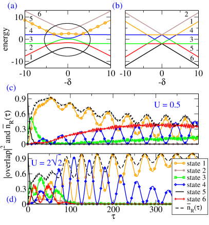
Figure 6: (color online) (a) Spectrum of minimal ladder ($L_{s}=N=2$), with $J_{\parallel}=0.5,U=1$. The adiabatic path for inverse sweep (5 $\rightarrow$ 1) is highlighted with circles. The crossing structure for small $|\delta|$ is indicated by an ellipse. Since $\delta(t=0)>0$ we use $-\delta$ on the horizontal axis so that the sweep goes from left to right. (b) The diabatic basis states, obtained by setting $U=J_{\perp}=0$. (c) Overlap of the final state with the eigenstates of the final Hamiltonian and transfer efficiency. Same parameters as in panel (a); $\delta_{0}=30$. System goes into state 1 for fast sweeps, but population of state 1 is reduced with increasing $\tau$ in favor of ‘band-excited’ states 4 and 6. (d) Larger interaction, for which there is no breakdown. The final population of state 1 increases monotonically (neglecting oscillations) with $\tau$.

For large energy bias $|\delta|\gg 1$ the eigenstates of the full Hamiltonian coincide with the diabatic states. The coupling strengths between diabatic states sets the probability for transition between these states. Loosely speaking, this means the overlap of the final wavefunction with a diabatic state after the sweep is larger when the coupling (either direct or higher-order) with the initial state is larger. In other words, a transition with larger coupling should be noticeable already for faster sweeps (smaller $\tau$), while states weakly coupled would need a slower sweep to get populated.

The coupling matrix between the diabatic states is obtained by representing the full Hamiltonian in the diabatic basis:

$$\begin{pmatrix}-&\frac{U}{2}&-\sqrt{2}J_{\perp}&0&0&0\\ \frac{U}{2}&-&0&-\sqrt{2}J_{\perp}&0&0\\ -\sqrt{2}J_{\perp}&0&-&0&-\sqrt{2}J_{\perp}&0\\ 0&-\sqrt{2}J_{\perp}&0&-&0&-\sqrt{2}J_{\perp}\\ 0&0&-\sqrt{2}J_{\perp}&0&-&\frac{U}{2}\\ 0&0&0&-\sqrt{2}J_{\perp}&\frac{U}{2}&-\\ \end{pmatrix}.$$

The diabatic basis states are ordered according to the numbering of Figure 6. We note that states from neighboring bands with same kinetic energy along the ladder (i.e., states $1;3;5$ and states $2;4;6$) are coupled by $J_{\perp}$. States from the same band, if coupled, are coupled through the interaction $U$. We will next show how these observations on coupling terms allow an explanation of the breakdown phenomenon, and also allow us to predict regions of parameter space where the phenomenon does not occur.

Breakdown of adiabaticity: In Figure 6c we show the final overlaps as a function of $\tau$, for a parameter combination for which breakdown is exhibited. At fast ramp rates (small $\tau$), the states at the bottom of bands (states 1,3) get occupied, so that the occupancy of state 1 (and hence $\overline{n}_{R}(\tau)$) increases to a maximum. For slower sweeps, the occupancy of these states is lost to higher-momentum states in lower bands, (states 4,6). This decrease of state 1 occupancy (and hence of $\overline{n}_{R}(\tau)$) is the breakdown phenomenon. The same description holds for larger ladders (which have more bands and more states in each band) — (a) the band ground states are successively occupied at small times, so that the $\overline{n}_{R}(\tau)$ and the lowest state of the highest band increase initially with $\tau$, and (b) for slower ramps excited states of lower bands gain weight at the expense of the highest band g.s. These processes are illustrated for a larger system in Figure 7.

We can explain this in terms of two different coupling strengths (different time scales) for initial excitation of the highest band ground state (state 1) and for later transfer to excited states of lower bands. In the $L_{s}=N=2$ case, this relies on $\frac{1}{2}U$ being smaller than $\sqrt{2}J_{\perp}$, and for larger ladders we would require $U$ to be smaller than $c_{1}J_{\perp}$ for some constant $c_{1}$. The lowest states of successive bands can get populated with coupling strength $J_{\perp}$, so that the time scale for initially populating the ‘adiabatic’ final state (state 1) is set by ${\sim}J_{\perp}^{N}$. The time scale for moving to excited states of lower bands is however set by the weaker coupling ${\sim}J_{\perp}^{N-1}U$, and is thus slower, and can happen only for slower sweeps. This explains the loss of state 1 occupancy in favor of excited states of lower bands, at larger $\tau$.

Population of band excited states is fundamental to the breakdown mechanism. This corresponds to the idea of longitudinal low-lying excitations (gapless phonon excitations) along legs, highlighted in Ref. experiment . Note that our microscopic mechanism above does not rely on any idea of gapless excitations, which strictly speaking only occurs in infinitely long ladders.

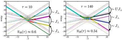
Figure 7: (color online) Spectra for $L_{s}=N=3$, $J_{\parallel}=U=1$, showing time evolution during inverse sweeps ($\delta_{0}=30$) through overlaps, which are indicated by line widths. The width of lines is $\sim\ln(\text{overlap})$, and if the overlap is smaller than 2% the line is dashed. Transfer efficiency has a maximum at $\tau=40$, $\overline{n}_{R}(\tau)=0.87$. As argued in text, we see that for small $\tau$ (left) the main process is the successive excitation of band ground states. In the breakdown regime (right), the higher states of lower bands are excited. Arrows highlight this mechanism pictorially.

Parameter regimes without breakdown of adiabaticity: A strong confirmation of our picture is the absence of breakdown at larger $U$, as shown in Figure 6d. For larger $U$, the time scale for populating lower-band excited states is comparable or smaller than the time scale for initial population of higher-band ground state. Not having a slower time scale, there is no longer any mechanism for $\overline{n}_{R}(\tau)$ decrease with $\tau$.

Another regime with no breakdown is that of small $J_{\parallel}$. A simple way to understand this is that, for $J_{\parallel}\rightarrow 0$, the system corresponds to isolated single dimers, and we have seen in section II that the phenomenon is an absent in a single dimer.

IV.2 Non-monotonicity with intra-leg hopping

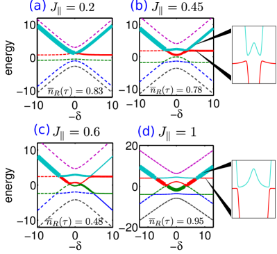
Figure 8: (color online) Time evolution during inverse sweep in the minimal ladder ($L_{s}=N=2$), shown through overlaps indicated by line widths. The width of lines is $\propto$ overlap, and if the overlap is smaller than 5% the line is dashed. Here $U=1$, $\tau=200$, $\delta_{0}=20$. Insets on right show blowups of the crossings in energy spectra, in the same scale, highlighting the differences between small and large $J_{\parallel}$.

To explain the non-monotonicity of $\overline{n}_{R}(\tau)$ with $J_{\parallel}$ at moderately large $\tau$, we now consider the crossing structure of the energy spectrum at small $|\delta|$ and how this structure changes with $J_{\parallel}$. Figure 8 shows this for the minimal ($L_{s}=N=2$) ladder.

For very small $J_{\parallel}$ (Figure 8a) the bands have little or no overlap, so the lowest state of the highest band has little or no proximity to any other energy level during the sweep. As a result, the transfer efficiency is large for moderate $\tau$.

As $J_{\parallel}$ is increased, the width of each band increases, resulting in multiple crossings, in particular between the lowest state of the highest band and various excited states of lower bands (Figures 8b and 8c). Via these crossings, the wavefunction can populate states of lower bands, leading to loss of transfer efficiency.

When $J_{\parallel}$ is increased even further (Figure 8d), the crossings happen at larger $|\delta|$ and have smaller gaps. (Physically, the gaps are smaller at larger $|\delta|$ because the diabatic states are more sharply different and hence mix less.) Small-gap crossings behave more like true crossings. Thus at large $J_{\parallel}$ and moderate $\tau$ the main path taken by the wavefunction ends up at the lowest level of the highest band, even though this path passes through many crossings, as shown in Figure 8d.

To summarize, increasing $J_{\parallel}$ has two effects: at first it increases the number of crossings, which reduces the transfer efficiency, and then for even larger $J_{\parallel}$ it makes the crossing gaps smaller, which again increases the transfer efficiency. This explains the overall minimum in the $\overline{n}_{R}(\tau)$ versus $J_{\parallel}$ behavior. Of course, the behavior is complicated by interference effects (Stückelberg oscillations), prominent in the lower right panel of Figure 5. In Figure 8 we have chosen four $J_{\parallel}$ values that highlight the overall trend of the $\overline{n}_{R}(\tau)$ versus $J_{\parallel}$ behavior.

V Stückelberg oscillations

In this section we analyze the oscillations observed in the transfer efficiency (Figures 5, 6, and 9a). While the overall trends discussed previously reflect the macroscopic physics which is the focus of Refs. experiment ; DMRG , the oscillations are particular to our microscopic (small-system) ladders.

When a system is swept through a parameter region containing multiple avoided level crossings, the wavefunction may split into two eigenstates at one crossing and, later in the sweep, levels with nonzero weight may meet again and interfere. Such interference can lead to oscillatory behavior of observables as a function of the sweep rate Stuckelberg_interferometry . The wavefunction component following the energy level $E_{i}$ will accumulate the phase $\int{E_{i}}dt$. As a result, in quantities like $\overline{n}_{R}(\tau)$ there are interference terms carrying phase factors of type $\int\left[E_{i}-E_{j}\right]dt$, for each pair of levels ($i$,$j$) with nonzero weight. Since the sweeps change $\delta$ linearly in time, $dt=-\frac{\tau}{2\delta_{0}}\text{d}\delta$. Thus the phase factors are

$$\frac{\tau}{2\delta_{0}}\int\left[E_{i}(\delta)-E_{j}(\delta)\right]\text{d}\delta=\frac{A_{\alpha}}{2\delta_{0}}\tau$$ (4)

where $A_{\alpha}$’s are the areas enclosed between levels and crossings in the energy-$\delta$ plane, as shown in Figure 9c inset. Thus the oscillations as a function of $\tau$ carry frequency $A_{\alpha}/2\delta_{0}$.

In Figure 9b the Fourier spectrum of $\overline{n}_{R}(\tau)$ is shown. There are three pronounced peaks. These frequencies can be compared to “enclosed areas” in the energy spectrum diagram (Figure 9c inset). Figure 9c shows excellent agreement between the oscillation frequencies, obtained by Fourier analysis, and the exact numerically calculated areas $A_{\alpha}$ multiplied by $\frac{1}{2\delta_{0}}$.

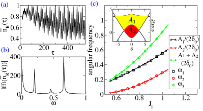
Figure 9: (color online) Stückelberg oscillations in minimal ladder ($L_{s}=N=2$), with $\delta_{0}=20$, $U=1$, $J_{\parallel}=0.85$. (a,b) Transfer efficiency $\overline{n}_{R}(\tau)$ and its Fourier transform. (c) Frequencies compared to areas enclosed by crossing lines in the spectrum. Inset shows relevant region of spectrum and definitions of areas.

VI Summary and Conclusion

A recent experiment with trapped bosonic atoms in ladder-shaped optical lattices has highlighted the intricacies that can arise in the approach to adiabaticity in interacting systems experiment ; DMRG . Motivated by this experiment, we have undertaken an exact study of Bose-Hubbard ladders of explicitly finite size. We have thoroughly examined the energy spectra, their crossings, and the transitions between them, and explained some non-trivial features of the transfer efficiency.

The understanding emerging from this analysis is that, while interaction effects are vital for the “breakdown of adiabaticity” and related effects, the thermodynamic limit is not at all necessary for understanding the main effects qualitatively. In particular, the two non-trivial non-monotonicities are both well-explained without appealing to concepts like gapless-ness of excitation spectra or nonlinearities in mean-field descriptions.

The present analysis opens up various avenues of possible future research. Since a trapped system contains ladders of all possible sizes, one might ask whether from the data one can extract information relevant to the sizes we have considered here, in particular whether it is possible to study the interference features (Stückelberg oscillations) which are prominent in small ladders. Second, non-equilibrium dynamics in the size regime between the present sizes and large sizes remains unexplored. This relates to the widely appreciated difficulty of interpolating between full quantum treatments of small systems and mean-field treatments of larger systems.

Appendix A Non-interacting Bose-Hubbard ladder

With periodic boundary conditions (translation invariance), the time dependence of the $U=0$ Bose-Hubbard ladder of arbitrary length can be reduced to a single 2x2 system, i.e., a single Landau-Zener type problem.

Writing the Hamiltonian (1) with $U=0$ in momentum space, one can diagonalize using a unitary transformation for every momentum mode ($q=0,\ldots,L_{s}-1$):

$$\begin{split}&\alpha_{q}=u_{q}\cdot a_{q,L}+v_{q}\cdot a_{q,R}\\ &\beta_{q}=v_{q}\cdot a_{q,L}-u_{q}\cdot a_{q,R},\end{split}$$ (5)

with $u^{2}+v^{2}=1$. The diagonalization condition yields $u/v=2J_{\perp}/\delta$, and the resulting diagonal Hamiltonian is

$$\begin{split}H^{U=0}=&\sum_{q}\bigg{[}-2J_{\parallel}\cos(\frac{2\pi}{L_{s}}q)(\alpha^{\dagger}_{q}\alpha_{q}+\beta_{q}^{\dagger}\beta_{q})\\ &+\frac{\delta}{|\delta|}\frac{1}{2}\sqrt{\delta^{2}+4J_{\perp}^{2}}(\beta_{q}^{\dagger}\beta_{q}-\alpha^{\dagger}_{q}\alpha_{q})\bigg{]}.\end{split}$$ (6)

The eigenstates can now be created by applying $\alpha_{q}^{\dagger}$, $\beta_{q}^{\dagger}$ operators on the vacuum, e.g., the ground state at negative $\delta$ is $|\psi_{g.s.}\rangle=\frac{1}{\sqrt{N!}}(\beta_{0}^{\dagger})^{N}|0\rangle$. Dynamics is obtained using Heisenberg equations of motion for the $\beta_{q}$ operator, which leads to the same 2x2 problem for each $q$ mode:

$$i\hbar\begin{pmatrix}\dot{v}\\ \dot{u}\end{pmatrix}=\begin{pmatrix}\frac{\delta(t)}{2}-2J_{\parallel}&-J_{\perp}\\ -J_{\perp}&-\frac{\delta(t)}{2}-2J_{\parallel}\end{pmatrix}\begin{pmatrix}v\\ u\end{pmatrix}$$ (7)

The fraction of bosons in the right leg is $n_{R}(t)=|u(t)|^{2}$. The 2x2 dynamics is too simple for $n_{R}(t)$ to display any of the nontrivial behaviors we have studied in the main text with nonzero interactions. For large $\delta_{0}$ and $\tau$, we can use the Landau-Zener formula to calculate the transfer efficiency: $n_{R}(\tau)=1-\exp[-2\pi{J_{\perp}^{2}}/\alpha]$, with $\alpha=\pm 2\frac{\delta_{0}}{\tau}$. Of course, this increases monotonically with $\tau$.

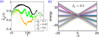
Figure 10: (color online) (a) Breakdown of adiabaticity in larger system. $L_{s}=5$, $N=4$, $U=1$, $\delta_{0}=20$. (b) Time evolution during an inverse sweep in the breakdown regime ($\tau=80$. $J_{\parallel}=0.5$), presented (as in Figures 7 and 8) through the line-widths representing overlap ($\sim\ln(\text{overlap})$).

Appendix B $L_{s}=5,N=4$

In Figure 10 the breakdown of adiabaticity is shown for a larger system containing four bosons in five-dimer ladder. The Stückelberg oscillations in $\overline{n}_{R}(\tau)$ are now far less pronounced, but otherwise the features of the breakdown phenomenon are very similar to those presented in detail for smaller systems in the main text. The overlaps of Figure 10b show that band excited states, corresponding to longitudinal modes along the leg directions, are excited in the breakdown process, consistent with the picture developed in section IV.1.

References

- (1) I. Bloch, J. Dalibard, and W. Zwerger, Rev. Mod. Phys. 80, 885 (2008).
- (2) A. Polkovnikov, K. Sengupta, A. Silva and M. Vengalattore, Rev. Mod. Phys. 83, 863 (2011).
- (3) Y.-A. Chen, S. D. Huber, S. Trotzky, I. Bloch, and E. Altman, Nature Physics 7, 61 (2011).
- (4) C. Kasztelan, S. Trotzky, Y.-A. Chen, I. Bloch, I. P. McCulloch, U. Schollwöck, and G. Orso, Phys. Rev. Lett. 106, 155302 (2011).
- (5) D. Chen, M. White, C. Borries, and B. DeMarco, Phys. Rev. Lett. 106, 235304 (2011).
- (6) P. Ehrenfest, Ann. Phys. 51, 327 (1916); M. Born and V. Fock, Z. Phys. 512, 165 (1928); T. Kato, J. Phys. Soc. Jap. 5, 435 (1950); M. H. S. Amin, Phys. Rev. Lett. 102, 220401 (2009).
-
(7)
See reviews and citations of earlier work in:
J. Dziarmaga, Adv. Phys. 59, 1063 (2010);
Chapters 2-5 in Quantum Quenching, Annealing and Computation, edited by A. K. Chandra, A. Das, and B. K. Chakrabarti, Springer, 2010; - (8) L. D. Landau, Phys. Z. Sowjetunion 2, 46 (1932); C. Zener, Proc. R. Soc. London, Ser. A 137, 696 (1932).
- (9) G. J. Milburn, J. Corney, E. M. Wright, and D. F. Walls, Phys. Rev. A 55, 4318 (1997).
- (10) G. Kalosakas and A. R. Bishop, Phys. Rev. A 65, 043616 (2002).
- (11) G. Kalosakas, A. R. Bishop, and V. M. Kenkre, Phys. Rev. A 68, 023602 (2003).
- (12) G. Kalosakas, A. R. Bishop, and V. M. Kenkre, J. Phys. B 36, 3233 (2003).
- (13) A. N. Salgueiro, A. F. R. de Toledo Piza, G. B. Lemos, R. Drumond, M. C. Nemes, and M. Weidemueller, Eur. Phys. J. D44, 537 (2007).
- (14) S. Raghavan, A. Smerzi, S. Fantoni, and S. R. Shenoy, Phys. Rev. A 59, 620 (1999).
- (15) S. Raghavan, A. Smerzi, and V. M. Kenkre, Phys. Rev. A 60, R1787 (1999).
- (16) T. Venumadhav, M. Haque, and R. Moessner, Phys. Rev. B 81, 054305 (2010).
- (17) B. Wu and J. Liu, Phys. Rev. Lett. 96, 020405 (2006).
- (18) F. Mulansky, J. Mumford, and D. H. J. O’Dell, Phys. Rev. A 84, 063602 (2011).
- (19) Z. P. Karkuszewski, K. Sacha, and A. Smerzi, Eur. Phys. J. D 21, 251 (2002).
- (20) E. M. Graefe and H. J. Korsch, Phys. Rev. A 76, 032116 (2007).
- (21) E. C. G. Stückelberg, Helv. Phys. Acta. 5, 369 (1932). S. N. Shevchenko, S. Ashhab, and F. Nori, Physics Reports 492, 1 (2010).