Topology of Minimal Walking Technicolor

Abstract

We perform a lattice study of the topological susceptibility and instanton size distribution of the $\mathrm{SU}(2)$ gauge theory with two adjoint Dirac fermions (also known as Minimal Walking Technicolor), which is known to be in the conformal window. In the theory deformed with a small mass term, by drawing a comparison with the pure gauge theory, we find that topological observables are decoupled from the fermion dynamics. This provides further evidence for the infrared conformality of the theory. A study of the instanton size distribution shows that this quantity can be used to detect the onset of finite size effects.

1 Introduction

After the recent experimental breakthroughs that allowed the announcement of the discovery of a new bosonic particle with mass at the electroweak scale atlas2012gk ; cms2012gu , the focus of experiments is moving towards the determination of the nature of this boson, with the goal of finding hints for new physics. Hence, it is of utmost importance for theorists to investigate possible scenarios of electroweak symmetry breaking beyond the standard model. An appealing possibility is the existence of a new strong interaction whose chiral condensate breaks electroweak symmetry. Based on this idea, over the years a physically consistent framework denoted as Walking Techinicolor (WT) was developed Weinberg1975gm ; Susskind1978ms ; Eichten1979ah ; Holdom1981rm ; Holdom1984sk ; Yamawaki1985zg ; Appelquist1986an ; Miransky1996pd ; Dietrich2006cm ; Dietrich2006ck (reviews on the topic include Hill2002ap ; Piai2010ma ; Andersen2011yj ). In order to be consistent with the stringent electroweak precision measurements, a theory realising the WT scenario must have two crucial properties: dynamics characterised by near-conformality, and a chiral condensate with anomalous dimension of order one. In most semi-analytical treatments of WT, both properties are taken as reasonable assumptions. In order to prove that there exist realistic gauge theories characterised by near-conformal behaviour and large anomalous dimension, calculations from first principles are needed. Gauge-string duality techniques can be used to engineer theories with the required properties in the limit in which the number of gauge bosons goes to infinity (see e.g. Nunez2008wi ; Elander2009pk ; Kutasov2012uq ; Levkov2012yk ; Anguelova2012ka ; Clark2012pm and references therein). For a gauge theory based on a finite Lie group, lattice computations provide the best quantitative tool.

In recent years, a large body of activity has been devoted by the lattice community to computations aimed at characterising the phases of gauge theories, with the goal of understanding signatures of the conformal and near-conformal regime. The current understanding is summarised in Neil2012cb . Among the theories investigated to date, $\mathrm{SU}(2)$ with two Dirac fermions in the adjoint representation (also known as Minimal Walking Technicolor Sannino:2004qp ; Dietrich:2005jn ; Foadi:2007ue , for which experimental constraints have been recently reported in atlas-mwt ) plays an important role: it is the only theory studied so far to show unambiguously the expected behaviour of an infrared conformal theory, in independent numerical results obtained with different techniques and targeting different observables. Although for building a technicolor model one needs a near-conformal gauge theory, first principle studies of infrared conformal theories are interesting both from a theoretical point of view and from a phenomenological perspective Luty2004ye . After the first exploratory calculations of physical quantities in this theory Catterall2007yx ; DelDebbio2008zf ; Catterall2008qk ; Hietanen2008mr , which were fundamental in ascertaining its conformal behaviour, lattice studies have focussed on the running of the coupling near the fixed point Hietanen2009az ; Bursa2009we ; DeGrand2011qd ; Catterall2011zf , on the calculation of the anomalous dimension of the chiral condensate Lucini2009an ; DelDebbio2009fd ; DelDebbio2010hu ; DelDebbio2010hx ; Giedt2012rj ; Patella2012da and more recently on controlling finite size effects Karavirta2011mv ; Bursa2011ru ; DelDebbio2011kp . The main goals of this community effort have been to establish a reliable technique to extract the anomalous dimension and to identify a good set of observables that could provide an unambiguous signature of conformal behaviour. These investigations are expected to be relevant also for the near-conformal case, in which the theory will mimic the properties of a conformal theory at some intermediate distances before showing its true confining and chiral symmetry breaking nature at asymptotically large distances.

To date, the attention of lattice studies has focussed on spectral quantities. In this paper, we shall report on a first investigation of topological quantities, and in particular on the behaviour of the topological charge, of the instanton size distribution and of the topological susceptibility. These quantities play an important role in confining and chiral symmetry breaking theories like QCD (see e.g. Delia2012vv for a recent work), but their behaviour in (near-)conformal gauge theories has not been explored before. We shall study whether those observables can be used to identify the infinite volume regime and the scaling regime in the mass-deformed theory. Taking inspiration from the perturbative argument given in Miransky1998dh , in DelDebbio2009fd it has been shown from first principles that $\mathrm{SU}(2)$ gauge theory with two Dirac adjoint flavours behaves like a confining theory with heavy adjoint quarks for any finite value of the fermion mass, which plays the role of a deforming parameter in a would-be infrared conformal theory. Hence, in the infinite volume limit, we expect topological observables to be compatible with those of Yang-Mills, with any small deviation originating from the fermionic matter, and large deviations being due to finite size effects. The decoupling of instantons in the chiral limit has been discussed also in Sannino:2008pz .

The purpose of this investigation is twofold. On the one hand, we aim to verify that for large volumes topological variables are broadly compatible with Yang-Mills values and at characterising qualitatively their behaviour on smaller volumes. On the other hand, we want to investigate whether an accurate value for the anomalous dimension of the condensate can be extracted from topological observables. The rest of the paper is organised as follows. In Sect. 2 we review the formulation of the theory of interest on the lattice and we define the observables related to topological quantities that are studied in this work. Our numerical results are reported in Sect. 3, with discussions of methods for extracting the anomalous dimension of the condensate delegated to Sect. 4. Finally, Sect. 5 summarises the main findings of our study.

2 Methodology

In this work, we study the theory on an four-dimensional Euclidean spacetime lattice. The lattice discretisation used here is described in DelDebbio2008zf . We recall the main points below, referring to DelDebbio2008zf for further details.

On the lattice, the dynamics of the gauge variables is described by group elements in the fundamental representation living on the links of the lattice. If $U_{\mu}(i)$ is the field living on the link originating from the lattice point $i$ in the direction $\hat{\mu}$, the plaquette operator $U_{\mu\nu}(i)$ is defined as

$$U_{\mu\nu}(i)=U_{\mu}(i)U_{\nu}(i+\hat{\mu})U_{\mu}^{{\dagger}}(i+\hat{\nu})U_{\nu}^{{\dagger}}(i)\ .$$ (1)

In $\mathrm{SU}(N)$, the Wilson action for the gauge degrees of freedom of the theory is then

$$S_{\mathrm{g}}=\beta\sum_{i,\mu,\nu}\left(1-\frac{1}{2N}\mbox{Tr}\left(U_{\mu\nu}(i)+U_{\mu\nu}^{{\dagger}}(i)\right)\right)\ ,$$ (2)

with $\beta=1/g^{2}$ and $g$ the gauge coupling. In the Wilson formulation, which is the discretisation used in our work, the dynamics of the fermions is described by the Dirac operator $M_{\alpha\beta}(ij)$, defined as

$$M_{\alpha\beta}(ij) = (m+4r)\delta_{ij}\delta_{\alpha\beta}-\frac{1}{2}\left[\left(r-\gamma_{\mu}\right)_{\alpha\beta}U^{\mathrm{R}}_{\mu}(i)\delta_{i,j-\hat{\mu}}\right.$$ (3)

$$\quad+\left.\left(r+\gamma_{\mu}\right)_{\alpha\beta}\left(U^{\mathrm{R}}_{\mu}(i)\right)^{{\dagger}}\delta_{i,j+\hat{\mu}}\right]\ ,$$

where $i$ and $j$ are lattice sites and $\alpha$ and $\beta$ Dirac indices. The superscript $\mathrm{R}$ indicates that the link variable have to be taken in the representation of the fermions and $m$ is the bare fermion mass. Since this fermion discretisation breaks chiral symmetry, the chiral point has to be determined non-perturbatively in the numerical simulation. A possible definition of this point uses the fermion mass $m_{\mathrm{PCAC}}$ defined through the partially conserved axial current: the chiral limit is attained at the point for which $m_{\mathrm{PCAC}}$ is zero.

With those definitions, the lattice discretised version of the $\mathrm{SU}(2)$ gauge theory with two adjoint fermions we are studying is described by the path integral

$$Z=\int\left({\cal D}U_{\mu}(i)\right)(\det M(U_{\mu}))^{N_{\mathrm{f}}}e^{-S_{\mathrm{g}}}\ ,$$ (4)

where the link variables are $\mathrm{SU}(2)$ matrices, $M$ is in the adjoint representation and the number of flavours $N_{\mathrm{f}}$ is 2. A set of configurations that dominate the path integral can be generated with Monte Carlo methods, and vacuum expectation values of observables are computed as ensemble averages of the corresponding operators over those configurations. These observables have a relative statistical fluctuation that scales as $1/\sqrt{N_{\mathrm{s}}}$, where $N_{\mathrm{s}}$ is the number of the generated configurations. Thus the numerical error can be kept systematically under control by adjusting the size of the sample.

The observables we have studied are described in smith-teper , to which we refer for further details about the observables and the model assumptions made to derive the relationships we use in our work. Here we only summarise the main points. In the continuum, the topological charge density can be expressed as

$$Q(x)=\frac{1}{32\pi^{2}}\epsilon_{\mu\nu\rho\sigma}\mathrm{Tr}\left\{F_{\mu\nu}(x)F_{\rho\sigma}(x)\right\}\ .$$ (5)

The total topological charge of a configuration can then be obtained as the integral of this quantity over the spacetime.

The equivalent lattice topological charge density is then given by:

$$Q_{\mathrm{L}}(i)=\frac{1}{32\pi^{2}}\epsilon_{\mu\nu\rho\sigma}\mathrm{Tr}\left\{U_{\mu\nu}(i)U_{\rho\sigma}(i)\right\}\ .$$ (6)

For a smooth gauge field, this would have fluctuations of order $a^{2}$ as the lattice spacing $a$ is sent to zero; however, realistic fields have ultraviolet fluctuations which will completely dominate over the physics of interest in the continuum limit. To mitigate this, a cooling process is introduced Teper1985rb . The cooling process operates by minimising the local action for each lattice site in turn. Successive cooling sweeps will “smooth out” the fluctuations such that the physics may be observed. A side effect however is that instantons may be shrunk or may annihilate in instanton–anti-instanton pairs, thus excessive cooling is to be avoided. The number of cooling sweeps performed in a calculation results from the compromise between the need to smooth out the configurations and the necessity of not losing physical instantons by annihilation. The tuning of this parameter is not critical, since there is a wide plateau where the physics can be observed before cooling artefacts set in.

Once the topological charge density is known, various observables may be calculated. The topological susceptibility is defined as

$$\chi_{\mathrm{T}}=\frac{\left\langle Q_{\mathrm{T}}^{2}\right\rangle-{\left\langle Q_{\mathrm{T}}\right\rangle}^{2}}{V}\ ,$$ (7)

where $V$ is the lattice volume and $Q_{\mathrm{T}}$ is the total topological charge, defined as

$$Q_{\mathrm{T}}=\sum_{i}Q_{\mathrm{L}}(i)\ ,$$ (8)

with $i$ running over all lattice points. Since in the continuum the total topological charge is an integer, on the lattice $Q_{\mathrm{T}}$ is often rounded to the nearest integer. Alternative discretisations can be used. Lattice studies (e.g. lucini-teper ; Alles:1997nu ) show that the particular definition of $Q_{\mathrm{T}}$ does not affect the results if the calculation is done close to the continuum limit, as one would have expected.

The size of a given instanton may be calculated from the local maxima of the absolute value of the topological charge density given in Eq. (6) from the relation

$$q_{\mathrm{peak}}=\frac{6}{\pi^{2}\rho^{4}}\ ,$$ (9)

which has been used to determine the instanton size distribution and the average instanton size.

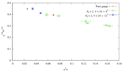
Figure 1: Variation of the quantity $\chi^{\frac{1}{4}}/\sqrt{\sigma}$ with $a^{2}\sigma$. Smaller string tensions corresponds to smaller fermion masses.

3 Results

Preexisting two-flavour configurations discussed in DelDebbio2010hx (to which we refer for measurements of spectral quantities and for a careful discussion of finite volume artefacts) were used, at $\beta=2.25$, with $V=16\times 8^{3}$, $m=-0.90$, $-0.75$, $-0.50$, $-0.25$, $0.00$, $0.25$, $0.50$ and $V=24\times 12^{3}$, $m=-1.00$, $-0.95$. 20 cooling sweeps were used for all configurations. For comparison with the Yang-Mills case, pure gauge configurations were generated at $\beta=2.4,V=12^{4}$ and $\beta=2.55,V=20^{4}$; each update consisted of 1 heat bath and 4 over-relaxation steps, and measurements were taken every 10th and 50th configuration on the smaller and larger lattice respectively. At each $\beta$, the size of the lattice has been chosen so that finite size effects for spectral observables are negligible, with the linear size of the lattice (in physical units) being around 1.5 fm in both cases lucini-teper (for the conversion to fm, we have assumed $\sqrt{\sigma}=420$ MeV). Our numerical results have been obtained with a bootstrap procedure over the data divided in bins of 20 measurements each.

Before discussing our findings, it is important to note that, although apparently similar from an operational point of view and for scope and results, the comparison with the pure gauge results (which is an important part of this work) is conceptually different from a comparison with quenched data in QCD with heavy quarks: in the latter theory, a large quark mass only slightly modifies the string tension, and its effect can be reabsorbed with a shift in $\beta$. Here (see Refs. DelDebbio2009fd ; DelDebbio2010hu ; DelDebbio2010hx ) when the (small) fermion mass is varied towards the chiral limit, a variation of the value of the string tension by an order of magnitude is induced on $\sigma$. Since the lattice spacing is not changing ($\beta$ is kept fixed across the various values of the mass), the interpretation (consistent with calculations around the Caswell-Banks-Zaks Caswell1974 ; Banks:1981nn fixed point) is that it is the scale of the long-distance effective Yang-Mills theory that changes as a result of varying the mass. As a consequence, a comparison with the Yang-Mills theory entails the matching of the quantity $a\sqrt{\sigma}$. For this reason, even if in the dynamical theory we are at fixed $\beta$, for the comparison one has to choose a different value of the coupling in the pure gauge theory for each value of the fermion mass in the dynamical theory.

Table 1: Numerical results for $m_{PCAC}$, $\chi$ and $\overline{\rho}$ as a function of $m$ on lattices of size $2L\times L^{3}$. Note that we have removed the point at $m=0.50$ from plots making use of $\sigma$, owing to the unavailability of a reliable value of $\sigma$ for this data set.

$aL$	$m$	$am_{\mathrm{PCAC}}$	$a^{4}\chi$	$\overline{\rho}/a$
8	$-0.90$	0.4330(18)	$8.23(17)\times{10}^{-5}$	4.12(67)
8	$-0.75$	0.5607(18)	$1.365(23)\times{10}^{-4}$	4.02(51)
8	$-0.50$	0.7224(13)	$1.764(28)\times{10}^{-4}$	3.96(41)
8	$-0.25$	0.8552(11)	$2.059(33)\times{10}^{-4}$	3.88(37)
8	$\phantom{-}0.00$	0.9706(11)	$2.188(37)\times{10}^{-4}$	3.86(35)
8	$\phantom{-}0.25$	1.07205(97)	$2.141(35)\times{10}^{-4}$	3.85(34)
8	$\phantom{-}0.50$	1.16353(73)	$2.198(36)\times{10}^{-4}$	3.84(34)
12	$-1.00$	0.33623(82)	$6.502(93)\times{10}^{-5}$	6.18(94)
12	$-0.95$	0.39017(68)	$4.772(81)\times{10}^{-5}$	5.73(67)

We start with the topological susceptibility. For this quantity, we have used the integer definition of $Q_{\mathrm{T}}$, after having verified that alternative definitions give compatible results. Our findings (reported in table 1 and plotted in figure 1) show consistency between the pure gauge and the 2-flavour theory, as one would have expected. As a check, we have verified that our pure gauge results are consistent with those presented in lucini-teper .

Figure 2: Instanton size distribution for the two-flavour configuration sets and for the pure gauge configuration sets at the values of the lattice parameters shown.

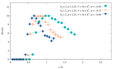
Figure 3: Instanton size distribution in the dynamical case on the smaller lattice at the parameters shown. The appearance of a peak at larger instanton size signals the onset of finite size artefacts.

Although no sign of finite size effects can be seen in the topological susceptibility, there are visible hints of them in the instanton size distribution. We start our discussion by comparing this observable in the pure gauge case and in the two flavour theory on the larger lattice. The instanton size distribution (figure 2, showing the distributions of instantons of physical size $\rho\sqrt{\sigma}$) has a similar behaviour, characterised by a peak and a large size tail, whose end is possibly affected by finite size artefacts. When going from larger to smaller string tensions, the evolution of the shape of the distribution in the dynamical case seems to be compatible with the quenched one. This behaviour is consistent with the distribution found in studies of the same quantity in other contexts instanton-size-1 ; instanton-size-2 ; instanton-size-3 . However, on the smaller lattice, as the fermion mass is decreased, value, the $N_{\mathrm{f}}=2$ theory shows a sharper peak, a position of the peak moved towards smaller sizes and a longer tail (figure 3). This signals the onset of finite volume artefacts. If one avoids the region in which lattice artefacts are dominant, when rescaled in units of $\sqrt{\sigma}$, the instanton size distribution on different lattice volumes shows the same large-size behaviour, while at smaller instanton sizes the distribution on the smaller lattice is suppressed (figure  4). We ascribe this suppression to more prominent cooling artefacts that cause instantons to shrink below the lattice spacing on smaller lattices.

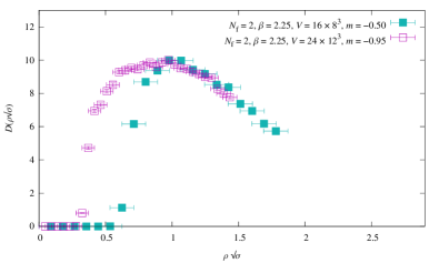
Figure 4: Comparison between the instanton size distributions for the dynamical case at the smaller and larger lattice volume, for the sets of bare parameters shown.

4 Anomalous dimension and scaling

In a conformal gauge theory, for which the fermion mass is the only relevant coupling at the infrared fixed point, at large distances and in the infinite volume limit all observables scale with an exponent related to their naïve mass dimension and to the anomalous dimension of the condensate. Let us consider a multiplicatively renormalised mass $m$ such that the chiral limit is attained at $m=0$ (like for instance the PCAC mass). If $\gamma^{\ast}$ is the anomalous dimension of the condensate, at leading order in $m$ an observable $O$ with mass dimension $d_{O}$ scales as

$$O\propto m^{d_{O}/(1+\gamma^{\ast})}\ .$$ (10)

The argument parallels the derivation of scaling relations of statistical systems at criticality and assumes that the correlation length of the system is the only relavant scale DeGrand2009mt . This assumption is known as the hyperscaling hypothesis.

Infinite volume scaling relations emerge as the large size limit of finite size scaling, which in turn can be derived by adding the size of the system, $L$, to the set of relevant couplings Lucini2009an ; DelDebbio2010hx ; DelDebbio2010jy ; DelDebbio2010ze . Hence, for a finite system of size $L$, Eq. (10) becomes

$$OL^{d_{O}}=F_{O}(Lm^{1/(1+\gamma^{\ast})})\ ,$$ (11)

where $F_{O}$ is a universal function of of the scaling variable $x=Lm^{1/(1+\gamma^{\ast})}$. At large $L$ and small $x$,

$$F_{O}=x^{d_{O}}+\dots\ ,$$ (12)

and Eq. (11) reduced to Eq. (10).

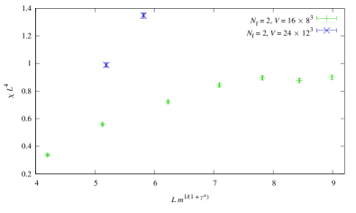
Figure 5: Rescaling of the topological susceptibility data according to Eq. (14) with $\gamma^{\ast}=0.3$.

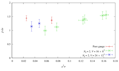
Figure 6: Variation of the average instanton size with $\sigma$.

As a consequence of scaling and finite volume scaling arguments, under the assumption that the marginal $\theta$-term operator does not generate sizeable scaling violations, in the large volume and small mass regime, the topological susceptibility $\chi$ will show the scaling behaviour

$$\chi\propto m^{\frac{4}{1+\gamma^{\ast}}}\ .$$ (13)

At finite but large volume $L^{4}$, this relationship becomes

$$\chi=L^{-4}F_{\chi}(Lm^{1/(1+\gamma^{\ast})})\ ,$$ (14)

with $F_{\chi}$ universal function of $Lm^{1/(1+\gamma^{\ast})}$ in the limits $L\to\infty$ and $m\to 0$. Analogously, the instanton size distribution follows the scaling and finite size scaling laws

$$\overline{\rho} = Am^{-1/(1+\gamma^{\ast})}\ ,$$ (15)

$$\overline{\rho} = LF_{\overline{\rho}}(Lm^{1/(1+\gamma^{\ast})})\ ,$$ (16)

respectively, with $A$ in Eq. (15) a constant.

We performed a fit of the topological susceptibility data according to Eqs. (13) and (14), but we did not see the expected scaling. Even putting a reasonable bound on $\gamma^{\ast}$ proves to be hard with the current data: adjusting by hand the value of $\gamma^{\ast}$ in the range 0.0–1.0 did not result in any universal behaviour as a function of the scaling variable. An example is provided in figure 5.

The average instanton size is reported in table 1 and plotted in figure 6. This quantity shows qualitative scaling and a behaviour compatible with the pure gauge case. However, the relatively large error on $\overline{\rho}$ does not allow to extract an accurate value for the anomalous dimension: an acceptable scaling is obtained for $0\leq\gamma^{\ast}\leq 2$.

While the lack of precision in the determination of $\gamma^{\ast}$ from $\overline{\rho}$ is due to the intrinsical difficulties in measuring reliably this observable, the most plausible explanation for the apparent absence of scaling in $\chi$ is that larger lattices are required in order for the scaling behaviour to manifest. Although this could have been expected from previous studies, in Patella2012da it was shown an example of an observable that has precocious scaling. Our analysis shows that this is not the case for the topological susceptibility. Generating configurations in the scaling region of gluonic observables requires a big computational effort, which is outside the scope of this work. Currently, a calculation in this direction is being performed DelDebbio2011kp . These newly generated configurations will allow us to investigate the scaling of the topological susceptibility as the mass goes to zero in the appropriate range of volumes and then to answer the question of whether the topological suceptibility is an efficient observable to extract the anomalous dimension.

5 Conclusions

In this work, we performed the first numerical investigation of the behaviour of instanton-related quantities in a mass-deformed infrared conformal gauge theory. For the theory we have studied, $\mathrm{SU}(2)$ gauge theory with two dynamical adjoint Dirac fermions, we found that the behaviour of the topological susceptibility supports the scenario in which the infrared dynamics is dominated by gluonic quantities, with the fermions being more massive Miransky1998dh ; DelDebbio2009fd (see also Sannino:2008pz ). Moreover, the instanton size distribution provides a good indication of finite volume effects. We plan to extend this study to larger lattices, in order to check whether the topological susceptibility obeys the expected scaling with the mass and whether we can extract from it the anomalous dimension of the condensate. Finally, it would be interesting to apply those techniques to other theories that could provide a realisation of the walking scenario, like e.g. $\mathrm{SU}(3)$ gauge theory with two sextet fermions DeGrand2012yq ; Holland2012fu .

- (1) G. Aad, et al., Phys.Lett.B (2012). DOI 10.1016/j.physletb.2012.08.020
- (2) S. Chatrchyan, et al., Phys.Lett.B (2012). DOI 10.1016/j.physletb.2012.08.021
- (3) S. Weinberg, Phys. Rev. D13, 974 (1976). DOI 10.1103/PhysRevD.13.974
- (4) L. Susskind, Phys. Rev. D20, 2619 (1979). DOI 10.1103/PhysRevD.20.2619
- (5) E. Eichten, K.D. Lane, Phys. Lett. B90, 125 (1980). DOI 10.1016/0370-2693(80)90065-9
- (6) B. Holdom, Phys.Rev. D24, 1441 (1981). DOI 10.1103/PhysRevD.24.1441
- (7) B. Holdom, Phys. Lett. B150, 301 (1985). DOI 10.1016/0370-2693(85)91015-9
- (8) K. Yamawaki, M. Bando, K.i. Matumoto, Phys. Rev. Lett. 56, 1335 (1986). DOI 10.1103/PhysRevLett.56.1335
- (9) T.W. Appelquist, D. Karabali, L.C.R. Wijewardhana, Phys. Rev. Lett. 57, 957 (1986). DOI 10.1103/PhysRevLett.57.957
- (10) V. Miransky, K. Yamawaki, Phys.Rev. D55, 5051 (1997). DOI 10.1103/PhysRevD.56.3768, 10.1103/PhysRevD.55.5051
- (11) D.D. Dietrich, F. Sannino, Phys.Rev. D75, 085018 (2007). DOI 10.1103/PhysRevD.75.085018
- (12) D.D. Dietrich, F. Sannino, Phys. Rev. D75, 085018 (2007). DOI 10.1103/PhysRevD.75.085018
- (13) C.T. Hill, E.H. Simmons, Phys. Rept. 381, 235 (2003). DOI 10.1016/S0370-1573(03)00140-6
- (14) M. Piai, Adv. High Energy Phys. 2010 (4302). DOI 10.1155/2010/464302
- (15) J. Andersen, O. Antipin, G. Azuelos, L. Del Debbio, E. Del Nobile, et al., Eur.Phys.J.Plus 126, 81 (2011). DOI 10.1140/epjp/i2011-11081-1
- (16) C. Nunez, I. Papadimitriou, M. Piai, Int. J. Mod. Phys. A25, 2837 (2010). DOI 10.1142/S0217751X10049189
- (17) D. Elander, C. Nunez, M. Piai, Phys. Lett. B686, 64 (2010). DOI 10.1016/j.physletb.2010.02.023
- (18) D. Kutasov, J. Lin, A. Parnachev, Nucl.Phys. B863, 361 (2012). DOI 10.1016/j.nuclphysb.2012.05.025
- (19) D. Levkov, V. Rubakov, S. Troitsky, Y. Zenkevich, arXiv:1201.6368 (2012)
- (20) L. Anguelova, P. Suranyi, L.R. Wijewardhana, Nucl.Phys. B862, 671 (2012). DOI 10.1016/j.nuclphysb.2012.05.005
- (21) T. Clark, S. Love, T. ter Veldhuis, arXiv:1208.0817 (2012)
- (22) E.T. Neil, PoS LATTICE2011, 009 (2011)
- (23) F. Sannino, K. Tuominen, Phys.Rev. D71, 051901 (2005). DOI 10.1103/PhysRevD.71.051901
- (24) D.D. Dietrich, F. Sannino, K. Tuominen, Phys.Rev. D72, 055001 (2005). DOI 10.1103/PhysRevD.72.055001
- (25) R. Foadi, M.T. Frandsen, T.A. Ryttov, F. Sannino, Phys.Rev. D76, 055005 (2007). DOI 10.1103/PhysRevD.76.055005
- (26) G. Aad, et al., arXiv:1209.2535 (2012)
- (27) M.A. Luty, T. Okui, JHEP 0609, 070 (2006). DOI 10.1088/1126-6708/2006/09/070
- (28) S. Catterall, F. Sannino, Phys. Rev. D76, 034504 (2007). DOI 10.1103/PhysRevD.76.034504
- (29) L. Del Debbio, A. Patella, C. Pica, Phys. Rev. D81, 094503 (2010). DOI 10.1103/PhysRevD.81.094503
- (30) S. Catterall, J. Giedt, F. Sannino, J. Schneible, JHEP 11, 009 (2008). DOI 10.1088/1126-6708/2008/11/009
- (31) A.J. Hietanen, J. Rantaharju, K. Rummukainen, K. Tuominen, JHEP 0905, 025 (2009). DOI 10.1088/1126-6708/2009/05/025
- (32) A.J. Hietanen, K. Rummukainen, K. Tuominen, Phys. Rev. D80, 094504 (2009). DOI 10.1103/PhysRevD.80.094504
- (33) F. Bursa, L. Del Debbio, L. Keegan, C. Pica, T. Pickup, Phys. Rev. D81, 014505 (2010). DOI 10.1103/PhysRevD.81.014505
- (34) T. DeGrand, Y. Shamir, B. Svetitsky, Phys.Rev. D83, 074507 (2011). DOI 10.1103/PhysRevD.83.074507
- (35) S. Catterall, L. Del Debbio, J. Giedt, L. Keegan, Phys.Rev. D85, 094501 (2012). DOI 10.1103/PhysRevD.85.094501
- (36) B. Lucini, Phil.Trans.Roy.Soc.Lond. A368, 3657 (2010). DOI 10.1098/rsta.2010.0030
- (37) L. Del Debbio, B. Lucini, A. Patella, C. Pica, A. Rago, Phys.Rev. D80, 074507 (2009). DOI 10.1103/PhysRevD.80.074507
- (38) L. Del Debbio, B. Lucini, A. Patella, C. Pica, A. Rago, Phys.Rev. D82, 014509 (2010). DOI 10.1103/PhysRevD.82.014509
- (39) L. Del Debbio, B. Lucini, A. Patella, C. Pica, A. Rago, Phys. Rev. D 82, 014510 (2010). DOI 10.1103/PhysRevD.82.014510. URL http://link.aps.org/doi/10.1103/PhysRevD.82.014510
- (40) J. Giedt, E. Weinberg, Phys.Rev. D85, 097503 (2012). DOI 10.1103/PhysRevD.85.097503
- (41) A. Patella, Phys.Rev. D86, 025006 (2012). DOI 10.1103/PhysRevD.86.025006
- (42) T. Karavirta, A. Mykkanen, J. Rantaharju, K. Rummukainen, K. Tuominen, JHEP 1106, 061 (2011). DOI 10.1007/JHEP06(2011)061
- (43) F. Bursa, L. Del Debbio, D. Henty, E. Kerrane, B. Lucini, et al., Phys.Rev. D84, 034506 (2011). DOI 10.1103/PhysRevD.84.034506
- (44) L. Del Debbio, B. Lucini, A. Patella, C. Pica, A. Rago, PoS LATTICE2011, 084 (2011)
- (45) D. Nogradi, JHEP 1205, 089 (2012). DOI 10.1007/JHEP05(2012)089
- (46) P. de Forcrand, M. Pepe, U.J. Wiese, arXiv:1204.4913 (2012)
- (47) M. D’Elia, F. Negro, Phys.Rev.Lett. 109, 072001 (2012). DOI 10.1103/PhysRevLett.109.072001
- (48) V. Miransky, Phys.Rev. D59, 105003 (1999). DOI 10.1103/PhysRevD.59.105003
- (49) F. Sannino, Phys.Rev. D80, 017901 (2009). DOI 10.1103/PhysRevD.80.017901
- (50) D.A. Smith, M.J. Teper, Phys. Rev. D 58, 014505 (1998). DOI 10.1103/PhysRevD.58.014505. URL http://link.aps.org/doi/10.1103/PhysRevD.58.014505
- (51) M. Teper, Phys.Lett. B162, 357 (1985). DOI 10.1016/0370-2693(85)90939-6
- (52) B. Lucini, M. Teper, JHEP 0106, 050 (2001). DOI 10.1088/1126-6708/2001/06/050
- (53) B. Alles, M. D’Elia, A. Di Giacomo, R. Kirchner, Phys.Rev. D58, 114506 (1998). DOI 10.1103/PhysRevD.58.114506
- (54) W.E. Caswell, Phys. Rev. Lett. 33, 244 (1974). DOI 10.1103/PhysRevLett.33.244. URL http://link.aps.org/doi/10.1103/PhysRevLett.33.244
- (55) T. Banks, A. Zaks, Nucl.Phys. B196, 189 (1982). DOI 10.1016/0550-3213(82)90035-9
- (56) M. García Pérez, T.G. Kovács, P. van Baal, Phys.Lett. B472, 295 (2000). DOI 10.1016/S0370-2693(99)01451-3
- (57) C. Michael, P. Spencer, Phys.Rev. D52, 4691 (1995). DOI 10.1103/PhysRevD.52.4691
- (58) S. Hands, P. Kenny, Phys.Lett. B701, 373 (2011). DOI 10.1016/j.physletb.2011.05.065
- (59) T. DeGrand, A. Hasenfratz, Phys. Rev. D80, 034506 (2009). DOI 10.1103/PhysRevD.80.034506
- (60) L. Del Debbio, R. Zwicky, Phys.Lett. B700, 217 (2011). DOI 10.1016/j.physletb.2011.04.059
- (61) L. Del Debbio, R. Zwicky, Phys. Rev. D82, 014502 (2010). DOI 10.1103/PhysRevD.82.014502
- (62) T. DeGrand, Y. Shamir, B. Svetitsky, arXiv:1201.0935 (2012)
- (63) K. Holland, Z. Fodor, J. Kuti, D. Nogradi, C. Schroeder, et al., arXiv:1209.0391 (2012)