Long-range correlations of neutrinos in hadron reactions and neutrino diffraction II:  neutrino

Abstract

In this II, a probability to detect the neutrino produced in a high-energy pion decay is shown to receive the large finite-size correction. The neutrino interacts extremely weakly with matters and is described with a many-body wave function together with the pion and charged lepton. This wave function slowly approaches to an asymptotic form, which is probed by the neutrino. The whole process is described by an S-matrix of a finite-time interval, which couples with states of non-conserving kinetic energy, and the final states of a broad spectrum specific to a relativistic invariant system contribute to the positive semi-definite correction similar to diffraction of waves through a hole. This diffraction component for the neutrino becomes long range and stable under changes of the pion’s energy. Moreover, it has a universal form that depends on the absolute neutrino mass. Thus a new method of measuring the absolute neutrino mass is suggested.

Department of Physics, Faculty of Science,

Hokkaido University, Sapporo 060-0810, Japan

1 Introduction

The method of computing the finite-size correction developed in I [1] is applied to the probability to detect neutrinos in pion decay. Since a neutrino, charged lepton, and pion are described by a many-body wave function that follows Schrödinger equation, the kinetic energy at a finite time is not a constant and takes a wide range of values, as was shown in I. Consequently these waves include broad spectrum and show a diffraction phenomenon that is non-uniform in space-time. Since the speed of light is an accumulation point of the relativistic waves, a two-point correlation function has the light-cone singularity and the probability to detect the neutrino is subject to a finite-size correction. The neutrinos are very light and propagate with almost the light speed, hence the correction becomes unusual and depends, in fact, on absolute neutrino masses which are not found from oscillation experiments. Thus the correction becomes extremely large in its magnitude and size and has universal properties for the neutrino.

Tritium beta decays [2] have been used for determining the absolute value but an existing upper bound for an effective electron neutrino mass-squared is of the order of $2~{}[\text{eV}^{2}/c^{4}]$ and the mass is $0.3-1.3~{}[\text{eV}/c^{2}]$ from cosmological observations [3]. In these neutrino experiments, higher precision and more statistics have been achieved and will be improved more.

Weak decay processes have been studied using an S-matrix of plane waves with asymptotic boundary conditions, where particles in the initial and final states are regarded as free waves without correlations [4, 5, 6, 7, 8]. A decay rate, average life time, and various distributions of charged leptons have been computed, and perfect agreements with experiments have been obtained [9]. These facts proved that the standard theory of electro-weak interaction is correct.

Neutrinos have almost the light speed and are detected at a distant position, hence they are similar to an electrostatic potential of a moving body, which has a finite-size correction in a form of a retarded potential. Due to its extremely small mass, the probability to detect the neutrino may depend on the distance between a source and observation positions. To study position-dependent probabilities, the standard S-matrix of plane waves that satisfies a boundary condition at $t=\pm\infty$, which gives the values at the asymptotic regions, is useless. An S-matrix that satisfies boundary conditions at a finite-time interval T, $S[\text{T}]$, and has a position dependence is appropriate. Because boundary conditions for $S[\text{T}]$ are different from those of $S[\infty]$, it reveals different properties form those of $S[\infty]$. We compute the finite-size corrections of transition probabilities with $S[\text{T}]$ expressed by wave packets. The wave packets vanish at a position ${\vec{x}}$ if the distance between ${\vec{x}}$ and the center position ${\vec{X}}$, $|{\vec{x}}-{\vec{X}}|\rightarrow\infty$, and satisfy the boundary conditions of the experiments [7, 8]. Hence they are appropriate to study the finite-size effect and are used here [10, 11, 12].

A pion is produced in a proton reaction first and decays next. The whole process is expressed in Fig. 1 of I. The first reaction caused by strong interactions was studied in I and the second reaction caused by weak interactions is studied in II. From I, a particle in the final state retains the wave nature in the region of $r\leq l_{0}$, where $r$ is a distance between the initial sates and final state and a coherence length $l_{0}$ in a high-momentum region, $|\vec{p}|\gg m$, is given by

$$l_{0}=\left({2|\vec{p}\,|\hbar c\over m^{2}}\right),$$ (1)

where $m$ is the particle’s mass and becomes for a neutrino of mass $1$ [eV/$c^{2}$] and energy $1$ [GeV]

$$l_{0}^{neutrino}={2\hbar c\over 1^{2}}\times 10^{18}[\text{GeV}^{-1}]=10^{2}-10^{3}[\text{m}],$$ (2)

Thus $l_{0}$ of neutrino are macroscopic lengths. Hence a measurement of neutrino process at a near-detector region may depend on a distance $|{\vec{X}}-{\vec{X}}^{(i)}|$, where ${\vec{X}}$ and ${\vec{X}}^{(i)}$ are the positions of the nucleus in the detector and target.

Detecting neutrinos at ${\vec{X}}$ of a distance ${|{\vec{X}}-{\vec{X}}^{(i)}|\gg l_{0}}$ is studied in a usual manner. Since the neutrino in this region is expressed by a plane wave that behaves like a free particle, the neutrino’s number and flux behave like those of classical particles and the production and detection of the neutrino are treated separately. The neutrino flux is determined by its distribution functions of the number and velocity that are determined by the decay process and is used for calculation of the scattering processes.

Measurements in ${|{\vec{X}}-{\vec{X}}^{(i)}|\leq l_{0}}$, on the other hand, are not treated by particle dynamics but by wave dynamics. The entire processes should be taken into account and be studied either by time-dependent Schrödinger equations or by position-dependent amplitudes defined with wave packets. The wave packets are necessary to measure the quantities in this region. Since the particles are identified based on signals generated by their interactions with a nucleus, atom, or larger system of matter, this unit of detector has a finite size and is expressed by wave packets. Using wave packet representations, the amplitude of detecting neutrinos in a pion decay is computed. The probability to detect the neutrino depends on the distance $|{\vec{X}}-{\vec{X}}^{(i)}|$, hence a naive neutrino flux is not defined uniquely. The uniform flux defined by the classical particles is necessarily constant and is not used here. It might be reasonable to define the flux here based on the number of events that the neutrino gives rise to. The probabilities can be computed relatively easily with a set of simple wave packets such as Gaussian wave packets and are equivalent in more general wave packets. Although they depend upon not only the distance but also the wave packet size, they have universal properties. So it would make sense to define a neutrino flux from the probability computed with the Gaussian wave packet. Thus we define the neutrino flux in this region from the probability to detect the neutrino. The idea is similar to define the electric field from a force that a point particle receives. The finite-size effects are actually large in the processes of detecting neutrinos at a macroscopic distance. Thus the corrections are important when the theoretical values are compared with the experimental values.

Fig. 1: The geometry of the pion decay region and the neutrino detector. The neutrino is produced in the pion decay and is detected. Since the decay position is not fixed to one value but is arbitrary, the amplitude to detect the neutrino is the overlap between the superposed initial wave and a final state expressed by the wave packet of the small size. The neutrino observed by the detector at $T_{\nu}$ shows an interference pattern.

It is instructive to see how a single neutrino interference is observed. A neutrino produced in a pion decay propagates a finite distance before it is detected. A position where a neutrino is produced varies, so a neutrino wave at the detector is a superposition of those waves that are produced at different space-time positions. If these space-time positions are inside of one pion, as in Fig. 1, the waves keep their coherence and reveal interference patterns. A condition for the interference phenomenon to occur, for one dimensional motion of the pion that keeps a coherence within the region $\sqrt{\sigma_{\pi}}$ and a velocity $\vec{v}_{\pi}$ is obtained in the following manner. Let a neutrino be produced either at time $t_{1}$ or $t_{2}$ from the pion prepared at $\text{T}_{\pi}$ and travel for some period and be finally detected at $\text{T}_{\nu}$, then the waves overlap if

$$|(c(\text{T}_{\nu}-t_{1})+v_{\pi}(t_{1}-\text{T}_{\pi}))-(c(\text{T}_{\nu}-t_{2})+v_{\pi}(t_{2}-\text{T}_{\pi}))|\leq\sqrt{\sigma_{\pi}},$$ (3)

is met, where the speed of light is used for the speed of neutrino $v_{\nu}=c$. So Eq. $(\ref{coherence-condition})$ is one of the necessary conditions for the neutrino interference to occur in the one-dimensional space. For a plane wave of pion $\sigma_{\pi}=\infty$ and the above condition is satisfied. For a high-energy pion of a finite $\sigma_{\pi}$, its speed is close to the speed of light and the left hand side of Eq. $(\ref{coherence-condition})$ becomes $c(m_{\pi}^{2}/2E_{\pi}^{2})(t_{1}-t_{2})$. Hence this condition Eq. $(\ref{coherence-condition})$ is written in the form, $c(t_{1}-t_{2})\leq\sqrt{\sigma_{\pi}}(2E_{\pi}^{2}/m_{\pi}^{2})$. When this length $c(t_{1}-t_{2})$ is a macroscopic size, the interference phenomenon occurs at a macroscopic length. We estimated the lengths of these particles in Appendix of I and confirmed that this condition in three-dimensional space is fulfilled in a macroscopic distance.

An amplitude to detect a neutrino is an integral of a product of wave functions of a pion, muon, and neutrino and a velocity of a space-time position of transition of the pion to the muon has a component of the light velocity and the neutrino has almost the light velocity. Hence they overlap in wide space-time area and the amplitude and probability to detect the neutrino get a contribution of a large interference effect. A neutrino flux becomes distinct from the naive value obtained from the standard method of using an incoherent probability.

This paper is organized in the following manner. In section 2, we study an amplitude of detecting a neutrino in a pion decay process and compute a position-dependent probability in section 3. For a rigorous calculation of the position-dependent probability, a correlation function is introduced. Using an expression with the correlation function and its singular structure at a light-cone region, the finite-size correction is computed in section 4. Implication to neutrino experiments, features of the finite-size corrections, and summary and prospects are given in section 5, 6, and 7.

2 Position-dependent amplitude of neutrino

Position-dependent probabilities of detecting a neutrino and a charged lepton in a pion decay process are computed with a Schrödinger equation at a finite time $t$ and an S-matrix of a finite-time interval T. They have various properties different from those at the infinite time. Especially the final states in ultraviolet energy regions couple and give a finite and universal contribution.

A neutrino or a charged lepton is detected with a detector that is located in a macroscopic distance from the position of the initial pion. Since their properties are determined from their probabilities in experiments, the whole process is studied. The process is described with a many-body wave function of the pion and decay products. The neutrino and charged lepton in the final state is highly correlated with the pion in the initial state and have a kinetic energy different from the initial value at a finite $t$ due to a finite interaction energy. Hence the many-body state retains wave natures and a finite-size correction to the probability to detect a neutrino is expected. The scattering matrix of the finite-time interval $S[{\text{T}}]$ is applied and a finite-size correction is computed using the wave packet representation. We find that the position-dependent probability is computed in a unique manner and reveals unusual finite-size correction which is understood as neutrino diffraction.

2.1 Leptonic decay of the pion

A leptonic decay of a pion is described with the weak Hamiltonian

$$H_{1}=g\int d{\vec{x}}\,{\partial_{\mu}}\varphi(x)J_{V-A}^{\mu}(x)=-igm_{\mu}\int d{\vec{x}}\,\varphi(x)J_{5}(x),$$

$$J_{V-A}^{\mu}(x)=\bar{\mu}(x)\gamma^{\mu}(1-\gamma_{5})\nu(x),J_{5}(x)=\bar{\mu}(x)(1-\gamma_{5})\nu(x),$$ (4)

where ${\varphi(x)}$, $\mu(x)$, and $\nu(x)$ are the pion field, muon field, and neutrino field [17]. In the above equations, the interaction Hamiltonian was expressed in a form of a derivative of the pion field. $g$ is the coupling strength, $J_{V-A}^{\mu}(x)$, and $J_{5}(x)$ are a leptonic charged $V-A$ current, and a leptonic pseudoscalar. The coupling strength is expressed with Fermi coupling $G_{F}$ and a pion decay constant $f_{\pi}$,

$$g={G_{F}\over\sqrt{2}}f_{\pi}.$$ (5)

An expression of the weak Hamiltonian in term of $(V-A)\times(V-A)$ charged current interaction gives the equivalent results to a muon mode. In section 6, an electron mode will be studied.

A pion decay process is described by a Schrödinger equation

$$i\hbar{\partial\over\partial t}|\Psi(t)\rangle=H|\Psi(t)\rangle,\ H=H_{0}+H_{1},$$ (6)

where $H_{0}$ stands for the free Hamiltonian. The solution is

$$|\Psi(t)\rangle=e^{-i\frac{H}{\hbar}t}|\Psi(0)\rangle,$$ (7)

and satisfies

$$i\hbar{\partial\over\partial t}\langle\Psi(t)|H|\Psi(t)\rangle=\langle\Psi(t)|[H,H]|\Psi(t)\rangle=0,$$ (8)

$$i\hbar{\partial\over\partial t}\langle\Psi(t)|H_{0}|\Psi(t)\rangle=\langle\Psi(t)|[H_{0},H]|\Psi(t)\rangle\neq 0.$$ (9)

The total energy is conserved but the kinetic energy is not conserved except the case

$$H_{0}|\Psi(t)\rangle=E|\Psi(t)\rangle.$$ (10)

A wave function of the initial condition

$$|\Psi(t)\rangle|_{t=\text{T}_{\pi}}=|\text{pion}(t)\rangle|_{t=\text{T}_{\pi}}=e^{-i\frac{E_{\pi}}{\hbar}\text{T}_{\pi}}|{\vec{p}}_{\pi},\text{T}_{\pi}\rangle,$$ (11)

evolves with

$$|\Psi(t)\rangle=e^{-i\frac{H}{\hbar}t}|\Psi(0)\rangle,$$ (12)

and is studied hereafter. A solution in the first order in $H_{1}$ is a superposition of a pion state and a muon and neutrino state

$$|\Psi(t)\rangle=|\text{pion}(t)\rangle+|\text{muon,~{}neutrino}(t)\rangle,$$ (13)

and each component is expressed as

$$|\text{pion}(t)\rangle=a(t)|\text{pion},{\vec{p}}_{\pi}(t)\rangle,$$ (14)

$$|\text{muon,~{}neutrino}(t)\rangle=\int_{\text{T}_{\pi}}^{t}{dt^{\prime}\over i\hbar}H_{1}(t^{\prime})|\text{pion}(t^{\prime})\rangle,$$ (15)

where $a(t)=1+O(g^{2})$. The wave function Eq. $(\ref{lowest-order mu-nu state})$ is a superposition of states and is written as

$$|\text{muon,~{}neutrino}(t)\rangle=ge^{-i\frac{E_{\pi}}{\hbar}t}\int d{\vec{p}}_{\mu}d{\vec{p}}_{\nu}\sqrt{m_{\mu}m_{\nu}\over E_{\mu}({\vec{p}}_{\mu})E_{\nu}({\vec{p}}_{\nu})}$$

$$\times\frac{e^{-i{\omega t}/\hbar}-1}{\omega}\delta^{(3)}({\vec{p}}_{\pi}-{\vec{p}}_{\mu}-{\vec{p}}_{\nu})\times({p_{\pi}})_{\mu}\bar{\mu}({\vec{p}}_{\mu})\gamma^{\mu}(1-\gamma_{5})\nu({\vec{p}}_{\nu})|{\vec{p}}_{\mu},{\vec{p}}_{\nu}\rangle,$$ (16)

where $\omega=E_{\mu}+E_{\nu}-E_{\pi}$ and $|{\vec{p}}_{\mu},{\vec{p}}_{\nu}\rangle$ is a two-particle state composed of the muon and neutrino of momenta ${\vec{p}}_{\mu}$ and $\ {\vec{p}}_{\nu}$.

At the infinite t, the oscillation function is approximated with

$$\frac{e^{-i{\omega t}/\hbar}-1}{\omega}=-2\pi i\delta(\omega),$$ (17)

and the two particle state has the energy $E_{\pi}$

$$|\text{muon, neutrino}(t)\rangle=-ige^{-i\frac{E_{\pi}}{\hbar}t}\int d{\vec{p}}_{\mu}d{\vec{p}}_{\nu}\sqrt{m_{\mu}m_{\nu}\over E_{\mu}({\vec{p}}_{\mu})E_{\nu}({\vec{p}}_{\nu})}$$ (18)

$$\times(2\pi)\delta^{(4)}(p_{\pi}-p_{\mu}-p_{\nu})\times{(p_{\pi})}_{\mu}\bar{\mu}({\vec{p}}_{\mu})\gamma^{\mu}(1-\gamma_{5})\nu({\vec{p}}_{\nu})|{\vec{p}}_{\mu},{\vec{p}}_{\nu}\rangle.$$

The norm of this state is proportional to T and is given by,

$$\langle\text{muon,~{}neutrino}(\text{T})|\text{muon,~{}neutrino}(\text{T})\rangle=\Gamma\text{T},$$ (19)

where $\Gamma$ is the average decay rate [18, 19]. A neutrino and muon exist with a same probability that is computed from the norm of wave function. We should bear in mind that this is the probability that the decay products exist and a connection with an observation is not clear. Since an observation of a neutrino is made with a detector that is located at a different position and a distance between positions of the pion and detector is usually large, the probability to detect the neutrino at the detector is defined according a geometry of the experiments with the wave function at a finite t, which is affected by a finite time and retarded effect.

At a finite t, the oscillation function is broad in $\omega$ and Eq. $(\ref{energy-conservation})$ does not hold

$${e^{-i{\omega t}/\hbar}-1\over\omega}\neq-2\pi i\delta(\omega),$$ (20)

and the two particle state Eq. $(\ref{wave-function-t})$ has the continuous kinetic energy $E_{\mu}+E_{\nu}$. The wave of the entire process in this region is described by

$$|\text{ pion}(t)\rangle+|\text{muon, neutrino}(t)\rangle.$$ (21)

Because the two particle state composed of the muon and neutrino at a finite $t$ has continuous kinetic energy, this state is different from two free particles, which has a constant kinetic energy, and is similar to the waves around a potential of finite energy. The wave retains a wave nature that varies with a time and the probability to detect a particle in the final state should reflect this wave nature. The S-matrix of observing the particle at a finite time $t$ satisfies the boundary condition at a finite-time interval T, hence this is different from the standard S-matrix $S[\infty]$. We write this as $S[\text{T}]$. $S[\infty]$ commutes with $H_{0}$ but $S[\text{T}]$ satisfies, from the proof given in I,

$$[S[\text{T}],H_{0}]=i\left({\partial\over\partial\text{T}}\Omega_{-}(\text{T})\right)^{\dagger}\Omega_{+}(\text{T})-i\Omega_{-}^{\dagger}(\text{T}){\partial\over\partial\text{T}}\Omega_{+}(\text{T}).$$ (22)

Hence the states of non-conserving kinetic energy couple. The neutrino is measured from its collisions with nucleus in a detector, hence the wave function of this final state in a scattering process is a wave packet of the nuclear size. Using the wave packets, we express $S[\text{T}]$ following a reduction formula of [7]. This scattering amplitude depends on the position as well as the momentum. The physics of neutrinos in this area is studied with the complete set of wave packets [10]. Since all the informations of the wave function $|\text{muon,~{}neutrino}(t)\rangle$ are included in matrix elements, as far as a complete set of $|\mu,\nu\rangle$ is used, these matrix elements have a complete information. Wave packets have been applied to study neutrino flavor oscillations before [20, 21, 22, 23, 24, 25, 26, 27], whereas $S[\text{T}]$ and the probabilities that depend on T are studied in the present paper. The finite-size correction appears in systems of one flavor and many flavors.

Using a wave function of an initial pion located at a position ${\vec{X}}_{\pi}$, a neutrino at a position ${\vec{X}}_{\nu}$ and a muon, we express the amplitude to detect a neutrino at a finite distance. Since a muon is not observed and all the states are summed over, that is expressed with a plane wave. This transition amplitude is

$$T=\int d^{4}x\,\langle{\mu},{\nu}|H_{1}(x)|\pi\rangle,$$ (23)

where the pion and neutrino states are described in terms of wave packets of central values of momenta and coordinates and the widths in the form

$$|\pi\rangle=|{\vec{p}}_{\pi},{\vec{X}}_{\pi},\text{T}_{\pi}\rangle,\ |\mu,\nu\rangle=|\mu,{\vec{p}}_{\mu};\nu,{\vec{p}}_{\nu},{\vec{X}}_{\nu},\text{T}_{\nu}\rangle.$$ (24)

The pion is also expressed in term of a wave packet here for a completeness, and the particle states are defined with the matrix elements,

$$\langle 0|\varphi(x)|{\vec{p}}_{\pi},{\vec{X}}_{\pi},\text{T}_{\pi}\rangle=N_{\pi}\rho_{\pi}\int d{\vec{k}_{\pi}}\,e^{-{\sigma_{\pi}\over 2}({\vec{k}}_{\pi}-{\vec{p}}_{\pi})^{2}-i\left(E({\vec{k}}_{\pi})(t-\text{T}_{\pi})-{\vec{k}}_{\pi}\cdot({\vec{x}}-{\vec{X}}_{\pi})\right)}$$

$$\approx N_{\pi}\rho_{\pi}\left({2\pi\over\sigma_{\pi}}\right)^{\frac{3}{2}}e^{-{1\over 2\sigma_{\pi}}\left({\vec{x}}-{\vec{X}_{\pi}}-{\vec{v}}_{\pi}(t-\text{T}_{\pi})\right)^{2}-i\left(E({\vec{p}}_{\pi})(t-\text{T}_{\pi})-{\vec{p}}_{\pi}\cdot({\vec{x}}-{\vec{X}}_{\pi})\right)},$$ (25)

$$\langle\mu,{\vec{p}}_{\mu};\nu,{\vec{p}}_{\nu},{\vec{X}}_{\nu},\text{T}_{\nu}|\bar{\mu}(x)(1-\gamma_{5})\nu(x)|0\rangle$$

$$=\frac{N_{\nu}}{(2\pi)^{{3}}}\int d{\vec{k}}_{\nu}e^{-{\sigma_{\nu}\over 2}({\vec{k}}_{\nu}-{\vec{p}}_{\nu})^{2}}\left({m_{\mu}\over E({\vec{p}}_{\mu})}\right)^{\frac{1}{2}}\left({m_{\nu}\over E({\vec{k}}_{\nu})}\right)^{\frac{1}{2}}\bar{u}({\vec{p}}_{\mu})(1-\gamma_{5})\nu({\vec{k}}_{\nu})$$

$$\times e^{i\left(E({\vec{p}}_{\mu})t-{\vec{p}}_{\mu}\cdot{\vec{x}}\right)+i\left(E({\vec{k}}_{\nu})(t-\text{T}_{\nu})-{\vec{k}}_{\nu}\cdot({\vec{x}}-{\vec{X}}_{\nu})\right)},$$ (26)

where

$$N_{\pi}=\left(\frac{\sigma_{\pi}}{\pi}\right)^{\frac{3}{4}},~{}N_{\nu}=\left(\frac{\sigma_{\nu}}{\pi}\right)^{\frac{3}{4}},\rho_{\pi}=\left(\frac{1}{2E_{\pi}(2\pi)^{3}}\right)^{\frac{1}{2}}.$$ (27)

In the above equation, the pion’s life time is ignored. The sizes, $\sigma_{\pi}$ and $\sigma_{\nu}$, in Eqs. $(\ref{pion-wf})$ and $(\ref{mu-nu-wf})$ are sizes of the pion wave packet and of the neutrino wave packet. Minimum wave packets are used in majorities of the present paper but non-minimum wave packets are studied and it is shown that main results are the same. From the result of Appendix of I, the coherence length of the pion produced in proton nucleon collision is short hence the pion is in the asymptotic region in a wide area. The pion behaves like a free particle there and can be treated with a plane wave or a wave packet. A mean free path of the pion was estimated in the Appendix of I and is used as a size of wave packet of the initial pion in a decay process in II.

From Appendix of I, a size of pion wave packet is of the order of $0.5-1.0$ [m] and a momentum spreading is small. So ${\vec{k}}_{\pi}$ is integrated easily, and is replaced with its central value ${\vec{p}}_{\pi}$ and the final expression of Eq. $(\ref{pion-wf})$ is obtained. For neutrinos, a size of wave packet is the nucleus. Hence to study neutrino interferences, we use the nuclear size for $\sigma_{\nu}$.

The amplitude $T$ for one pion to decay into a neutrino and a muon is written in the form

$$T=\int dtd{\vec{x}}\,T(t,{\vec{x}}),\ T(t,{\vec{x}})=\int d{\vec{k}}_{\nu}T(t,{\vec{x}},k_{\nu}),$$ (28)

where

$$T(t,{\vec{x}},k_{\nu}) =igm_{\mu}N^{\prime\prime}e^{-{1\over 2\sigma_{\pi}}\left({\vec{x}}-{\vec{X}_{\pi}}-{\vec{v}}_{\pi}(t-\text{T}_{\pi})\right)^{2}-i\left(E({\vec{p}}_{\pi})(t-\text{T}_{\pi})-{\vec{p}}_{\pi}\cdot({\vec{x}}-{\vec{X}}_{\pi})\right)+{i\left(E(\vec{p}_{\mu})t-{\vec{p}}_{\mu}\cdot{\vec{x}}\right)}}$$

$$\times\bar{u}({\vec{p}}_{\mu})(1-\gamma_{5})\nu({\vec{k}}_{\nu})e^{i\left(E({\vec{k}}_{\nu})(t-\text{T}_{\nu})-{\vec{k}}_{\nu}\cdot({\vec{x}}-{\vec{X}}_{\nu})\right)-\frac{\sigma_{\nu}}{2}({\vec{k}}_{\nu}-{\vec{p}}_{\nu})^{2}},$$

$$N^{\prime\prime} =N_{\pi}N_{\nu}\left({2\pi\over\sigma_{\pi}}\right)^{\frac{3}{2}}N_{0},~{}N_{0}=\left(\frac{m_{\mu}m_{\nu}}{E_{\mu}E_{\nu}}\right)^{\frac{1}{2}}\times\frac{\rho_{\pi}}{(2\pi)^{3}}.$$ (29)

$T(t,{\vec{x}},k_{\nu})$ depends upon the coordinates $(t,{\vec{x}})$ explicitly and is not invariant under the translation.

The amplitude Eq. (28) has the term from the region of ${\vec{k}}_{\nu}\approx{\vec{p}}_{\nu}$, which is computed with the S-matrix of plane waves, and another term from the region of ${\vec{k}}_{\nu}\neq{\vec{p}}_{\nu}$, in which the energy is not conserved. The latter term is not computed with the S-matrix of plane waves and is the finite-size correction that vanishes at $\text{T}\rightarrow\infty$. We compute both with $S[\text{T}]$ in the following.

2.2 Wave of observed neutrino : small angular velocity of a center motion

Integrating the neutrino momentum in Eq. $(\ref{amplitude})$ with the Gaussian integral, we find a coordinate representation of the neutrino wave function.

For a not so large $|t-\text{T}_{\nu}|$ region, ${\vec{k}}_{\nu}$ is integrated around the central momentum ${\vec{p}}_{\nu}$, and the integrand $T(t,{\vec{x}})$ becomes,

$$T(t,{\vec{x}}) = igm_{\mu}\tilde{N}e^{-{1\over 2\sigma_{\pi}}\left({\vec{x}}-{\vec{X}_{\pi}}-{\vec{v}}_{\pi}(t-\text{T}_{\pi})\right)^{2}-iE({\vec{p}}_{\pi})(t-\text{T}_{\pi})+i{\vec{p}}_{\pi}\cdot({\vec{x}}-{\vec{X}}_{\pi})+iE({\vec{p}}_{\mu})t-i{\vec{p}}_{\mu}\cdot{\vec{x}}}$$ (30)

$$\times\bar{u}({\vec{p}}_{\mu})(1-\gamma_{5})\nu({\vec{p}}_{\nu})e^{i\phi(x)}e^{-{1\over 2\sigma_{\nu}}({\vec{x}}-{\vec{X}}_{\nu}-{\vec{v}}_{\nu}(t-\text{T}_{\nu}))^{2}},$$

where $\tilde{N}$ is a normalization factor, ${\vec{v}}_{\nu}$ is a neutrino velocity, and $\phi$ is a phase of neutrino wave function. They are given in the form

$$\tilde{N}=N_{\pi}N_{\nu}\left(\frac{2\pi}{\sigma_{\pi}}\right)^{\frac{3}{2}}\left(\frac{2\pi}{\sigma_{\nu}}\right)^{\frac{3}{2}}N_{0},$$ (31)

$$\phi(x)=E({\vec{p}}_{\nu})(t-\text{T}_{\nu})-{\vec{p}}_{\nu}\!\cdot\!({\vec{x}}-{\vec{X}}_{\nu}).$$ (32)

The neutrino wave function evolves with time in a specific manner. At $t=\text{T}_{\nu}$, the wave is given in the form

$$\psi_{\nu}(\text{T}_{\nu},{\vec{x}})=e^{i\phi(x)-{1\over 2\sigma_{\nu}}({\vec{x}}-{\vec{X}}_{\nu})^{2}},$$ (33)

which is localized around the position ${\vec{X}}_{\nu}$ and has the phase $\phi=-{\vec{p}}_{\nu}\cdot({\vec{x}}-{\vec{X}}_{\nu})$. At a time $t<\text{T}_{\nu}$, the wave function becomes

$$\psi_{\nu}(t,{\vec{x}})=e^{i\phi(x)-{1\over 2\sigma_{\nu}}({\vec{x}}-{\vec{X}}_{\nu}-{\vec{v}}_{\nu}(t-\text{T}_{\nu}))^{2}},$$ (34)

which is localized around the position

$${\vec{x}}_{G}={\vec{X}}_{\nu}+{\vec{v}}_{\nu}(t-\text{T}_{\nu}),$$ (35)

and has the phase $\phi(x)$. Now this phase $\phi(x)$ is written at a position ${\vec{r}}={\vec{x}}-{\vec{x}}_{G}$ in the form,

$$\phi(x)=\bar{\phi}_{G}+\phi({\vec{r}}),$$ (36)

where

$$\bar{\phi}_{G} = E({\vec{p}}_{\nu})(t-\text{T}_{\nu})-{\vec{p}}_{\nu}\cdot{\vec{v}}_{\nu}(t-\text{T}_{\nu})$$

$$= {E^{2}_{\nu}(\vec{p}_{\nu})-{\vec{p}}_{\nu}^{~{}2}\over E_{\nu}({\vec{p}}_{\nu})}(t-\text{T}_{\nu})={m_{\nu}^{2}\over E_{\nu}(\vec{p}_{\nu})}(t-\text{T}_{\nu}),$$

$$\phi({\vec{r}}) = -{\vec{p}}\cdot{\vec{r}}.$$ (38)

A phase at the center, $\bar{\phi}_{G}$, has a typical form of the relativistic particle and is proportional to the mass squared and inversely proportional to the energy. Since the position is moving with the time, the phase from both components are cancelled and becomes extremely small.

When the position is moving with the light velocity in the parallel direction of the momentum ${\vec{p}}_{\nu}$ instead of Eq. (35)

$${\vec{x}}={\vec{X}}_{\nu}+{\vec{c}}(t-\text{T}_{\nu}),\ |{\vec{c}}\,|=1,$$ (39)

the phase is given by

$$\bar{\phi}_{c}(t-\text{T}_{\nu})=E({\vec{p}}_{\nu})(t-\text{T}_{\nu})-{\vec{p}}_{\nu}\!\cdot{\vec{c}}\,(t-\text{T}_{\nu})=\frac{m_{\nu}^{2}}{2E_{\nu}(\vec{p}_{\nu})}(t-\text{T}_{\nu}),$$ (40)

and becomes a half of $\bar{\phi_{G}}$.

If the coordinate ${\vec{r}}$ is integrated in the amplitude, the phase $\phi({\vec{r}}\,)$ is combined with those of the pion and muon fields and disappears at the end. We will see that in a process of detecting the neutrino with a detector at a long distance, an interference phenomenon of waves due to this slow phase occurs. This interference is almost equivalent to diffraction of light through a hole of a finite size. A light observed at a screen perpendicular to the wave vector shows a diffraction pattern, while a diffraction pattern is formed in a parallel direction to the momentum of the neutrino produced in the decay of pions. Since angular velocities of these phases are extremely slow and inversely proportional to the neutrino energy, they make a diffraction pattern macroscopic. From a weak energy dependence at a high energy, the phase at the energy $E_{\nu}$ and $E_{\nu}+\Delta E_{\nu}$ is almost identical and is stable under a change of the initial state. So the neutrino diffraction has the same pattern in a broad energy spectrum and has the stability.

The slow phase $\bar{\phi_{c}}$ shows a characteristic feature of the neutrino wave packet, and is an intrinsic property of the neutrino wave function at the light cone. This phenomenon is independent from the detail of wave packet and it is shown that wave packets in general cases, including those of spreading wave packets, have the phase. Since the phase in the longitudinal direction is the origin of the diffraction, spreading of the wave packet does not change the behavior in the longitudinal direction and does not modify the diffraction pattern. So the spreading effect has been ignored for simplicity in this section and will be studied in the latter section and Appendix. It will be shown there that the spreading in the transverse direction modifies the ${\vec{k}}_{\nu}$ integration but the final result turns actually into the same.

It is worthwhile to compare a neutrino velocity with the light velocity for a later convenience. A neutrino of energy $1~{}[\text{GeV}]$ and a mass $1~{}[\text{eV}/c^{2}]$ has a velocity

$$v/c=1-2\epsilon,\ \epsilon=\left({m_{\nu}c^{2}\over E_{\nu}}\right)^{2}=5\times 10^{-19},$$ (41)

hence the neutrino propagates a distance $l$, where

$$l=l_{0}(1-\epsilon)=l_{0}-\delta l,\ \delta l=\epsilon l_{0},$$ (42)

while the light propagates a distance $l_{0}$. This difference of distances, $\delta l$, becomes

$$\delta l=5\times 10^{-17}~{}[\text{m}];~{}l_{0}=100~{}[\text{m}],$$ (43)

$$\delta l=5\times 10^{-16}~{}[\text{m}];~{}l_{0}=1000~{}[\text{m}],$$ (44)

which are much smaller than the sizes of the neutrino wave packets. Since the difference of velocities is small, the neutrino amplitude at the nuclear or atom targets show interference. The geometry of the neutrino interference is shown in Fig. 1. The neutrino wave produced at a time $t_{1}$ arrives at one nucleus or atom in the detector and is superposed to the wave produced at $t_{2}$ and arrives to the same nucleus or atom same time. A constructive interference of waves is shown in the text.

3 Position-dependent probability and interference

Because the wave function at a finite time is a superposition of waves of broad kinetic energies, that retains the wave natures and reveals a diffraction phenomenon. The probability to detect the neutrino reflects this property and receives a large finite-size correction peculiar to tiny masses in a wide area. The finite-size correction is computed rigorously with a use of the light-cone singularity of a two point correlation function of a decay process. The correction has a universal property of the relativistically invariant system and is determined by the absolute neutrino mass.

3.1 Transition probability

We investigate the case of large $\sigma_{\pi}$ later and study the amplitude and probability of $\sigma_{\pi}=\infty$ qualitatively first. Features of the amplitude to detect the neutrino at a finite distance are elucidated. Integrating over the momentum ${\vec{k}}$ in Eq. $(\ref{amplitude})$, we obtain the ${\vec{x}}$-dependent amplitude of the form Eq. $(\ref{neutrino-position-amplitude})$. The integrand is a Gaussian function around the center ${\vec{x}}_{0}(t)={\vec{v}}_{\nu}(t-\text{T}_{\nu})+{\vec{x}}(0)$ and is invariant under

$${\vec{x}}\rightarrow{\vec{x}}+{\vec{v}}_{\nu}\delta t,$$ (45)

$$t\rightarrow t+\delta t.$$

Thus a shifted energy

$$H_{0}-{\vec{v}}_{\nu}\cdot{\vec{P}},$$ (46)

satisfies

$$[S,H_{0}-{\vec{v}}_{\nu}\cdot{\vec{P}}]=0$$ (47)

and is conserved.

Integrating over ${\vec{x}}$ further, we have the amplitude,

$$T=Ce^{i\phi_{0}}\bar{u}(p_{\mu})(1-\gamma_{5})u(p_{\nu})e^{-\frac{\sigma_{\nu}}{2}{\delta{\vec{p}}}^{\,2}}e^{-i\omega\text{T}/2}2\frac{\sin(\omega\text{T}/2)}{\omega},$$ (48)

$$\omega=\delta E-\vec{v}_{\nu}\cdot\delta{\vec{p}},\,\delta{\vec{p}}={\vec{p}}_{\pi}-{\vec{p}}_{\mu}-{\vec{p}}_{\nu},\,\delta E=E({\vec{p}}_{\pi})-E({\vec{p}}_{\mu})-E({\vec{p}}_{\nu}),$$

where $\phi_{0}$ is a constant. Because the center ${\vec{x}}_{0}(t)$ moves with the velocity ${\vec{v}}_{\nu}$, the angular velocity in Eq. $(\ref{integrated-amplitude-honbun})$ is different from the energy difference $\delta E$ of the rest system, but $\delta E-{\vec{v}}_{\nu}\cdot\delta{\vec{p}}$ of the moving system. This is a feature of the present amplitude.

In Eq. $(\ref{integrated-amplitude-honbun})$, the momentum is approximately conserved due to the Gaussian factor and $|\delta{\vec{p}}\,|$ has a finite uncertainty. Hence the angular velocity $\omega$ behaves differently from $\delta E$. At $\delta{\vec{p}}=0$, $\omega=0$ is the same as the usual case $\delta E=0$, whereas at $\delta{\vec{p}}\neq 0$, $\omega=0$ gives the relation $\delta E={\vec{v}}_{\nu}\cdot\delta{\vec{p}}\neq 0$. Kinetic energy takes broad range because $\omega$ is different from $\delta E$ and the amplitude is broad in $\omega$ at a finite T. Thus, kinetic energy is not conserved $\delta E\neq 0$. As is shown in Appendix B, a shape of the configuration of the momentum satisfying $\omega=0$ is a large ellipse of the muon momentum where the normal solution of $\delta{\vec{p}}=0$ and the solution of large $|\delta{\vec{p}}|$ are on the curve. $\omega$ varies fast around the former momentum and $2{\sin{(\omega\text{T}/2)}\over\omega}=2\pi\delta(\omega)$ [28] can be applied. This gives the normal term which satisfies the energy-momentum conservation well. On the other hand, $\omega$ varies extremely slowly around the latter momentum, and the states of $\omega\approx 0$ lead the slow convergence at large T, and give the finite-size correction. Since $|\delta{\vec{p}}\,|$ and $\delta E$ are not small, the spectrum at the ultraviolet region, which exists in the wave function at a finite time, gives a contribution to the finite-size correction. We will study this point further in Appendix B.

Although the reason for the large finite-size correction became clear, it is not straightforward to compute it using Eq. $(\ref{integrated-amplitude-honbun})$. Instead, an expression of $|T|^{2}$ with a correlation function of coordinates is convenient for a rigorous computation, and the finite-size correction is found with it.

A transition probability of a pion of a momentum ${\vec{p}}_{\pi}$ located at a space-time position $(\text{T}_{\pi},{\vec{X}}_{\pi})$, decaying to the neutrino of the momentum ${\vec{p}}_{\nu}$ at a space-time position $(\text{T}_{\nu},{\vec{X}}_{\nu})$ and a muon of momentum ${\vec{p}}_{\mu}$, is expressed in the form

$$|T|^{2} = g^{2}m_{\mu}^{2}|\tilde{N}|^{2}\int d^{4}x_{1}d^{4}x_{2}S_{5}(s_{1},s_{2})$$ (49)

$$\times e^{i(\phi(x_{1})-\phi(x_{2}))}e^{-{1\over 2\sigma_{\nu}}\sum_{i}\left({\vec{x}}_{i}-{\vec{X}}_{\nu}-{\vec{v}}_{\nu}(t_{i}-\text{T}_{\nu})\right)^{2}}$$

$$\times e^{-i\left(E({\vec{p}}_{\pi})(t_{1}-t_{2})-{\vec{p}}_{\pi}\cdot({\vec{x}}_{1}-{\vec{x}}_{2})\right)}\times e^{i\left(E({\vec{p}}_{\mu})(t_{1}-t_{2})-{\vec{p}}_{\mu}\cdot({\vec{x}}_{1}-{\vec{x}}_{2}\right))}$$

$$\times e^{-{1\over 2\sigma_{\pi}}\sum_{j}\left({\vec{x}}_{j}-{\vec{X}_{\pi}}-{\vec{v}}_{\pi}(t_{j}-\text{T}_{\pi})\right)^{2}}$$

where $S_{5}(s_{1},s_{2})$ stands for products of Dirac spinors and their complex conjugates,

$$S_{5}(s_{1},s_{2})=\left(\bar{u}({\vec{p}}_{\mu})(1-\gamma_{5})\nu({{\vec{p}}_{\nu}})\right)\left(\bar{u}({\vec{p}}_{\mu})(1-\gamma_{5})\nu({{\vec{p}}_{\nu}})\right)^{*},$$ (50)

and its spin summation is given by

$$S^{5} = \sum_{s_{1},s_{2}}S^{5}(s_{1},s_{2})=\frac{2}{m_{\nu}m_{\mu}}(p_{\mu}\!\cdot\!p_{\nu}).$$ (51)

The probability is finite and an order of integrations are interchangeable. Integrating momenta of the final state and taking average over the initial momentum, we have the total probability in the form

$$\int d{\vec{p}}_{\pi}\rho_{exp}({\vec{p}}_{\pi})d{\vec{X}}_{\nu}d{\vec{p}}_{\mu}d{\vec{p}}_{\nu}\sum_{s_{1},s_{2}}|T|^{2}$$

$$=g^{2}m_{\mu}^{2}|N_{\pi\nu}|^{2}\frac{2}{(2\pi)^{3}}\int d{\vec{X}}_{\nu}d{\vec{p}}_{\nu}\rho_{\nu}^{2}d^{4}x_{1}d^{4}x_{2}e^{-{1\over 2\sigma_{\nu}}\sum_{i}\left({\vec{x}}_{i}-{\vec{X}}_{\nu}-{\vec{v}}_{\nu}(t_{i}-\text{T}_{\nu})\right)^{2}}$$

$$\times\Delta_{\pi,\mu}(\delta t,\delta{\vec{x}})e^{i\phi(\delta x_{\mu})}e^{-{1\over 2\sigma_{\pi}}\sum_{j}\left({\vec{x}}_{j}-{\vec{X}_{\pi}}-\bar{\vec{v}}_{\pi}(t_{j}-\text{T}_{\pi})\right)^{2}}$$

$$N_{\pi\nu}=\left(\frac{4\pi}{\sigma_{\pi}}\right)^{\frac{3}{4}}\left(\frac{4\pi}{\sigma_{\nu}}\right)^{\frac{3}{4}},~{}\rho_{\nu}=\left(\frac{1}{2E_{\nu}(2\pi)^{3}}\right)^{\frac{1}{2}},~{}\delta x=x_{1}-x_{2},$$ (52)

with a correlation function $\Delta_{\pi,\mu}(\delta t,\delta{\vec{x}})$. The correlation function is defined with a pion’s momentum distribution $\rho_{exp}({\vec{p}}_{\pi})$, by

$$\Delta_{\pi,\mu}(\delta t,\delta{\vec{x}})={\frac{1}{(2\pi)^{3}}}\int{d{\vec{p}}_{\pi}\over E({\vec{p}}_{\pi})}\rho_{exp}({\vec{p}}_{\pi}){d{\vec{p}}_{\mu}\over E({\vec{p}}_{\mu})}(p_{\mu}\!\cdot\!p_{\nu})e^{-i\left(\{E({\vec{p}}_{\pi})-E({\vec{p}}_{\mu})\}\delta t-({\vec{p}}_{\pi}-{\vec{p}}_{\mu})\cdot\delta{\vec{x}})\right)}.$$ (53)

In the above equation, the final states are integrated over a complete set [10]. The muon and neutrino momenta are integrated over entire positive energy regions, and the neutrino position is integrated over the region of the detector. The pion in the initial state is assumed to be the statistical ensemble of the distribution $\rho_{exp}({\vec{p}}_{\pi})$. If the momentum distribution is narrow around the central value, the velocity ${\vec{v}}_{\pi}$ in the pion Gaussian factor was replaced with its average $\bar{\vec{v}}_{\pi}$. This is verified from the large spatial size of the pion wave packet discussed in the previous section. For the probability of a fixed pion momentum, the correlation function

$$\tilde{\Delta}_{\pi,\mu}(\delta t,\delta{\vec{x}})={\frac{1}{(2\pi)^{3}}}{1\over E({\vec{p}}_{\pi})}\int{d{\vec{p}}_{\mu}\over E({\vec{p}}_{\mu})}(p_{\mu}\!\cdot\!p_{\nu})e^{-i\left(\{E({\vec{p}}_{\pi})-E({\vec{p}}_{\mu})\}\delta t-({\vec{p}}_{\pi}-{\vec{p}}_{\mu})\cdot\delta{\vec{x}}\right)},$$ (54)

is used instead of Eq. $(\ref{pi-mucorrelation1})$.

3.2 Light-cone singularity

The expression Eq. $(\ref{probability-correlation1})$ shows that the probability gets a finite $\text{T}(\text{T}=\text{T}_{\nu}-\text{T}_{\pi})$, correction from the integration over $t_{1}$ and $t_{2}$ at $|t_{1}-t_{2}|\rightarrow\text{T}$, if the $\Delta_{\pi,\mu}(\delta t,\delta{\vec{x}})$ decreases slowly in this region. The correlation function $\tilde{\Delta}_{\pi,\mu}(\delta t,\delta{\vec{x}})$ is a standard form of Green’s function and has the light-cone singularity that is real and decreases very slowly along the light cone. The singularity is generated by the states at the ultraviolet energy region. So the singularity near the light-cone region

$$\lambda=\delta t^{2}-{\left|\delta\vec{x}\right|}^{2}=0,$$ (55)

which is extended in a large $|\delta{\vec{x}}|$ and is independent of ${\vec{p}}_{\pi}$, plays an important role for the probability Eq. $(\ref{probability-correlation1})$ at a finite T. We find, in fact, that the light-cone singularity of $\tilde{\Delta}_{\pi,\mu}(\delta t,\delta{\vec{x}})$ [29] gives a large finite-size correction in the following.

3.2.1 Separation of singularity

If the particles are expressed by plane waves, the integration is made over infinite-time interval and the energy is strictly conserved and 4-dimensional momenta satisfy

$$p_{\pi}=p_{\mu}+p_{\nu},\ (p_{\pi}-p_{\mu})^{2}=m_{\nu}^{2}\approx 0.$$ (56)

An integral over the momentum in the region where the momentum difference $p_{\pi}-p_{\mu}$ is almost light-like leads $\tilde{\Delta}_{\pi,\mu}(\delta t,\delta{\vec{x}})$ to have a singularity around the light cone, $\lambda=0$. In order to extract the singular term from $\tilde{\Delta}_{\pi,\mu}(\delta t,\delta{\vec{x}})$, we write the integral in a four-dimensional form

$$\tilde{\Delta}_{\pi,\mu}(\delta t,\delta{\vec{x}})={\frac{1}{(2\pi)^{3}}}{1\over E({\vec{p}}_{\pi})}I(p_{\pi},\delta x),$$

$$I(p_{\pi},\delta x)={2\over\pi}\int d^{4}p_{\mu}\,\theta(p_{\mu}^{0})(p_{\mu}\!\cdot\!p_{\nu})\text{Im}\left[1\over p_{\mu}^{2}-m_{\mu}^{2}-i\epsilon\right]e^{-i\left(\{E({\vec{p}}_{\pi})-E({\vec{p}}_{\mu})\}\delta t-({\vec{p}}_{\pi}-{\vec{p}}_{\mu})\cdot\delta{\vec{x}}\right)},$$ (57)

first, and change the integration variable from $p_{\mu}$ to $q=p_{\mu}-p_{\pi}$ that is conjugate to $\delta x$. Next, we separate the integration region into two parts, $0\leq q^{0}$ and $-p_{\pi}^{0}\leq q^{0}\leq 0$, and have the expressions,

$$I(p_{\pi},\delta x)=I_{1}(p_{\pi},\delta x)+I_{2}(p_{\pi},\delta x),$$ (58)

$$I_{1}(p_{\pi},\delta x)=\left\{p_{\pi}\!\cdot\!p_{\nu}+p_{\nu}\!\cdot\!\left(-i{\partial\over\partial\delta x}\right)\right\}\tilde{I}_{1},$$

$$\tilde{I}_{1}={2\over\pi}\int d^{4}q\,\theta(q^{0})\text{Im}\left[1\over(q+p_{\pi})^{2}-m_{\mu}^{2}-i\epsilon\right]e^{iq\cdot\delta x},$$

$$I_{2}(p_{\pi},\delta x)={2\over\pi}\int_{-p_{\pi}^{0}}^{0}d^{4}q\,p_{\nu}\!\cdot\!(p_{\pi}+q)\text{Im}\left[1\over(q+p_{\pi})^{2}-m_{\mu}^{2}-i\epsilon\right]e^{iq\cdot\delta x}.$$ (59)

$I_{1}(p_{\pi},\delta x)$ is the integral over the infinite region and has the light-cone singularity and $I_{2}(p_{\pi},\delta x)$ is the integral over the finite region and is regular.

$I_{1}(p_{\pi},\delta x)$ comes from the states of non-conserving kinetic energy and does not contribute to the total probability at an infinite-time interval. $I_{2}(p_{\pi},\delta x)$, on the other hand, contributes to that at the infinite-time and finite-time intervals. So the physical quantity at the finite distance is computed using the most singular term of $I_{1}$.

Next we compute $\tilde{I}_{1}$. Expanding the integrand with $p_{\pi}\!\cdot\!q$, we have $\tilde{I}_{1}$ in the form

$$\tilde{I}_{1}(p_{\pi},\delta x)={2\over\pi}\int d^{4}q\,\theta(q^{0})~{}\text{Im}\left[{1\over q^{2}+m_{\pi}^{2}-m_{\mu}^{2}+2q\!\cdot\!p_{\pi}-i\epsilon}\right]e^{iq\cdot\delta x}$$

$$={2\over\pi}\int d^{4}q\,\theta(q^{0})\left\{1+2p_{\pi}\!\cdot\!\left(i{\partial\over\partial\delta x}\right){\partial\over\partial{\tilde{m}}^{2}}+\cdots\right\}\,\text{Im}\left[{1\over q^{2}+{\tilde{m}}^{2}-i{\epsilon}}\right]e^{iq\cdot\delta x}$$

$$=2\left\{1+2p_{\pi}\!\cdot\!\left(i{\partial\over\partial\delta x}\right){\partial\over\partial{\tilde{m}}^{2}}+\cdots\right\}\int d^{4}q\,\theta(q^{0})\delta(q^{2}+{\tilde{m}}^{2})e^{iq\cdot\delta x},$$ (60)

where

$${\tilde{m}}^{2}=m_{\pi}^{2}-m_{\mu}^{2}.$$ (61)

The expansion in $2p_{\pi}\!\cdot\!q$ of Eq. $(\ref{singular-function})$ converges in the region

$${2p_{\pi}\!\cdot\!q\over q^{2}+{\tilde{m}}^{2}}<1.$$ (62)

Here $q$ is the integration variable and varies. So we evaluate the series after the integral and find a condition for its convergence. We find later that the series after the momentum integration converges in the region ${2p_{\pi}\cdot p_{\nu}\over{\tilde{m}}^{2}}\leq 1$.

$\tilde{I}_{1}(p_{\pi},\delta x)$ is written in the form

$$\tilde{I}_{1}(p_{\pi},\delta x)=2(2\pi)^{3}i\left\{1+2p_{\pi}\!\cdot\!\left(i{\partial\over\partial\delta x}\right){\partial\over\partial{\tilde{m}}^{2}}+\cdots\right\}\left({1\over 4\pi}\delta(\lambda)\epsilon(\delta t)+f_{short}\right),$$ (63)

where $f_{short}$ is written by Bessel functions and a formula for a relativistic field

$$\int d^{4} q\,\theta(q^{0})\delta(q^{2}+{\tilde{m}}^{2})e^{iq\cdot\delta x}=(2\pi)^{3}i\left[{1\over 4\pi}\delta(\lambda)\epsilon(\delta t)+f_{short}\right],$$

$$f_{short} =-{i{\tilde{m}}\over 8\pi\sqrt{-\lambda}}\theta(-{\lambda})\left\{N_{1}\left(\tilde{m}\sqrt{-\lambda}\right)-i\epsilon(\delta t)J_{1}\left(\tilde{m}\sqrt{-\lambda}\right)\right\}$$

$$-\theta(\lambda){i\tilde{m}\over 4\pi^{2}\sqrt{\lambda}}K_{1}\left(\tilde{m}\sqrt{\lambda}\right),~{}\lambda={\delta x}^{2},\delta t=\delta x^{0},$$ (64)

where $N_{1}$, $J_{1}$, and $K_{1}$ are Bessel functions, is used. More details are presented in I.

Next $I_{2}$ is evaluated. For $I_{2}$, we use a momentum $\tilde{q}=q+p_{\pi}$ and write in the form

$$I_{2}(p_{\pi},\delta x)=\frac{2}{\pi}\int_{0<\tilde{q}^{0}<p_{\pi}^{0}}d^{4}\tilde{q}\,(p_{\nu}\!\cdot\!\tilde{q})\text{Im}\left[\frac{1}{\tilde{q}^{2}-m_{\mu}^{2}-i\epsilon}\right]e^{i(\tilde{q}-p_{\pi})\cdot\delta x}$$

$$=e^{i(-p_{\pi})\cdot\delta x}\left\{p_{\nu}\!\cdot\!\left(-i{\partial\over\partial\delta x}\right)\right\}{2\over\pi}\int_{0<\tilde{q}^{0}<p_{\pi}^{0}}d^{4}\tilde{q}\,\pi\delta(q^{2}-m_{\mu}^{2})e^{i\tilde{q}\cdot\delta x}$$

$$=e^{-ip_{\pi}\cdot\delta x}\left\{p_{\nu}\!\cdot\!\left(-i{\partial\over\partial\delta x}\right)\right\}\int\frac{d\vec{q}}{\sqrt{\vec{q}^{\,2}+m_{\mu}^{2}}}\theta\left(p_{\pi}^{0}-\sqrt{\vec{q}^{\,2}+m_{\mu}^{2}}\right)e^{iq\cdot\delta x}.$$ (65)

The regular part $I_{2}$ has no singularity because the integration domain is finite and becomes short-range.

Thus the first term in $\tilde{I}_{1}$ gives the most singular term and the rests, the second term in $I_{1}$ and $I_{2}$, give regular terms. The correlation function, $\tilde{\Delta}_{\pi,\mu}(\delta t,\delta{\vec{x}})$ is written in the form

$$\tilde{\Delta}_{\pi,\mu}(\delta t,\delta{\vec{x}})={1\over(2\pi)^{3}}{1\over E(p_{\pi})}\Biggl{[}\left\{p_{\pi}\!\cdot\!p_{\nu}-p_{\nu}\!\cdot\!\left(i\frac{\partial}{\partial\delta x}\right)\right\}2(2\pi)^{3}i$$

$$\left\{1+2p_{\pi}\!\cdot\!\left(i{\partial\over\partial\delta x}\right){\partial\over\partial{\tilde{m}}^{2}}+\cdots\right\}\left(\frac{1}{4\pi}\delta(\lambda)\epsilon(\delta t)+f_{short}\right)+I_{2}\Biggr{]},$$ (66)

where the dots stand for the higher order terms.

3.3 Integration over spatial coordinates

Next, we integrate over the coordinates ${\vec{x}}_{1}$ and ${\vec{x}}_{2}$ in

$$\int d{\vec{x}}_{1}d{\vec{x}}_{2}e^{i\phi(\delta x)}e^{-\frac{1}{2\sigma_{\nu}}\sum_{i}\left({\vec{x}}_{i}-{\vec{X}}_{\nu}-{\vec{v}}_{\nu}(t_{i}-\text{T}_{\nu})\right)^{2}}\tilde{\Delta}_{\pi,\mu}(\delta t,\delta{\vec{x}}).$$ (67)

3.3.1 Singular terms: long-range correlation

The most singular term of $\tilde{\Delta}_{\pi,\mu}(\delta t,\delta{\vec{x}})$ is substituted, then Eq. $(\ref{lightcone-integration1})$ becomes

$$J_{\delta(\lambda)} = \int d{\vec{x}}_{1}d{\vec{x}}_{2}e^{i\phi(\delta x)}e^{-{1\over 2\sigma_{\nu}}\sum_{i}\left({\vec{x}}_{i}-{\vec{X}}_{\nu}-{\vec{v}}_{\nu}(t_{i}-\text{T}_{\nu})\right)^{2}}{1\over 4\pi}\delta(\lambda)\epsilon(\delta t),$$ (68)

and is computed easily using a center coordinate $R^{\mu}=\frac{x_{1}^{\mu}+x_{2}^{\mu}}{2}$ and a relative coordinate $\vec{r}=\vec{x}_{1}-\vec{x}_{2}$. After the center coordinate ${\vec{R}}$ is integrated, $J_{\delta(\lambda)}$ becomes the integral of the transverse and longitudinal component $({\vec{r}}_{T},r_{l})$ of the relative coordinates,

$$\epsilon(\delta t)(\sigma_{\nu}\pi)^{\frac{3}{2}}\int d{\vec{r}}_{T}dr_{l}\,e^{i\phi(\delta t,{\vec{r}})-\frac{1}{4\sigma_{\nu}}({{\vec{r}}_{T}}^{\,2}+(r_{l}-{v}_{\nu}\delta t)^{2})}\frac{1}{4\pi}\delta(\delta t^{2}-{{\vec{r}}_{T}}^{\,2}-{{r}_{l}}^{2}).$$ (69)

The transverse coordinate ${\vec{r}}_{T}$ is integrated using the Dirac delta function and $r_{l}$ is integrated next. Finally we have

$$J_{\delta(\lambda)} = {(\sigma_{\nu}\pi)}^{\frac{3}{2}}\frac{\sigma_{\nu}}{2}{1\over|\delta t|}\epsilon(\delta t)e^{i\bar{\phi}_{c}(\delta t)-\frac{m_{\nu}^{4}}{16\sigma_{\nu}E_{\nu}^{4}}{\delta t}^{2}}$$ (70)

$$\approx {(\sigma_{\nu}\pi)}^{\frac{3}{2}}\frac{\sigma_{\nu}}{2}\frac{1}{|\delta t|}\epsilon(\delta t)e^{i\bar{\phi}_{c}(\delta t)}.$$

The next term of $\tilde{\Delta}_{\pi,\mu}(\delta t,\delta{\vec{x}})$, of the form ${1\over\lambda}$, in Eq. $(\ref{lightcone-integration1})$ leads

$$J_{1/\lambda} = \int d{\vec{x}}_{1}d{\vec{x}}_{2}e^{i\phi(\delta x)}e^{-{1\over 2\sigma_{\nu}}\sum_{i}\left({\vec{x}}_{1}-{\vec{X}}_{\nu}-{\vec{v}}_{\nu}(t_{1}-\text{T}_{\nu})\right)^{2}}{i\over 4\pi^{2}\lambda},$$ (71)

which becomes

$$J_{1/\lambda} \approx {(\sigma_{\nu}\pi)}^{\frac{3}{2}}\frac{\sigma_{\nu}}{2}\left(\frac{1}{\pi\sigma_{\nu}|\vec{p}_{\nu}|^{2}}\right)^{\frac{1}{2}}e^{-\sigma_{\nu}|\vec{p}_{\nu}|^{2}}\frac{1}{|\delta t|}e^{i\bar{\phi}_{c}(\delta t)}.$$ (72)

This term also has the universal $|\delta t|$ dependence but its magnitude is much smaller than that of $J_{\delta(\lambda)}$ and is negligible in the present decay mode.

From Eqs. $(\ref{lightcone-integration2-2})$ and $(\ref{lightcone-integration4-2})$, the singular terms $J_{\delta(\lambda)}$ and $J_{1/\lambda}$ have the slow phase $\bar{\phi}_{c}(\delta t)$ and the magnitudes that are inversely proportional to $\delta t$. Thus these terms are long-range with the small angular velocity and are insensitive to the ${\tilde{m}}^{2}$. These properties of the time-dependent correlation functions $J_{\delta(\lambda)}$ hold for the general wave packets, and the following theorem is proved.

Theorem

The singular part $J_{\delta(\lambda)}$ of the correlation function has the slow phase that is determined with the absolute value of the neutrino mass and the magnitude inversely proportional to $\delta t$, of the form Eq. $(\ref{lightcone-integration2-2})$, at the large distance. The phase is given in the form of a sum of $\bar{\phi}_{c}(\delta t)$ and small corrections, which are inversely proportional to the neutrino energy in general systems and become $1/E^{2}$ if the neutrino wave packet is invariant under the time inversion.

(Proof: General cases including spreading of wave packet )

We prove the theorem for general wave packets. $J_{\delta(\lambda)}$ is written in the form,

$$J_{\delta(\lambda)}=\int d{\vec{r}}\,e^{i\phi(\delta x)}\tilde{w}\left({\vec{r}}-{\vec{v}}_{\nu}\delta t\right)\times\frac{1}{4\pi}\delta(\lambda)\epsilon(\delta t),$$ (73)

where $\tilde{w}({\vec{x}}-{\vec{v}}t)$ is expressed with a wave packet in the coordinate representation $w({\vec{x}}-{\vec{v}}t)$ and its complex conjugate as,

$$\tilde{w}(r_{l}-v_{\nu}\delta t,{\vec{r}}_{T}) =\int d{\vec{R}}w\left({\vec{R}}+\frac{\vec{r}}{2}\right)w^{*}\left({\vec{R}}-\frac{\vec{r}}{2}\right)$$

$$=\int dk_{l}d{\vec{k}}_{T}e^{ik_{l}(r_{l}-v_{\nu}\delta t)+i{\vec{k}}_{T}\cdot{\vec{r}}_{T}+ic_{0}({\vec{k}}_{T}^{2})\delta t}|w(k_{l},{\vec{k}}_{T})|^{2}.$$ (74)

The wave function $w({\vec{x}}-{\vec{v}}t)$ that includes the spreading effect is expressed in the following form

$$w({\vec{x}}-{\vec{v}}t)=\int dk_{l}d{\vec{k}}_{T}\,e^{ik_{l}(x_{l}-v_{\nu}t)+i{\vec{k}}_{T}\cdot{\vec{x}}_{T}+iC_{ij}k_{T}^{i}k_{T}^{j}t}w(k_{l},{\vec{k}}_{T}),$$ (75)

$$C_{ij}=C_{0}\delta_{ij},~{}C_{0}={1\over 2E},$$ (76)

instead of the Gaussian function of Eq. $(\ref{singular-correlation})$. A quadratic form in ${\vec{k}}$ in an expansion of $E\left({\vec{p}}+{\vec{k}}\right)$ is included and this makes the wave packet spread with time. The coefficient $C_{ij}$ in the longitudinal direction is negligible for the neutrino and is neglected. Expanding the delta function in the form,

$$\delta({\delta t}^{2}-r_{l}^{2}-{\vec{r}}_{T}^{\,2})=\sum_{l}{1\over l!}(-{\vec{r}}_{T}^{\,2})^{l}\left({\partial\over\partial{\delta t}^{2}}\right)^{l}\delta(t^{2}-r_{l}^{2}),$$ (77)

we have the correlation function

$$J_{\delta(\lambda)} =\int dr_{l}d{\vec{r}}_{T}e^{i\phi(\delta t,r_{l})}\tilde{w}(r_{l}-v_{\nu}\delta t,{\vec{r}}_{T}){1\over 4\pi}\left\{1+\sum_{n=1}{1\over n!}(-{{\vec{r}}_{T}}^{\,2})^{n}\left(\frac{\partial}{\partial(\delta t)^{2}}\right)^{n}\right\}$$

$$\ \times\delta(\delta t^{2}-r_{l}^{2})\epsilon(\delta t)$$

$$=\int dr_{l}d{\vec{r}}_{T}dk_{l}d{\vec{k}}_{T}e^{i\phi(\delta t,r_{l})+ik_{l}(r_{l}-v_{\nu}\delta t)+i{\vec{k}}_{T}\cdot{\vec{r}}_{T}+iC_{0}{\vec{k}}_{T}^{2}\delta t}|w(k_{l},{\vec{k}}_{T})|^{2}$$

$$\ \times{1\over 4\pi}\left\{1+\sum_{n=1}{1\over n!}(-{{\vec{r}}_{T}}^{\,2})^{n}\left(\frac{\partial}{\partial(\delta t)^{2}}\right)^{n}\right\}\delta(\delta t^{2}-r_{l}^{2})\epsilon(\delta t)$$

$$=\int dr_{l}dk_{l}e^{i\phi(\delta t,r_{l})+ik_{l}(r_{l}-v_{\nu}\delta t)}d{\vec{r}}_{T}d{\vec{k}}_{T}e^{+i{C_{0}{\vec{k}}_{T}^{2}\delta t}}|w(k_{l},{\vec{k}}_{T})|^{2}$$

$$\ \times{1\over 4\pi}\left\{1+\sum_{n=1}{1\over n!}\left({\partial^{2}\over(\partial{\vec{k}}_{T})^{\,2}}\right)^{n}\left(\frac{\partial}{\partial(\delta t)^{2}}\right)^{n}\right\}e^{i{\vec{k}}_{T}\cdot{\vec{r}}_{T}}\delta(\delta t^{2}-r_{l}^{2})\epsilon(\delta t).$$ (78)

The variable ${\vec{r}}_{T}$ is integrated first and ${\vec{k}}_{T}$ is integrated next. Then we have the expression

$$J_{\delta(\lambda)} =\int dr_{l}dk_{l}e^{i{\phi}(\delta t,r_{l})+ik_{l}(r_{l}-v_{\nu}\delta t)}|w(k_{l},0)|^{2}$$

$$\times{1\over 4\pi}\left\{1+\sum_{n=1}{1\over n!}(-2iC_{0}\delta t)^{n}\left(\frac{\partial}{2\delta t\partial\delta t}\right)^{n}\right\}(2\pi)^{2}\delta(\delta t^{2}-r_{l}^{2})\epsilon(\delta t).$$ (79)

Using the following identity

$$(2\delta t)^{n}\left({\partial\over 2\delta t\partial\delta t}\right)^{n}=\left({\partial\over\partial\delta t}\right)^{n}+O\left({1\over\delta t}\right)\left(\frac{\partial}{\partial\delta t}\right)^{n-1},$$ (80)

and taking a leading term in ${1/\delta t}$, we have the final expression of the correlation function at the long-distance region

$$J_{\delta(\lambda)}=\pi e^{-C_{0}p}\epsilon(\delta t){e^{i\bar{\phi}_{c}(\delta t)}\over 2\delta t}\int dk_{l}e^{k_{l}(i(1-v_{\nu})\delta t+C_{0})}|w(k_{l},0)|^{2}.$$ (81)

Hence $J_{\delta(\lambda)}$ in Eq. $(\ref{singular-correlation-centerF})$ becomes almost the same form as Eq. $(\ref{lightcone-integration2-2})$ and the slow phase $\bar{\phi}_{c}(\delta t)$ is modified slightly and the magnitude that is inversely proportional to the time difference. $J_{\delta(\lambda)}$ has the universal form for the general wave packets. By expanding the exponential factor and taking the quadratic term of the exponent, the above integral is written in the form

$$\int dk_{l}(1+{k_{l}(i(1-v_{\nu})\delta t+C_{0})}+{1\over 2!}{(k_{l}(i(1-v_{\nu})\delta t+C_{0}))^{2}})|w(k_{l},0)|^{2}$$

$$~{}=w_{0}\left(1+C_{0}d_{1}+{d_{2}\over 2!}C_{0}^{2}-(1-v_{\nu})^{2}{\delta t}^{2}\right)+i(d_{1}(1-v_{\nu})\delta t+d_{2}C_{0}(1-v_{\nu})\delta t),$$ (82)

where

$$\delta={d_{1}\over E}+\frac{d_{2}}{2}{1\over E^{2}},~{}\gamma={d_{1}\over 2E}+{d_{2}\over 2!}\left({1\over 2E}\right)^{2}-(1-v_{\nu})^{2}{\delta t}^{2},$$

$$d_{1}=\frac{1}{w_{0}}\int dk_{l}k_{l}|w(k_{l},0)|^{2},~{}d_{2}=\frac{1}{w_{0}}\int dk_{l}k_{l}^{2}|w(k_{l},0)|^{2}.$$ (83)

We substitute this expression into the correlation function and have

$$J_{\delta(\lambda)}=\pi e^{-C_{0}|\vec{p}|}\omega_{0}(1+\gamma)\epsilon(\delta t){e^{i\bar{\phi}_{c}(\delta t)(1+\delta)}\over 2\delta t},\ w_{0}=\int dk_{l}|w(k_{l},0)|^{2},$$ (84)

In wave packets of time reversal invariance, $|w(k_{l},0)|^{2}$ is the even function of $k_{l}$. Hence $d_{1}$ vanishes

$$d_{1}=0,$$ (85)

and the correction are

$$\delta=\frac{d_{2}}{2}{1\over E^{2}},\ \gamma={d_{2}\over 2!}\left({1\over 2E}\right)^{2}-(1-v_{\nu})^{2}{\delta t}^{2}.$$ (86)

Q.E.D.

The light-cone region ${\delta t}^{2}-|{\delta{\vec{x}}}|^{2}=0$ is so close to neutrino orbits that it gives a finite contribution to the integral Eq. $(\ref{lightcone-integration1})$. Since the light-cone singularity is real, the integral is sensitive only to the slow neutrino phase and shows interference of the neutrino. This theorem is applied to quite general systems, where the neutrino interact with a nucleus in a target.

3.3.2 Regular terms: short-range correlation

Next, we study regular terms of $\tilde{\Delta}_{\pi,\mu}(\delta t,\delta{\vec{x}})$ in Eq. $(\ref{lightcone-integration1})$. Regular terms are short-range and the spreading effect is ignored and the Gaussian wave packet is studied. First term is $f_{short}$ in $I_{1}$ and is composed of Bessel functions. We have

$$L_{1}=\int d{\vec{x}}_{1}d{\vec{x}}_{2}\,e^{i\phi(\delta x)}e^{-\frac{1}{2\sigma_{\nu}}\sum_{i}\left({\vec{x}}_{i}-{\vec{X}}_{\nu}-{\vec{v}}_{\nu}(t_{i}-\text{T}_{\nu})\right)^{2}}f_{short}.$$ (87)

$L_{1}$ is evaluated at a large $|\delta t|$ in the form

$$L_{1}=({\pi\sigma_{\nu}})^{\frac{3}{2}}e^{iE_{\nu}\delta t}\int d{\vec{r}}\,e^{-i\vec{p}_{\nu}\cdot\vec{r}-{1\over 4\sigma_{\nu}}({\vec{r}}-{\vec{v}}_{\nu}\delta t)^{2}}f_{short},~{}{\vec{r}}={\vec{x}}_{1}-{\vec{x}}_{2}.$$ (88)

Here the integration is made in the space-like region $\lambda<0$. We write

$$r_{l}=v_{\nu}\delta t+\tilde{r}_{l},$$ (89)

and rewrite $\lambda$ in the form

$$\lambda=\delta t^{2}-{r}_{l}^{\,2}-{\vec{r}_{T}^{\,2}}=\delta t^{2}-(v_{\nu}\delta t+\tilde{r}_{l})^{2}-{\vec{r}_{T}^{\,2}}\approx-2v_{\nu}\tilde{r}_{l}\delta t-\tilde{r}_{l}^{2}-{\vec{r}_{T}^{\,2}}.$$ (90)

The $L_{1}$ for the large $|\delta t|$ is written with these variables. Using the asymptotic expression of the Bessel functions, we have

$$L_{1} = ({\pi\sigma_{\nu}})^{\frac{3}{2}}e^{i(E_{\nu}-|\vec{p}_{\nu}|v_{\nu})\delta t}\int d{\vec{r}}_{T}d\tilde{r}_{l}\,e^{-i(|\vec{p}_{\nu}|\tilde{r}_{l})-\frac{1}{4\sigma_{\nu}}(\tilde{r}_{l}^{2}+{\vec{r}}_{T}^{\,2})}{i\tilde{m}\over 4\pi^{2}}\left({\pi\over 2\tilde{m}}\right)^{\frac{1}{2}}$$ (91)

$$\times\left({1\over{2v_{\nu}\tilde{r}_{l}|\delta t|+\tilde{r}_{l}^{2}+{\vec{r}_{T}^{\,2}}}}\right)^{\frac{3}{4}}e^{i\tilde{m}\sqrt{2v_{\nu}\tilde{r}_{l}|\delta t|+\tilde{r}_{l}^{2}+{\vec{r}_{T}^{\,2}}}}.$$

The Gaussian integration around ${\vec{r}}_{T}={\vec{0}}$, $\tilde{r}_{l}=-2i\sigma_{\nu}|\vec{p}_{\nu}|$ give the asymptotic expression of $L_{1}$ at a large $|\delta t|$

$$L_{1} =({\pi\sigma_{\nu}})^{\frac{3}{2}}\tilde{L}_{1},$$

$$\tilde{L}_{1} =e^{i(E_{\nu}-|\vec{p}_{\nu}|v_{\nu})\delta t}e^{-\sigma_{\nu}|\vec{p}_{\nu}|^{2}}\frac{i\tilde{m}}{4\pi^{2}}\left(\frac{\pi}{2\tilde{m}}\right)^{\frac{1}{2}}\left(\frac{1}{{4v_{\nu}\sigma_{\nu}|\vec{p}_{\nu}||\delta t|}}\right)^{{\frac{3}{4}}}e^{i\tilde{m}\sqrt{2v_{\nu}\sigma_{\nu}|\vec{p}_{\nu}||\delta t|}}.$$ (92)

Obviously $L_{1}$ oscillates fast as $e^{i\tilde{m}c_{1}|\delta t|^{\frac{1}{2}}}$ where $c_{1}$ is determined by $|\vec{p}_{\nu}|$ and $\sigma_{\nu}$ and is short-range. The integration carried out with a different stationary value of $r_{l}$ which takes into account the last term in the right-hand side gives almost equivalent result. The integration in the time-like region, $\lambda>0$, is carried in a similar manner and $L_{1}$ decreases with time as $e^{-\tilde{m}c_{1}|\delta t|^{\frac{1}{2}}}$ and final result is almost the same as that of the space-like region. It is noted that the long-range term which appeared from the isolated ${1/\lambda}$ singularity in Eq. $(\ref{lightcone-integration4-2})$ does not exist in $L_{1}$ in fact. The reason for its absence is that the Bessel function decreases much faster in the space-like region than ${1/\lambda}$ and oscillates much faster than ${1/\lambda}$ in the time-like region. Hence the long-range correlation is not generated from the $L_{1}$ and the light-cone singularity $\delta(\lambda)\epsilon(\delta t)$ and $1/{\lambda}$ are the only source of the long-range correlation.

Second term of Eq. $(\ref{lightcone-integration1})$ is from $I_{2}$, Eq. $(\ref{normal-term})$. We have this term, $L_{2}$,

$$L_{2} =2p_{\nu}\!\cdot\!(p_{\pi}-p_{\nu})(\pi\sigma_{\nu})^{\frac{3}{2}}(4\pi\sigma_{\nu})^{\frac{3}{2}}\frac{1}{\left(2\pi\right)^{3}}\tilde{L}_{2},$$

$$\tilde{L}_{2} =\int{d\vec{q}\over 2\sqrt{\vec{q}^{\,2}+m_{\mu}^{2}}}e^{-i\left(E_{\pi}-E_{\nu}-\sqrt{\vec{q}^{\,2}+m_{\mu}^{2}}-{\vec{v}}_{\nu}\cdot({\vec{p}}_{\pi}-{\vec{q}}-{\vec{p}}_{\nu})\right)\delta t}$$

$$\times e^{-{\sigma_{\nu}({\vec{p}}_{\pi}-{\vec{q}}-{\vec{p}}_{\nu})^{2}}}\theta\left(E_{\pi}-\sqrt{\vec{q}^{\,2}+m_{\mu}^{2}}\right).$$ (93)

The angular velocity of the integrand in $L_{2}$ varies with ${\vec{q}}$ and the integral $L_{2}$ has a short-range correlation of the length, $2\sqrt{\sigma_{\nu}}$, in the time direction. So the $L_{2}$’s contribution to the total probability comes from the small $|\delta t|$ region and corresponds to the short-range component.

Thus the integral over the coordinates is written in the form

$$\int d{\vec{x}}_{1}d{\vec{x}}_{2}\,e^{i\phi(\delta x)}e^{-{1\over 2\sigma_{\nu}}\sum_{i}\left({\vec{x}}_{i}-{\vec{X}}_{\nu}-{\vec{v}}_{\nu}(t_{i}-\text{T}_{\nu})\right)^{2}}\tilde{\Delta}_{\pi,\mu}(\delta t,\delta{\vec{x}})$$

$$=2i\frac{p_{\pi}\!\cdot\!p_{\nu}}{E_{\pi}}\left[\left(1+2p_{\pi}\!\cdot\!p_{\nu}\frac{\partial}{\partial{\tilde{m}}^{2}}+\cdots\right)e^{i\bar{\phi}(\delta t)}(J_{\delta(\lambda)}+L_{1})+L_{2}\right]$$

$$\approx 2i(\pi\sigma_{\nu})^{\frac{3}{2}}\frac{p_{\pi}\!\cdot\!p_{\nu}}{E_{\pi}}\left[\left(1+2p_{\pi}\!\cdot\!p_{\nu}{\partial\over\partial{\tilde{m}}^{2}}+\cdots\right)\right.$$

$$\left.~{}~{}~{}~{}\times\left(\frac{\sigma_{\nu}}{2}e^{i\bar{\phi}_{c}(\delta t)}{\epsilon(\delta t)\over|\delta t|}+\tilde{L}_{1}\right)-i\left(\frac{\sigma_{\nu}}{\pi}\right)^{\frac{3}{2}}\tilde{L}_{2}\right].$$ (94)

In the above equation, $p_{\nu}^{2}=m_{\nu}^{2}$ is negligibly small compared to $\tilde{m}^{2}$, $p_{\pi}\!\cdot\!p_{\nu}$ and ${\sigma_{\nu}}^{-1}$, and is neglected in most places except the slow phase $\bar{\phi}(\delta t)$. The first term in the right-hand side of Eq. $(\ref{lightcone-integration1-1})$ is long-range and the second term is short-range. The long-range term is separated from others in a clear manner.

3.3.3 Convergence condition

At the end of this section, we find a condition for our method to be valid. In Eq. $(\ref{seperation-region})$, the integration region was split into the one of finite region $-p_{\pi}^{0}\leq q^{0}\leq 0$ and the region $0\leq q^{0}$. Accordingly, the correlation function is written into a sum of the singular term and the regular term. The singular term is written with the light-cone singularity and the power series in Eq. $(\ref{singular-function})$. Hence this series must converge for the present method of extracting the light-cone singularity to be applicable.

We study the power series

$$\sum_{n}(-2p_{\pi}\!\cdot\!p_{\nu})^{n}{1\over n!}\left({\partial\over\partial{\tilde{m}}^{2}}\right)^{n}\tilde{L}_{1},$$ (95)

using the asymptotic expression of $\tilde{L}_{1}$, Eq. $(\ref{asymptotic-expansionL_1})$, first. The most weakly converging term in $\tilde{L}_{1}$, is from ${\tilde{m}}^{\frac{1}{2}}$ and other terms converge when this converges. The series

$$S_{1}=\sum_{n}(-2p_{\pi}\!\cdot\!p_{\nu})^{n}{1\over n!}\left({\partial\over\partial{\tilde{m}}^{2}}\right)^{n}({\tilde{m}}^{2})^{\frac{1}{4}}.$$ (96)

becomes the form,

$$S_{1} =\sum_{n}\left({-2p_{\pi}\!\cdot\!p_{\nu}\over{\tilde{m}}^{2}}\right)^{n}{1\over n!}\left(n-\frac{1}{4}\right)!(-1)^{n}({\tilde{m}})^{\frac{1}{2}}$$

$$\approx\sum_{n}\left(-{2p_{\pi}\!\cdot\!p_{\nu}\over{\tilde{m}}^{2}}\right)^{n}(-1)^{n}n^{-\frac{5}{4}}({\tilde{m}})^{\frac{1}{2}}=\sum_{n}\left({2p_{\pi}\!\cdot\!p_{\nu}\over{\tilde{m}}^{2}}\right)^{n}n^{-\frac{5}{4}}({\tilde{m}})^{\frac{1}{2}}.$$ (97)

Hence the series converges if the geometric ration is less than 1. At $2p_{\pi}\cdot p_{\nu}={\tilde{m}}^{2}$ $S_{1}$ becomes finite, and the value is expressed by the zeta function,

$$S_{1}=\sum_{n}n^{-\frac{5}{4}}({\tilde{m}})^{\frac{1}{2}}=\zeta\left(\frac{5}{4}\right)({\tilde{m}})^{\frac{1}{2}}.$$ (98)

Hence in the region,

$${2p_{\pi}\!\cdot\!p_{\nu}\over{\tilde{m}}^{2}}\leq 1,$$ (99)

the series converges and correlation function has the singular terms. Outside this region, the power series diverges and our method does not work. $I$ is evaluated directly and agree with the $I_{2}$.

The power series Eq. $(\ref{power-series})$ oscillates with time $\sqrt{|\delta t|}$ rapidly. The series

$$S_{2}=\sum_{n}(-2p_{\pi}\!\cdot\!p_{\nu})^{n}{1\over n!}\left({\partial\over\partial{\tilde{m}}^{2}}\right)^{n}e^{i\tilde{m}\sqrt{2v_{\nu}\sigma_{\nu}|\vec{p}_{\nu}||\delta t|}},$$ (100)

is computed in the form,

$$S_{2}=e^{i\tilde{m}\left|\sqrt{2v_{\nu}\sigma_{\nu}|\vec{p}_{\nu}||\delta t|}\right|\left(1-\frac{p_{\pi}\cdot p_{\nu}}{{\tilde{m}}^{2}}\right)},$$ (101)

and oscillates with $\sqrt{|\delta t|}$. So the present method of separating the light-cone singularity from the correlation function and of evaluating the finite-size correction of the probability is valid in the kinematical region Eq. $(\ref{convergence-condition-ratio})$.

3.4 Time-dependent probability

Substituting Eq. (94) into Eq. (3.1), we have the probability for detecting the neutrino at a space-time position $(\text{T}_{\nu},{\vec{X}}_{\nu})$, when the pion momentum distribution $\rho_{exp}({\vec{p}}_{\pi})$ is known, in the following form

$$\int d{\vec{p}}_{\pi}\rho_{exp}({\vec{p}}_{\pi})d{\vec{p}}_{\mu}d{\vec{X}}_{\nu}d{\vec{p}}_{\nu}\sum_{s_{1},s_{2}}|T|^{2}=g^{2}m_{\mu}^{2}|N_{\pi\nu}|^{2}{(\sigma_{\nu}\pi)}^{\frac{3}{2}}\frac{\sigma_{\nu}}{(2\pi)^{6}}\int{d\vec{p}_{\pi}\over E_{\pi}}\rho_{exp}({\vec{p}}_{\pi})$$

$$\times\int d{\vec{X}}_{\nu}{d{\vec{p}}_{\nu}\over E_{\nu}}p_{\pi}\!\cdot\!p_{\nu}\int dt_{1}dt_{2}\left[e^{i{m_{\nu}^{2}\over 2E_{\nu}}\delta t}\frac{\epsilon(\delta t)}{|\delta t|}+{2\tilde{L}_{1}\over\sigma_{\nu}}-i{2\over\pi}\left({\sigma_{\nu}\over\pi}\right)^{\frac{1}{2}}\tilde{L}_{2}\right]$$

$$\times e^{-{1\over 2\sigma_{\pi}}\left({\vec{X}}_{\nu}-{\vec{X}}_{\pi}+({\vec{v}}_{\nu}-\bar{\vec{v}}_{\pi})(t_{1}-\text{T}_{\nu})+\bar{\vec{v}}_{\pi}(\text{T}_{\pi}-\text{T}_{\nu})\right)^{2}-{1\over 2\sigma_{\pi}}\left({\vec{X}}_{\nu}-{\vec{X}}_{\pi}+({\vec{v}}_{\nu}-\bar{{\vec{v}}}_{\pi})(t_{2}-\text{T}_{\nu})+\bar{\vec{v}}_{\pi}(\text{T}_{\pi}-\text{T}_{\nu})\right)^{2}}.$$ (102)

From a pion mean free path obtained in the Appendix of I, the coherence condition, Eq. $(\ref{coherence-condition})$, is satisfied and the pion Gaussian parts are regarded as constant in $t_{1}$ and $t_{2}$,

$$e^{-\frac{1}{2\sigma_{\pi}}\left(\vec{X}_{\nu}-\vec{X}_{\pi}+(\vec{v}_{\nu}-\bar{\vec{v}}_{\pi})(t_{1}-\text{T}_{\nu})+\bar{\vec{v}}_{\pi}(\text{T}_{\pi}-\text{T}_{\nu})\right)^{2}}\approx\text{constant in }t_{1},$$

$$e^{-\frac{1}{2\sigma_{\pi}}\left(\vec{X}_{\nu}-\vec{X}_{\pi}+(\vec{v}_{\nu}-\bar{\vec{v}}_{\pi})(t_{2}-\text{T}_{\nu})+\bar{\vec{v}}_{\pi}(\text{T}_{\pi}-\text{T}_{\nu})\right)^{2}}\approx\text{constant in }t_{2},$$ (103)

when an integration over $t_{1}$ and $t_{2}$ are made in a distance of our interest which is of the order of a few $100$ [m]. The integration over $t_{1}$ and $t_{2}$ will be made in the next section.

When the above conditions Eq. $(\ref{coherence-conditions})$ are fulfilled, an area where the neutrino is produced is inside of a same pion and neutrino waves are treated coherently and are capable of showing interference. In a much larger distance where this condition is not satisfied, two positions can not be in the same pion and the interference disappears.

3.4.1 Integrations over times

Integrations over the times $t_{1}$ and $t_{2}$ are carried and a probability at a finite T is obtained here. An integral of the slowly decreasing term over $t_{1}$ and $t_{2}$ is

$$i\int_{0}^{\text{T}}dt_{1}dt_{2}{e^{i{\omega_{\nu}}\delta t}\over|\delta t|}\epsilon(\delta t)=\text{T}\left\{\tilde{g}(\text{T},\omega_{\nu})+g(\infty,\omega_{\nu})\right\},\ \omega_{\nu}={m_{\nu}^{2}\over 2E_{\nu}},$$ (104)

where $\tilde{g}(\text{T},\omega_{\nu})$ vanishes at $\text{T}\rightarrow\infty$. We understand that the short-range part $L_{1}$ cancels with $g(\infty,\omega_{\nu})$ and write the total probability with $\tilde{g}(\text{T},\omega_{\nu})$ and the short-range term from $I_{2}$.

An integral over times of the short-range term, $\tilde{L}_{2}$, is

$$\frac{2}{\pi}\sqrt{\sigma_{\nu}\over\pi}\int dt_{1}dt_{2}\tilde{L}_{2}(\delta t)$$

$$=\frac{2}{\pi}\sqrt{\frac{\sigma_{\nu}}{\pi}}\int_{0}^{\text{T}}dt_{1}dt_{2}\int\frac{d\vec{q}}{2\sqrt{\vec{q}^{\,2}+m_{\mu}^{2}}}e^{-i\left(E_{\pi}-E_{\nu}-\sqrt{\vec{q}^{\,2}+m_{\mu}^{2}}-{\vec{v}}_{\nu}\cdot({\vec{p}}_{\pi}-{\vec{q}}-{\vec{p}}_{\nu})\right)\delta t}$$

$$\ \ \ \times e^{-{\sigma_{\nu}({\vec{p}}_{\pi}-{\vec{q}}-{\vec{p}}_{\nu})^{2}}}\theta\left(E_{\pi}-\sqrt{\vec{q}^{\,2}+m_{\mu}^{2}}\right)$$

$$=\text{T}G_{0},$$ (105)

where the constant $G_{0}$ is given in the integral

$$G_{0}=2\sqrt{\sigma_{\nu}\over\pi}\int\frac{d\vec{q}}{\sqrt{\vec{q}^{\,2}+m_{\mu}^{2}}}\delta\left(E_{\pi}-E_{\nu}-\sqrt{\vec{q}^{\,2}+m_{\mu}^{2}}-{\vec{v}}_{\nu}\cdot({\vec{p}}_{\pi}-{\vec{q}}-{\vec{p}}_{\nu})\right)$$

$$\times e^{-{\sigma_{\nu}({\vec{p}}_{\pi}-{\vec{q}}-{\vec{p}}_{\nu})^{2}}}\theta\left(E_{\pi}-\sqrt{\vec{q}^{\,2}+m_{\mu}^{2}}\right),$$ (106)

and is estimated numerically. Due to the rapid oscillation in $\delta t$, $\tilde{L}_{2}$’s contribution to the probability comes from the small $|\delta t|$ region and the integrations over the time becomes constant in T. Hence this has no finite-size correction. The regular term $\tilde{L}_{1}$ is also the same.

Fig. 2: The probability to detect the neutrino per time in the forward direction at a distance L is given. The constant shows the short-range normal term and the long-range diffraction term is written on top of the normal term. The horizontal axis shows the distance in [m] and the probability of the normal term is normalized to 2$\pi$. Clear excess of more than $2/5$ of the normal term is seen in the distance below 1200 [m]. The neutrino mass, pion energy, neutrino energy are 1 [eV/$c^{2}$], 4 [GeV], and 800 [MeV]. Target is ¹⁶O.

3.4.2 Total transition probability

Adding the slowly decreasing part and the short-range part, we have the final expression of the total probability. The neutrino coordinate ${\vec{X}}_{\nu}$ is integrated in Eq. ($\ref{total-probability2})$ and a factor $({\sigma_{\pi}\pi})^{\frac{3}{2}}$ emerges. This factor is cancelled with $({4\pi/\sigma_{\pi}})^{\frac{3}{2}}$ of the normalization in Eq. $(\ref{probability})$ and a final result is independent of $\sigma_{\pi}$. The total transition probability is expressed in the form,

$$P=\text{T}g^{2}m_{\mu}^{2}D_{0}\sigma_{\nu}\int{d\vec{p}_{\pi}\over E_{\pi}}\rho_{exp}({\vec{p}}_{\pi})\int{d\vec{p}_{\nu}\over E_{\nu}}(p_{\pi}\!\cdot\!p_{\nu})[\tilde{g}(\text{T},\omega_{\nu})+G_{0}],$$

$$D_{0}=|N_{\pi\nu}|^{2}{(\sigma_{\nu}\pi)}^{\frac{3}{2}}{(\sigma_{\pi}\pi)}^{\frac{3}{2}}{1\over(2\pi)^{6}}={1\over(2\pi)^{3}},$$ (107)

where $\text{L}=c\text{T}$ is the length of decay region. The first term in the right-hand side of Eq. $(\ref{probability-total})$ depends on the time interval T, and the neutrino wave packet size $\sigma_{\nu}$, but the second term does not.

At a finite T, the first term, which we call a diffraction term, does not vanish and the probability Eq. $(\ref{probability-total})$ has the finite-size correction. Its relative ratio over the normal term $G_{0}$ is independent of detection process. So we compute $\tilde{g}(\text{T},\omega_{\nu})$ and $G_{0}$ of Eq. (107) at the forward direction $\theta=0$ and the energy dependent total probability that is integrated over the neutrino angle in the following.

The probabilities per unit time in the forward direction are plotted in Fig. 2 for the mass of neutrino, $m_{\nu}=1\,[\text{eV}/c^{2}]$, the pion of the sharp energy $E_{\pi}=4$ [GeV], and the neutrino energy $E_{\nu}=800$ [MeV]. For the wave packet size of the neutrino, the size of the nucleus of the mass number $A$, $\sigma_{\nu}=A^{\frac{2}{3}}/m_{\pi}^{2}$ is used. The value becomes $\sigma_{\nu}=6.4/m_{\pi}^{2}$ for the ¹⁶O nucleus and this is used for the following evaluations. From this figure it is seen that there is an excess of the flux at short distance region $\text{L}<600$ [m] and the maximal excess is about $0.4$ at $\text{L}=0$. The slope at $\text{L}=0$ is determined by $\omega_{\nu}$. The slowly decreasing term has the finite magnitude and the finite-size correction is large.

4 Neutrino spectrum

4.1 Integration over neutrino angle

In Eq. (107), the diffraction term $\tilde{g}(\text{T},\omega_{\nu})$ has a different dependence on the angle from that of the normal term $G_{0}$. In the normal term $G_{0}$, the cosine of neutrino angle $\theta$ is determined approximately from a mass-shell condition,

$$(p_{\pi}-p_{\nu})^{2}=p_{\mu}^{2}=m_{\mu}^{2},$$ (108)

because the energy and momentum conservation is approximately well satisfied in the normal term. Hence the product of the momenta is expressed with the masses

$$p_{\pi}\!\cdot\!p_{\nu}={m_{\pi}^{2}-m_{\mu}^{2}\over 2},$$ (109)

and the cosine of the angle satisfies

$$1-\cos\theta={m_{\pi}^{2}-m_{\mu}^{2}\over 2|\vec{p}_{\pi}||\vec{p}_{\nu}|}-{m_{\pi}^{2}\over 2|\vec{p}_{\pi}|^{2}}.$$ (110)

The $\cos\theta$ is very close to 1 in a high energy region. On the other hand, the diffraction component, $\tilde{g}(\text{T},\omega_{\nu})$ of Eq. (107), is present in the domain of the momenta Eq. $(\ref{convergence-condition-ratio})$ i.e., in the kinematical region,

$$|\vec{p}_{\nu}|(E_{\pi}-|\vec{p}_{\pi}|)\leq p_{\pi}\!\cdot\!p_{\nu}\leq{m_{\pi}^{2}-m_{\mu}^{2}\over 2}.$$ (111)

Since the angular region of Eq. (111) is slightly different from Eq. $(\ref{on-shell-angle})$ and it is impossible to distinguish the latter from the former region experimentally, the neutrino angle is integrated. We integrate over the neutrino angle of both terms separately. We have the normal term, $G_{0}$, in the form

$$\int\frac{d\vec{p}_{\nu}}{E_{\nu}}(p_{\pi}\cdot p_{\nu})G_{0}$$

$$\simeq\int\frac{d\vec{p}_{\nu}}{E_{\nu}}(p_{\pi}\!\cdot\!p_{\nu})2\sqrt{\frac{\sigma_{\nu}}{\pi}}\left(\frac{\pi}{\sigma_{\nu}}\right)^{\frac{3}{2}}\int\frac{d\vec{q}}{\sqrt{\vec{q}^{\,2}+m_{\mu}}}$$

$$\times\delta\left(E_{\pi}-E_{\nu}-\sqrt{\vec{q}^{\,2}+m_{\mu}^{2}}\right)\delta^{(3)}\left(\vec{p}_{\pi}-\vec{p}_{\nu}-\vec{q}\right)\theta\left(E_{\pi}-\sqrt{\vec{q}^{\,2}+m_{\mu}^{2}}\right)$$

$$=\frac{(2\pi)^{2}}{\sigma_{\nu}}\left({m_{\pi}^{2}-m_{\mu}^{2}\over 2}\right){1\over|\vec{p}_{\pi}|}\int_{E_{\nu,min}}^{E_{\nu},max}dE_{\nu},$$ (112)

where

$$E_{\nu,min}={m_{\pi}^{2}-m_{\mu}^{2}\over 2(E_{\pi}+|\vec{p}_{\pi}|)},\ E_{\nu,max}={m_{\pi}^{2}-m_{\mu}^{2}\over 2(E_{\pi}-|\vec{p}_{\pi}|)},$$ (113)

and the Gaussian function is approximated by the delta function for the computational convenience. The angle is determined uniquely.

We compute the diffraction term next. There are two cases depending on the minimum angle of satisfying the convergence condition Eq. $(\ref{convergence-condition-ratio})$. In the first energy region,

$$-1\leq{\frac{E_{\pi}E_{\nu}-\frac{1}{2}(m_{\pi}^{2}-m_{\mu}^{2})}{|\vec{p}_{\pi}||\vec{p}_{\nu}|}},$$ (114)

the convergence condition is satisfied in a limited region of the angle. We integrate over this region of the angle and have the diffraction term in the form

$$\int\frac{d\vec{p}_{\nu}}{E_{\nu}}(p_{\pi}\!\cdot\!p_{\nu})\tilde{g}(\text{T},\omega_{\nu})$$

$$=2\pi\int\frac{|\vec{p}_{\nu}|^{2}d|\vec{p}_{\nu}|}{E_{\nu}}\int_{\frac{E_{\pi}E_{\nu}-\frac{1}{2}(m_{\pi}^{2}-m_{\mu}^{2})}{|\vec{p}_{\pi}||\vec{p}_{\nu}|}}^{1}d\cos\theta(E_{\pi}E_{\nu}-|\vec{p}_{\pi}||\vec{p}_{\nu}|\cos\theta)\tilde{g}(\text{T},\omega_{\nu})$$

$$=2\pi\int_{E_{\nu,min}}^{E_{\nu},max}\frac{dE_{\nu}}{2|\vec{p}_{\pi}|}\left\{\frac{1}{4}\left(m_{\pi}^{2}-m_{\mu}^{2}\right)^{2}-(E_{\pi}E_{\nu}-|\vec{p}_{\pi}||\vec{p}_{\nu}|)^{2}\right\}\tilde{g}(\text{T},\omega_{\nu}).$$ (115)

Here the angle is very close to the former value but is not uniquely determined. In the second region, the convergence condition is satisfied in arbitrary angle,

$${\frac{E_{\pi}E_{\nu}-\frac{1}{2}(m_{\pi}^{2}-m_{\mu}^{2})}{|\vec{p}_{\pi}||\vec{p}_{\nu}|}}\leq-1,$$ (116)

and we have the diffraction term in the form

$$\int\frac{d\vec{p}_{\nu}}{E_{\nu}}(p_{\pi}\!\cdot\!p_{\nu})\tilde{g}(\text{T},\omega_{\nu})$$

$$=2\pi\int\frac{|\vec{p}_{\nu}|^{2}d|\vec{p}_{\nu}|}{E_{\nu}}\int_{-1}^{1}d\cos\theta(E_{\pi}E_{\nu}-|\vec{p}_{\pi}||\vec{p}_{\nu}|\cos\theta)\tilde{g}(\text{T},\omega_{\nu})$$

$$=4\pi\int_{0}^{E_{\nu},min}dE_{\nu}E_{\pi}E_{\nu}^{2}\tilde{g}(\text{T},\omega_{\nu}),$$ (117)

Fig. 3: The relation between the neutrino angle and energy is shown. The energy is determined uniquely with a value on the line in the normal component and takes a finite range under the line in the diffraction term. The energy of the pion is $E_{\pi}=2$ [GeV].

In the diffraction term, the angle of the neutrino is different from that of the normal term. The angle dependences of the energy of normal and diffraction terms are given in Fig. 3. The angle is fixed to one value in the normal term and is in a continuous range in the diffraction term.

Finally we have the energy dependent probability

$$\frac{dP}{dE_{\nu}} =\text{T}g^{2}m_{\mu}^{2}D_{0}\int{d\vec{p}_{\pi}\over E_{\pi}}\rho_{exp}({\vec{p}}_{\pi})\frac{2\pi}{|\vec{p}_{\pi}|}\times\biggl{[}{\pi}(m_{\pi}^{2}-m_{\mu}^{2})$$

$$+\frac{\sigma_{\nu}}{2}\biggl{(}\theta(E_{\nu}-E_{\nu,min})\left\{\frac{1}{4}\left(m_{\pi}^{2}-m_{\mu}^{2}\right)^{2}-(E_{\pi}E_{\nu}-|\vec{p}_{\pi}||\vec{p}_{\nu}|)^{2}\right\}$$

$$+\theta(E_{\nu,min}-E_{\nu})2E_{\pi}E_{\nu}^{2}\biggr{)}\tilde{g}(\text{T},\omega_{\nu})\biggr{]}.$$ (118)

4.2 Neutrino spectrum

4.2.1 Sharp pion momentum

When the initial pion has a discrete momentum ${\vec{P}}_{\pi}$, the $\rho_{exp}({\vec{p}}_{\pi})$ is given as

$$\rho_{exp}({\vec{p}}_{\pi})=\delta({\vec{p}}_{\pi}-{\vec{P}}_{\pi}),$$ (119)

and the probability is expressed in the form,

$$\frac{dP}{dE_{\nu}}=\text{T}g^{2}m_{\mu}^{2}D_{0}{1\over E_{\pi}}\frac{2\pi}{|\vec{P}_{\pi}|}\biggl{[}{\pi}(m_{\pi}^{2}-m_{\mu}^{2})$$

$$+{\sigma_{\nu}\over 2}\biggl{(}\theta(E_{\nu}-E_{\nu,min})\left\{\frac{1}{4}(m_{\mu}^{2}-m_{\pi}^{2})^{2}-(E_{\pi}E_{\nu}-|\vec{P}_{\pi}||\vec{p}_{\nu}|)^{2}\right\}$$

$$+\theta(E_{\nu,min}-E_{\nu})2E_{\pi}E_{\nu}^{2}\biggr{)}\tilde{g}(\text{T},\omega_{\nu})\biggr{]}.$$ (120)

Eq. $(\ref{total-probability-energy2})$ is independent of the position ${\vec{X}}_{\pi}$ and an average over ${\vec{X}}_{\pi}$ is easily made. The result is obviously the same as Eq. $(\ref{total-probability-energy2})$.

The probability depends upon the momenta and the time interval $\text{T}=\text{T}_{\nu}-\text{T}_{\pi}$. At $\text{T}\rightarrow\infty$, $\tilde{g}(\text{T},\omega_{\nu})$ vanishes and the probability per unit time, a decay rate, of the energy $E_{\pi}$ is given from the first term of Eq. $(\ref{total-probability-energy2})$ as

$$P/\text{T} = g^{2}m_{\mu}^{2}D_{0}{1\over E_{\pi}}\frac{2\pi}{|\vec{P}_{\pi}|}{\pi}(m_{\pi}^{2}-m_{\mu}^{2})\int_{E_{\nu,min}}^{E_{\nu,max}}dE_{\nu}$$ (121)

$$= g^{2}m_{\mu}^{2}{1\over 4\pi}\frac{m_{\pi}^{2}}{E_{\pi}}\left(1-{m_{\mu}^{2}\over m_{\pi}^{2}}\right)^{2}.$$

This value is independent of the wave packet size and is consistent with [24]. This, furthermore, agrees with the standard value obtained using the plane waves. Hence the large T limit of our result is equivalent to the known result obtained with the standard S-matrix.

Fig. 4: The total probability per time integrated over the neutrino angle at a finite distance L is given. The constant shows the normal term and the diffraction term is written on top of the normal term. The horizontal axis shows the distance in [m] and the total probability is normalized to a unity at $\text{L}=0$. The excess becomes less clear than the forward direction, but is seen in the distance below 1200 [m]. The neutrino mass, pion energy, neutrino energy are 1.0 [eV/$c^{2}$], 4 [GeV] and 4.5 [GeV] , and 800 [MeV]. Target is ¹⁶O.

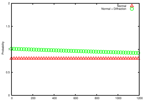
Fig. 5: The total probability integrated over the neutrino angle per time at a finite distance L is given. The constant shows the normal term and the diffraction term is written on top of the normal term. The horizontal axis shows the distance in [m] and the probability of the normal term is normalized to 0.8. Clear uniform excess is seen in the distance below 1200 [m]. The neutrino mass, pion energy, neutrino energy are 0.6 [eV/$c^{2}$], 4 [GeV], and 800 [MeV]. Target is ¹⁶O.

4.2.2 Position dependence

The position dependence of the total probability per time $P/\text{T}$, Eq. $(\ref{total-probability-energy})$ is presented next. $\tilde{g}(\text{T},\omega_{\nu})$ varies with the distance L defined by $\text{L}=c\text{T}$, whereas $G_{0}$ is constant. The probability depends upon the magnitude $\omega_{\nu}\text{T}$ and for the neutrino mass $m_{\nu}=1.0\,[\text{eV}/c^{2}]$ and the pion energy $4$ [GeV] and $4.5$ [GeV] are given in Fig. 4, and for the smaller neutrino mass $m_{\nu}=0.6\,[\text{eV}/c^{2}]$ is given in Fig. 5. $\tilde{g}(\text{T},\omega_{\nu})$ of a lighter mass decreases more slowly with the distance than that of $m_{\nu}=1\,[\text{eV}/c^{2}]$. A longer distance is necessary to see a signal if the neutrino mass is even smaller. For the detection of the muon neutrino, the neutrino energy should be larger than the muon mass, hence the experiment of the energy lower than $100$ [MeV] is impossible. For this energy, the electron neutrino is used then. We present the total probability for the lower energies next. The probability for $m_{\nu}=1.0\,[\text{eV}/c^{2}]$ with the energy $100$ [MeV] is given in Fig. 6. The slowly decreasing component of the probability becomes more prominent with lower values. Hence to observe this component, the experiment of the lower neutrino energy is more convenient.

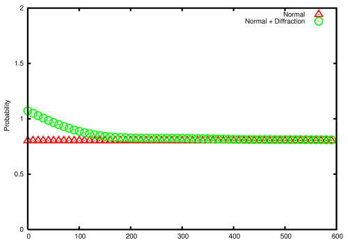
Fig. 6: The total probability integrated over the angle per time at a finite distance L is given. The constant shows the normal term and the diffraction term is written on top of the normal term. The horizontal axis shows the distance in [m] and the probability of the normal term is normalized to 0.8. Clear excess and decreasing behavior are seen in the distance below 600 [m]. The neutrino mass, pion energy, neutrino energy are 1 [eV/$c^{2}$], 4 [GeV], and 100 [MeV]. Target is ¹⁶O.

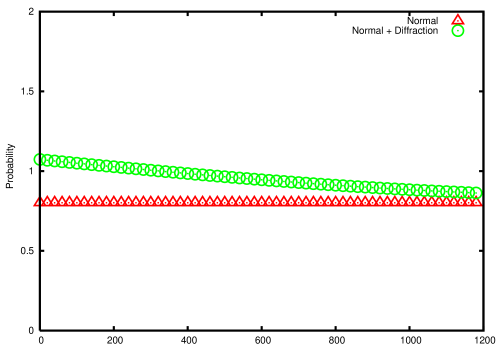
Fig. 7: The probability integrated over the neutrino angle per time at a finite distance L is given. The constant shows the normal term and the diffraction term is written on top of the normal term. The horizontal axis shows the distance in [m] and the probability is normalized to 0.8. Clear excess is seen in the distance below 1200 [m]. The neutrino mass, pion energy, neutrino energy are 0.1 [eV/$c^{2}$], 4 [GeV], and 10 [MeV]. Target is ¹⁶O.

From Eq. $(\ref{probability-31})$, and $\tilde{g}(\text{T},\omega_{\nu})=\frac{c\omega_{\nu}}{2\text{T}}$ at a large T, the typical length $l_{0}$ of the diffraction term is

$$l_{0}~{}[\text{m}]={2E_{\nu}\hbar c\over m_{\nu}^{2}}=400{E_{\nu}[\text{GeV}]\over m_{\nu}^{2}[\text{eV}^{2}/c^{4}]}.$$ (122)

The observation of this component together with the neutrino’s energy would make a determination of the neutrino absolute mass possible. The neutrino’s energy is measured with uncertainty $\Delta E_{\nu}$, which is of the order of $0.1\times E_{\nu}$. This uncertainty is $100$ [MeV] for the energy $1$ [GeV] and is accidentally same order as that of the minimum uncertainty $\hbar/\delta x$ derived from the nuclear size $\delta x$. The total probability for a larger value of energy uncertainty is easily computed using Eq. (118). Figs. 4-7 show the distance dependence of the probability. If the mass is around $1\,[\text{eV}/c^{2}]$ the excess of the neutrino flux of about $20$ percent at the distance less than a few hundred meters is found. We use mainly $m_{\nu}=1\,[\text{eV}/c^{2}]$ throughout this section. Because the probability has a constant term and the T-dependent term, the T-dependent term is extracted easily by subtracting the constant term from the total probability. The slowly decreasing component decreases with the scale determined by the neutrino’s mass and the energy.

We plot the figure for $m_{\nu}=0.1\,[\text{eV}/c^{2}]$, $E_{\nu}=10\,[\text{MeV}]$ in Fig. 7. A decreasing behavior is clearly seen. So in order to observe the slowly decreasing behavior for the small neutrino mass less than or about the same as $0.1\,[\text{eV}/c^{2}]$, the electron neutrino should be used. The decay of the muon and others will be studied in a forthcoming paper.

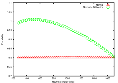
Fig. 8: The energy dependence of the probability integrated over the angle at distance $\text{L}=100$ [m] is given. The lower curve shows the normal term and the diffraction term is added on top of the normal term. The horizontal axis shows the neutrino energy in [MeV] and the probability of the normal term is normalized to 0.8. The neutrino mass and pion energy are 1.0 [eV/$c^{2}$] and 4 [GeV]. Target is ¹⁶O.

4.2.3 Energy dependence

The energy spectrum of the neutrino from the high-energy pion is studied next. Since the diffraction term has the origin in the final states that do not conserve the kinetic energy, that should show unusual behavior. In Fig. 8, the spectrum for the neutrino mass and pion energy, 1.0 [eV/$c^{2}$] and 4 [GeV], are given. The spectrum of the normal term is flat because the energy in the rest system is fixed to one value from the energy-momentum conservation, whereas that of the diffraction is not fixed to one value at the rest system and is not flat but has a maximum at the energy $E_{\nu}\approx{E_{\nu,max}/3}$. The diffraction term becomes much larger in much higher energy.

A unique property of the neutrino diffraction is identified by its energy spectrum.

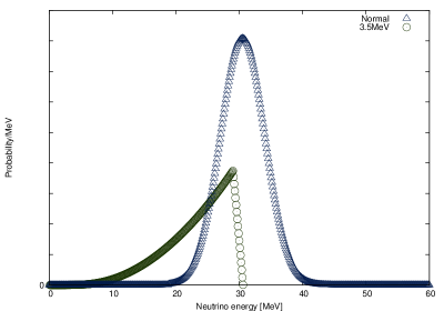
Fig. 9: The neutrino energy spectrum of the normal and diffraction terms in the rest system of the pion are given for the wave packet size of $5$ [MeV]. The former spectrum becomes wide due to the wave packet effect and the latter spectrum becomes wider than the normal component and is in the lower energy region. The magnitude of the diffraction term is arbitrary. The neutrino mass is 1.0 [eV/$c^{2}$]. The length is $\text{L}=10$ [m].

The energy spectrum of the normal term from a pion at rest for the wave packet size of the momentum width $5$ [MeV] is given in Fig. 9. The spectrum has a peak at the value derived from the energy-momentum conservation,

$$m_{\pi}=E_{\nu}+E_{\mu},\ {\vec{p}}_{\nu}+{\vec{p}}_{\mu}=0,$$ (123)

of the two body decay. The neutrino energy is uniquely determined to the value

$$E_{\nu}={m_{\pi}^{2}-m_{\mu}^{2}\over 2m_{\pi}}.$$ (124)

The spectrum becomes broad due to the finite wave packet effect.

The same figure shows another component in the low energy region, which corresponds to the diffraction term. In the low energy region of the neutrino, the light-cone singularity is not dominant and next to leading terms contribute. This figure does not include these non-leading terms, hence the magnitude of the diffraction term is arbitrary. The length is $\text{L}=10$ [m].

Fig. 10 shows the energy spectrum of the fraction of the diffraction term over the normal term, which are computed with the $(V-A)\times(V-A)$ current interaction and is represented in a latter section(Sec.7.3) for ⁵⁶Fe. Its energy is different from Eq. $(\ref{energy-rest})$ and spreads over in a wide energy regions. Only the leading term is taken into account in this figure. Because the energy is away from the normal term, this component may look like a background noise which is uncorrelated with the system. The magnitude becomes small in a lower energy region, because the neutrino spreads uniformly in all angle there. It is noted that the finite-size correction is not invariant under the Lorentz transformation and the magnitude of the diffraction term becomes larger in higher energy.

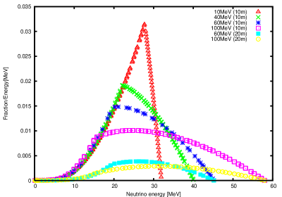
Fig. 10: The neutrino energy spectrum of the fraction of the diffraction term are given for the energy of the pion 10, 40, 100 [MeV/c] and the length $\text{L}=10$ [m], and for the energy of the pion 60, 100 [MeV/c] and the length $\text{L}=20$ [m]. Target is ⁵⁶Fe. The fraction is small in lower energy and is larger in higher energy. The diffraction term may be observable in these energy regions too. The neutrino mass is 1.0 [eV/$c^{2}$].

Thus the fraction of the electron mode varies with the pion’s energy. This unusual behavior is a characteristic feature of the diffraction component. Our result, in fact, shows that this background becomes larger as the pion’s energy becomes larger but has the universal property.

4.2.4 Wide distribution of pion momentum

When a momentum distribution $\rho_{exp}({\vec{p}}_{\pi})$ of initial pions is known, an energy-dependent probability is computed using the expression Eq. $(\ref{total-probability-energy})$. Eq. $(\ref{total-probability-energy})$ is also independent of the position ${\vec{X}}_{\pi}$ and depends upon a pion momentum and a neutrino momentum and the time interval $\text{T}=\text{T}_{\nu}-\text{T}_{\pi}$. In experiments, a position of a pion is not measured and an average over a position is made. An average probability agrees with Eq. $(\ref{total-probability-energy})$. This probability varies slowly with the pion’s momentum and is regarded constant in the energy range of the order of $100$ [MeV]. So the experimental observation of the diffraction term is quite easy.

4.3 On the universality of the diffraction term

The finite-size correction of the probability to detect the neutrino has various unique properties. This component is decreasing with the time interval T, hence the total probability is not proportional to T in this region. In classical particle’s decay, the decay process occurs randomly and follow Markov process. Hence an average number of decay products is necessary proportional to T. Now due to the finite-size correction, this property does not hold. This is not surprising in the interference region $\text{L}\leq l_{0}$, because the quantum mechanical interference effect modifies the probability.

The finite-size correction is expressed with the universal function $\tilde{g}(\omega_{\nu},\text{T})$, where $\omega_{\nu}={m_{\nu}^{2}\over 2E_{\nu}}$. This is determined only with the mass and energy of the neutrino and is independent of details of other parameters of the system such as the size, shape, and position of the wave packets and others. Hence the diffraction component has the genuine property of the wave function $|\text{muon,~{}neutrino}(t)\rangle$, of Eq. $(\ref{state-vector})$, and is capable of experimental measurements.

4.3.1 Violation of conservation laws

The probability is computed with $S[\text{T}]$ and reflects the wave function at a finite time $t$, hence the states of non-conserving kinetic energy contribute to the finite-size correction. So conservation laws that are connected with the space-time symmetry get modified and various probabilities become different from those of $\text{T}\rightarrow\infty$. The leading finite-size corrections have, nevertheless, universal forms that are proportional to $\tilde{g}(\omega,\text{T})$.

4.3.2 Comparisons on the neutrino diffraction with diffraction of classical waves through a hole

1 Inelastic channel.

The neutrino diffraction is the quantum mechanical phenomenon. The neutrino produced in the weak decay of the pion is expressed with the many-body wave function composed of the pion, muon, and neutrino. Hence the probability to detect the neutrino is computed with this many-body wave function. Since this neutrino inside the coherence length is very different from the free isolated neutrino, its probability receives the large finite-size correction of the universal behavior. Its magnitude, however, depends on the wave packet size which is determined with the nucleus that the neutrino interacts with. So the finite-size correction is determined by the many-body wave function and the out-going wave. We should note that quantum mechanical probability is determined with the overlap of the in-coming state with the out-going state and depends on the both states.

In a classical wave phenomenon, on the other hand, an intensity is determined with only the in-coming wave. A magnitude of the in-coming wave is directly observed. Hence the finite-size correction and the interference pattern are determined only by the in-coming wave. Thus interference of the quantum mechanical wave is different from that of the classical wave.
2 Pattern in longitudinal direction

The neutrino diffraction is a part of the finite-size correction that results from the wave natures of the wave function at a finite time $t$. They are generated by the states that are orthogonal to the states at $t\rightarrow\infty$ hence its magnitude is positive semi-definite and depends on the time interval T. Hence the neutrino flux has the excess that decreases with the distance in the direction to the neutrino momentum and vanishes at the infinite distance.

The diffraction pattern of light through a hole or the interference pattern of light in a double slit experiment are different. The intensity have modulations in the perpendicular direction to the wave vector. The interference term is a product of two waves of different phases and so oscillates. Integrating the intensity over the whole screen, the oscillating interference terms cancel and the total intensity is constant.

Thus the diffraction pattern of the neutrino is very different from that of light.
3 $\omega_{\nu}$ is Einstein minus de Broglie frequencies

The pattern of the neutrino diffraction is determined with the angular velocity $\omega_{\nu,diff}=\omega_{\nu,E}-\omega_{\nu,dB}$. Since $\omega_{\nu,E}$ and $\omega_{\nu,dB}$ are almost the same for the neutrino, they are almost cancelled and $\omega_{\nu,diff}$ becomes extremely small and stable in $E_{\nu}$.

The interference pattern of the light on the screen of the double slit experiment, on the other hand, is determined with the angular velocity $\omega_{\gamma,dB}$. Since $\omega_{\gamma,dB}$ is large and proportional to the energy, the pattern varies rapidly with the position in the screen and with the energy. The diffraction pattern of the light passing through the hole varies rapidly.

4.3.3 Muon in the pion decay

In experiments of observing the muon in the pion decays, the neutrino is not observed. In this situation, the muon’s diffraction term has a magnitude that is determined by the ratio of the mass and energy, ${m_{\mu}^{2}/(2E_{\mu})}$.

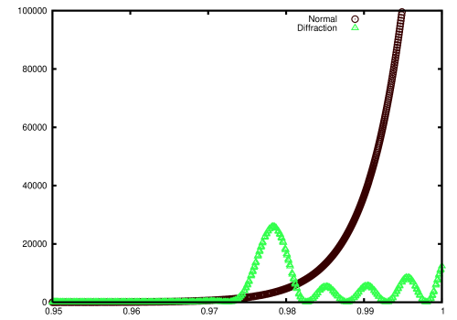
Fig. 11: The angle dependence of the diffraction and normal components of probability is given. The large peak shows the normal component and the small peaks at the tail of the previous peak show the diffraction component. The horizontal axis shows the cosine of the angle between ${\vec{p}}_{\nu}$ and ${\vec{p}}_{\pi}-{\vec{p}}_{\mu}$ and the vertical axis shows the probability. The pion energy, muon energy, and time interval are 250 $m_{\nu}$, 210 $m_{\nu}$, and 30 $m_{\nu}^{-1}$.

Since the muon mass is larger than the neutrino mass by $10^{8}$, the value $m_{\mu}^{2}/(2E_{\mu})$ for the muon is much larger than that of the neutrino by $10^{16}$. For the muon of energy 1 $[\text{GeV}]$, the length is of the order of $l_{0}=10^{-14}$ [m]. This value is a microscopic size and $\tilde{g}(\text{T},\omega_{\mu})$ vanishes at a macroscopic length. Hence the probability of detecting the muon at the macroscopic distance becomes constant. The muon from the pion decay shows neither the finite-size correction nor the diffraction effect. This probability agrees with the production probability. The muon and neutrino behave differently at the finite distance.

If the muon is observed under a condition that the neutrino is detected at the finite T, $S[{\text{T}}]$ is applied and the probability to detect the muon has the contribution from the neutrino diffraction. The diffraction component gives a wide energy spectrum for the muon since that comes from the tail of the distribution function. Fig. 11 shows a probability integrated over the neutrino energy in this condition that both the muon and neutrino are detected, which is obtained from Eq. $(\ref{integrated-amplitude-honbun})$. In this figure, we use units $c=1,\hbar=1$ and express the energy and time with the neutrino mass $m_{\nu}$. Energy of the pion is $250$ $m_{\nu}$ and the muon has the energy $210$ $m_{\nu}$ and has an angle with the pion of $\cos\theta=0.95-1$. The cosine of the angle between ${\vec{p}}_{\pi}-{\vec{p}}_{\mu}$ and ${\vec{p}}_{\nu}$ is in the horizontal axis. T is $30$ $m_{\nu}^{-1}$. The neutrino mass of an unphysical magnitude of the order of MeV and the value of T are chosen in such manner that the numerical computation of diffraction component is easily made. Qualitative features of Fig. 11 are that there exist a large peak at $\cos\theta\approx 1$ and small peaks at the tail region. The former is the peak from the root of $\omega=0$ at $\delta{\vec{p}}\approx 0$ and $\delta E=0$ and the latter are the peaks from the roots of $\omega=0$ of $\delta{\vec{p}}\neq 0$ and $\delta E\neq 0$. The latter peaks, which do not exist in the probability of detecting only the muon, show the feature of the diffraction component of the probability when the neutrino is detected. Thus the diffraction component is observed in the muon also when the neutrino is detected simultaneously. Experimental verification of the diffraction term of this situation using the muon may be made in future.

As was shown in Section 3, the production rate is common to the muon and neutrino, since they are produced in the same decay process. However the rates measured by apparatus depend on the condition of the measurement. If one particle is measured and other is un-measured, its rate for the neutrino receives the large finite-size correction, but the rate for the muon receives no correction. Hence they become different each other. If both particles are measured simultaneously, the rates for both are the same.

Thus the neutrino is in the non-asymptotic region of the finite correlation in wide area, and the transition amplitude for a neutrino that is observed at a finite distance by a nucleus becomes different from that of the infinite distance. The neutrino wave is a superposition of those waves that are produced at different positions and the probability gets an additional contribution and the probability is modified by the diffraction term. The overlap between the neutrino wave that is detected with a nucleus in a detector and those that are produced from a pion decay shows the neutrino diffraction of unique properties. So the neutrino flux measured with its collisions with a nucleus in targets are different from that defined from the norm of wave function.

5 Implications

In this section, various physical quantities of neutrino processes which are modified by the neutrino diffraction are studied. Particularly neutrino nucleon total cross sections, quasi-elastic cross sections, electron-neutrino production anomaly, a proton target enhancement, and an anomaly in atmospheric neutrino are such processes that have significant contributions from the neutrino diffraction.

5.1 Total cross sections of $\nu_{\mu}$-N scattering

Neutrino collisions with hadrons in high energy regions are understood well with the quark-parton model. A total cross section of a high energy neutrino is proportional to the energy and is written in the form

$$\sigma^{\nu}={M_{N}E_{\nu}G_{F}^{2}\over\pi}(Q+1/3\bar{Q}),$$ (125)

using integrals of quark-parton distribution functions $q(x)$ and $\bar{q}(x)$ and $Q=\int_{0}^{1}dxxq(x),\bar{Q}=\int_{0}^{1}dxx\bar{q}(x)$. The cross section is proportional to the neutrino energy and a current value is $\sigma_{\nu}/E=0.67\times 10^{-38}[\text{cm}^{2}/\text{GeV}]$.

Now the rate of process of the neutrino produced by a decay of a pion and interacting with a nucleus has a finite-size correction. It modifies the probability of the neutrino collision and the cross section. We estimate its effect hereafter. Including the diffraction term, the effective neutrino flux becomes the sum of the normal and diffraction terms

$$f=f_{normal}(1+r_{diff}),$$ (126)

where $r_{diff}$ is the rate of the diffraction component over the normal component, and is a function of the combination $({m_{\nu}^{2}\over 2cE_{\nu}}\text{L})$,

$$r_{diff}=d_{0}\tilde{g}(\frac{m_{\nu}^{2}}{2cE_{\nu}}\text{L}),$$ (127)

where L is a length of the decay volume and the coefficient $d_{0}$ is determined from geometries of experiments.

When a detector is located at the end of the decay volume, the correction factor Eq. $(\ref{E-depedent-correction})$ is used. In actual case, the detector is located in a distant region from the decay volume. There are material or soil between them and pions are stopped in beam dump. The neutrino is produced in the decay region and propagates freely afterward. Since the wave packets of one $\sigma_{\nu}$ form the complete set [10], the wave packet of the size at the decay volume is the $\sigma_{\nu}$ determined with the detector. The neutrino flux at the end of the decay volume is computed with the diffraction term of the decay volume ’s length L and the wave packet size of the detector. Wave packets of this $\sigma_{\nu}$ propagate freely from the end of decay volume to the detector. The final value of neutrino flux at the detector is found combining both effects. When neutrino changes flavor in this period, the final probability for each flavor is written with a usual formula of flavor oscillation.

The true neutrino events in experiment is converted to the cross section, $\sigma^{exp}(E)$, that includes the diffraction component and is connected with the cross section computed with only the normal component $\sigma^{the}(E)$ by the rate

$$\sigma^{the}(E)=\sigma^{exp}(E){1\over 1+r_{diff}}.$$

Conversely the experimental cross section is written as

$$\sigma^{exp}(E)/E=(1+r_{diff})(\sigma^{the}(E)/E).$$ (128)

$\sigma^{the}(E)/E$ is constant from Eq. (125) so the E-dependence of $\sigma(E)^{exp}/E$ is due to E-dependence of $r_{diff}$, Eq. $(\ref{E-depedent-correction})$.

The correction $r_{diff}$ depends on the geometry of experiments and the material of the detector. We compute $r_{diff}$ using the experimental conditions of MINOS [30] and NOMAD [31] and the total cross sections.

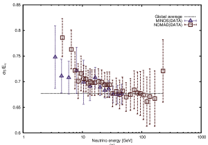
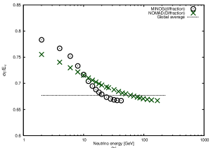
Fig. 12: Neutrino-Nucleon total cross section of MINOS and NOMAD (a) and total cross sections of the sums of normal and diffraction terms in geometries of MINOS and NOMAD (b) are given. The horizontal axis shows the neutrino energies in [GeV] and the vertical axis shows the ratio of the cross section over the energy.

The geometry of MINOS and NOMAD are the following. The lengths between the pion source and the neutrino detector, $\text{L}_{det-so}$, and those of the decay region, $\text{L}_{decay-reg}$, are:

$$NOMAD~{} : \text{L}_{det-so}=835\,[\text{m}],\ \text{L}_{decay-reg}=290\,[\text{m}],$$ (129)

$$MINOS~{} : \text{L}_{det-so}=1040\,[\text{m}],\ \text{L}_{decay-reg}=675\,[\text{m}].$$ (130)

Also pion beam spreading was included from angle of initial pion; $0$ to $10\,[\text{mrad}]$ for NOMAD and $0$ to $15\,[\text{mrad}]$ for MINOS.

The wave packet size is estimated with the size of target nucleus. From the size of the nucleus of the mass number $A$, we have $\sigma_{\nu}=A^{\frac{2}{3}}/m_{\pi}^{2}$. For various material the value are

$$\sigma_{\nu}=5.2/m_{\pi}^{2};{}^{12}C~{}nucleus.$$

$$\sigma_{\nu}=14.6/m_{\pi}^{2};{}^{56}Fe~{}nucleus.$$ (131)

Including the geometries, beam spreadings, and wave packet sizes, we computed the total cross sections and compared with the experiments in Fig. 12. These cross sections computed theoretically slowly decrease with the energy in the geometry dependent manner and agree with the experiments. Since the experimental parameters such as the neutrino energy and others are different in two experiments, the agreements of the theory with the experiments are highly non-trivial. So the large cross sections at low energy regions may be attributed to the diffraction component.

We have compared only NOMAD and MINOS here. Many experiments are listed in particle data [32] and most of them have similar energy dependences and agree qualitatively with the presence of the diffraction components. It is important to notice that the magnitude of diffraction component is sensitive to geometry. Furthermore if a kinematical constraint Eq. (110) on the angle between ${\vec{p}}_{\pi}$ and ${\vec{p}}_{\nu}$ was required, only the events of the normal term was selected. Then the cross section should agree with that of the normal term.

5.2 Quasi-elastic cross sections

Quasi-elastic or one pion production processes are understood relatively well theoretically. The diffraction modifies the total events of these processes also.

The cross sections for

$$\nu+n\rightarrow\mu^{-}+p(+\pi^{0}),$$ (132)

$$\nu+p\rightarrow\mu^{-}+p+\pi^{+},$$ (133)

$$\bar{\nu}+p\rightarrow\mu^{+}+n(+\pi^{0}),$$ (134)

and the neutral current process

$$\nu+N\rightarrow\nu+N(+\pi^{0}),$$ (135)

are known well using CVC, PCAC, and vector dominance and are studied recently by MiniBooNE [33]. The parameter is the axial vector meson $M_{A}$ and higher mass contributions. So these cross section are used to study the diffraction terms.

5.3 Electron neutrino anomaly

In pion decays, a branching ratio of an electron mode is smaller than that of a muon mode by factor $10^{-4}$ due to the helicity suppression of the decay of a pseudo-scalar particle caused by the charged current interaction. This behavior of the total rates has been confirmed by the observations of charged leptons.

Now the probability to detect a neutrino inside the coherence length, where the neutrino retains the wave natures, is affected by the finite-size correction. Because this correction comes from the states that have different kinetic-energy from the initial value, the neutrino in this region does not follow the conservation law satisfied in the asymptotic region $t\rightarrow\infty$. The rate that electron neutrino is detected is not suppressed. The ratio of the probability to detect the electron neutrino over that of the muon neutrino becomes substantially larger in near-detector regions.

To compute the transition probability and the spectra of electron and muon neutrinos, we start from the $(V-A)\times(V-A)$ interaction Lagrangian (Hamiltonian). The result of the probability is almost the same as that of Eq. $(\ref{weak-hamiltonian})$ in the muon mode but is different in the electron mode since the diffraction component does not satisfy the rigorous conservation of the kinetic-energy and momentum. In I, it was found that the initial pion is described by a wave packet of a large size. Hence the initial pion of the plane wave is studied here. The amplitude $T$ is written with the hadronic $V-A$ current and Dirac spinors in the form

$$T=\int d^{4}xd{\vec{k}}_{\nu}\,N\langle 0|J_{V-A}^{\mu}(x)|\pi\rangle\bar{u}({\vec{p}}_{l})\gamma_{\mu}(1-\gamma_{5})\nu({\vec{k}}_{\nu})$$

$$\times e^{ip_{l}\cdot x+ik_{\nu}\cdot(x-\text{X}_{\nu})-\frac{\sigma_{\nu}}{2}({\vec{k}}_{\nu}-{\vec{p}}_{\nu})^{2}},$$ (136)

where $N=ig\left({\sigma_{\nu}/\pi}\right)^{\frac{4}{3}}\left({m_{l}m_{\nu}}/{E_{l}E_{\nu}}\right)^{\frac{1}{2}}$, and the time $t$ is integrated in the region $\text{T}_{\pi}\leq t\leq\text{T}_{\nu}$. The transition probability to this final state is written, after the spin summations are made, with the correlation function and the neutrino wave function in the form

$$\int\frac{d{\vec{p}}_{l}}{(2\pi)^{3}}\sum_{s_{1},s_{2}}|T|^{2}=\frac{C}{E_{\nu}}\int d^{4}x_{1}d^{4}x_{2}e^{-\frac{1}{2\sigma_{\nu}}\sum_{i}({\vec{x}}_{i}-\vec{x}_{i}^{\,0})^{2}}\Delta_{\pi,l}(\delta x)e^{i\phi(\delta x)},$$ (137)

where $C=g^{2}\left({4\pi}/{\sigma_{\nu}}\right)^{\frac{3}{2}}V^{-1}$, $V$ is a normalization volume for the initial pion, $\vec{x}_{i}^{\,0}=\vec{\text{X}}_{\nu}+{\vec{v}}_{\nu}(t_{i}-\text{T}_{\nu})$, $\delta x=x_{1}-x_{2}$, $\phi(\delta x)=p_{\nu}\!\cdot\!\delta x$ and

$$\Delta_{\pi,l}(\delta x)={\frac{1}{(2\pi)^{3}}}\int\frac{d{\vec{p}}_{l}}{E({\vec{p}}_{l})}\left(2(p_{\pi}\cdot p_{\nu})(p_{\pi}\cdot p_{l})-m_{\pi}^{2}(p_{l}\cdot p_{\nu})\right)e^{-i(p_{\pi}-p_{l})\cdot\delta x}.$$ (138)

The probability of detecting a neutrino of $p_{\nu}$ at ${\vec{X}}_{\nu}$ and a lepton $l$ of arbitrary momentum is expressed as the sum of the normal term $G_{0}$ and the diffraction term $\tilde{g}(\text{T},\omega_{\nu})$,

$$P=N_{2}\int\frac{d^{3}p_{\nu}}{(2\pi)^{3}}\frac{p_{\pi}\!\cdot\!p_{\nu}(m_{\pi}^{2}-2p_{\pi}\!\cdot\!p_{\nu})}{E_{\nu}}\left[\tilde{g}(\text{T},\omega_{\nu})+G_{0}\right],$$ (139)

where $N_{2}=8\text{T}g^{2}\sigma_{\nu}$ and $\text{L}=c\text{T}$ is the length of decay region. In $G_{0}$ the energy and momentum are conserved approximately well and

$$p_{l}\approx p_{\pi}-p_{\nu},$$ (140)

is satisfied. Hence from a square of the both hand sides, the mass shell condition

$$m_{l}^{2}\approx m_{\pi}^{2}-2p_{\pi}\cdot p_{\nu},$$ (141)

is obtained. Thus the normal terms are proportional to the square of lepton masses and the electron mode is suppressed [4, 5, 6, 9]. In $\tilde{g}(\text{T},\omega_{\nu})$, on the other hand, momenta satisfy

$$p_{l}\neq p_{\pi}-p_{\nu},$$ (142)

and the diffraction terms are not proportional to the square of lepton masses and the electron mode is not suppressed.

The total probability of detecting a neutrino or a charged lepton in the pion decay at macroscopic distance is written in the form,

$$P=P_{normal}+P_{diff}^{l}.$$ (143)

In Eq. $(\ref{probability-lepton})$, $P_{normal}$ is the normal term that is obtained from the decay probability $G_{0}$ in Eq. $(\ref{probability-leptons})$ and $P_{diff}^{l}$ is the diffraction term that is determined from $\tilde{g}$ in Eq. $(\ref{probability-leptons})$. The former probability agrees to that obtained using the plane waves and the latter one has not been included before and its effect is estimated here. The diffraction term at T is described with its mass and energy in the universal form

$$P_{diff}^{l}=C\text{T}\tilde{g}(\text{T},\omega_{l}).$$ (144)

The frequency $\omega_{l}$ are small for neutrinos and large in charged leptons. $\tilde{g}(\text{T},\omega_{l})$ is positive definite and decreases slowly with a distance L and vanishes at infinite distance. Hence at $\text{L}=\infty$, the probability agrees with the normal component,

$$P=P_{normal}.$$ (145)

The length scale ${2cE_{l}/m_{l}^{2}}$ is macroscopic size in neutrinos but is $10^{-10}$ [m] or less for the electron and muon. The magnitude of $\tilde{g}(\text{T},\omega_{l})$ at the macroscopic distance is given in Fig. 2 of I. At $\text{L}=100\,[\text{m}]$, $E=1\,[\text{GeV}]$ for the mass $1\,[\text{eV}/{c^{2}}]\,(\nu)$, $0.5\,[\text{MeV}/{c^{2}}]\,(e)$, and $100\,[\text{MeV}/{c^{2}}]\,(\mu)$, the values are,

$$\tilde{g}(\text{T},\omega_{\nu})\approx 3,$$

$$\tilde{g}(\text{T},\omega_{e})\approx 0,$$

$$\tilde{g}(\text{T},\omega_{\mu})\approx 0.$$ (146)

In this region, they satisfy

$$\tilde{g}(\text{T},\omega_{l})\approx{m_{\nu}^{2}\over m_{l}^{2}}\tilde{g}(\text{T},\omega_{\nu}),$$ (147)

hence the diffraction component at a macroscopic distance is finite in the neutrino and vanishes in others. It is striking that the probability to detect the neutrino has an additional term and is not equivalent to that of the charged lepton even though they are produced in the same decay process.

The diffraction term is generated by the tiny neutrino mass and the light-cone singularity. Hence the pattern is determined by $(E({\vec{p}}_{\nu})-c|\vec{p}_{\nu}|)t$ and becomes long-range. Because $P_{diff}$ is the finite-size correction caused by the neutrino interference, it has different properties from $P_{normal}$ in flavor and momentum dependences. The neutrino diffraction furthermore is sensitive to the absolute neutrino mass. We study implications of the diffraction term to the electron mode in the pion decays here.

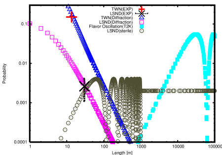
Fig. 13: Experiments of LSND and TWN are compared with the theoretical values of the diffraction terms. TWN(EXP) and LSND(EXP) show the experimental values and TWN(Diffraction) is computed with the parameters $m_{\nu}=0.2\,[\text{eV}/c^{2}]$, $E_{\nu}=250[\text{MeV}]$, $P_{\pi}=2[\text{GeV}/c]$, LSND(Diffraction) is computed with $m_{\nu}=0.2\,[\text{eV}/c^{2}]$, $E_{\nu}=60\,[\text{MeV}]$, $P_{\pi}=300\,[\text{MeV}/c]$. Flavor oscillation oscillation(T2K) shows the values for $\sin^{2}\theta_{13}=0.11$, $\delta m^{2}_{23}=2.4\times 10^{-3}\,[\text{eV}^{2}/c^{4}]$, $E_{\nu}=60\,[\text{MeV}]$, and LSND(sterile) shows with $\sin^{2}\theta=0.004$, $\delta m^{2}=1.2\,[\text{eV}^{2}/c^{4}]$, $E_{\nu}=60\,[\text{MeV}]$.

In Fig. 13, experiments of LSND [34] and the two neutrino experiment( TWN) [35] are compared with the diffraction components and the flavor oscillations. Theoretical values are obtained including geometries of the experiments. Since those of LSND and TWN are different, the theoretical value for the LSND are smaller than that for TWN. The experimental values plotted with crosses agree with the theoretical values. The values from the flavor oscillations expected from the current parameters are also shown. The mass-squared differences and mixing angles from the recent ground experiments lead negligible values for both experiments. A sterile neutrino of the mass around $1$ $[{\text{eV}}/c^{2}]$ is necessary to fit the data of LSND with the flavor oscillation. The agreements of the values from the neutrino diffraction in LSND and TWN suggest that it is unnecessary to introduce additional parameters.

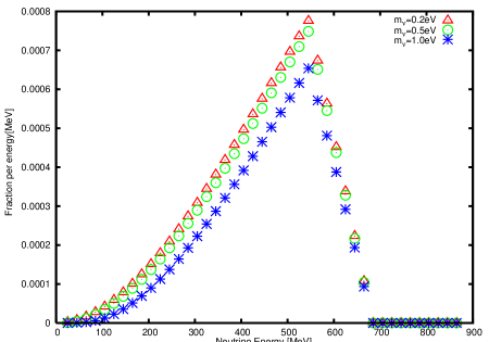
Fig. 14: Fraction of the electron neutrino of the mass 0.2 $[\text{eV}/c^{2}]$, 0.5 $[\text{eV}/c^{2}]$ and 1$[\text{eV}/c^{2}]$ at L=110 [m], distance=170 [m] of T2K geometry and $P_{\pi}=2$ [GeV/$c$].

In Fig. 14, the maximum possible fraction of the electron neutrino in a geometry of T2K experiment is shown. The spreading of the pion beam is ignored in this Figure. Since the diffraction is sensitive to the pion beam spreading, the real value may becomes smaller than this figure.

5.4 Proton target anomaly

Magnitude of diffraction component depends upon the size of the nucleus which neutrino interacts with and is expressed by the wave packet size $\sigma_{\nu}$. It becomes larger with the larger target. It is known and used in the text that nuclear size is proportional to $A^{\frac{2}{3}}$ and the large $A$ nuclear gives a large diffraction component, generally. Proton has a smallest intrinsic size. However a proton is expressed by a wave function of its position in matter. So the wave packet size is determined by a size of this wave function. Since a proton is the lightest nucleus, it has the largest size. We estimate this size using center of mass gravity effect between proton and electron. For the proton’s mass $m_{p}$ and the electron mass $m_{e}$, an electron’s coordinate ${\vec{x}}_{electron}$ and the proton coordinate ${\vec{x}}_{p}$ are expressed as,

$${\vec{x}}_{electron}={\vec{X}}+{m_{p}\over m_{e}+m_{p}}{\vec{r}}\approx{\vec{X}}+(1+{1\over 2000}){\vec{r}},$$

$${\vec{x}}_{p}={\vec{X}}-{m_{e}\over m_{e}+m_{p}}{\vec{r}}\approx{\vec{X}}-{1\over 2000}{\vec{r}}.$$ (148)

If the wave function of the atom is

$$\Psi({\vec{R}})\varphi({\vec{r}}),$$ (149)

and the function of the relative coordinate, $\varphi({\vec{r}})$, is extended by an amount $R_{atom}$ which is about $10^{-10}[\text{m}]$ then the proton is extended with a radius

$$R_{p}={1\over 2000}R_{atom}\approx 5\times 10^{-14}\,[\text{m}].$$ (150)

This value is much shorter than the atomic scale and is larger than one nucleon’s size $1\,[\text{fm}]=10^{-15}\,[\text{m}]$ by factor $50$. Thus proton in solid is extended to the size ${1\over 2000}$ of the atomic wave function, which is larger than the nuclear size of O. Hence proton gives the important role in the neutrino diffraction. Its size may be in the range

$$l_{proton}(U)=5\times 10^{-14}-10^{-13}\,[\text{m}].$$ (151)

An enhancement of diffraction contribution due to the proton is expected in

$$\bar{\nu}+p\rightarrow\mu^{+}+X^{0},\ X^{0}=n,\ p\pi^{-},\ n\pi^{0},\ others.$$ (152)

5.5 Atmospheric neutrino

The neutrino flavor oscillation was found first with an atmospheric neutrino. Neutrinos are produced from decays of charged pions and muons in secondary cosmic rays. Since the matter density is low in atmosphere, these charged particles travel freely long distance. Thus neutrinos produced in decays of pions or muons show the diffraction phenomenon and the diffraction components are added to the neutrino fluxes. These neutrino events may be observed in detectors set in the ground, such as Super-KamiokaNDE(SK) if the absolute mass is a reasonable value. The minimum mass allowed from the mass-squared difference is about the value, $\sqrt{\delta m^{2}}\approx 10^{-2}\,[\text{eV}/c^{2}]$. Then the length that the diffraction component is observed becomes $\text{L}_{0}={2E_{\nu}c\over m_{\nu}^{2}}\approx 20\,[\text{km}]$ for $E_{\nu}=1\,[\text{GeV}]$, which is longer than the height of troposphere. Hence the diffraction component could be observed with the angle-dependent excess of the electron and muon neutrino fluxes. Since the diffraction components from pion decays are common to both neutrinos, their ratio is not sensitive to the diffraction. Instead of this ratio, a ratio of the neutrino flux to the flux of charged leptons is good to see the signal of the neutrino diffraction.

6 Behaviors of the probability suggest violations at first sight but do not so in fact.

6.1 Unitarity

Probability of detecting the neutrino per time $P(\text{L})$ decreases with the distance L. This behavior of the probability appears to suggest that the probability is not preserved and is inconsistent with the unitarity. However this behavior is derived from the $S[\text{T}]$ that satisfies $S^{\dagger}[\text{T}]S[\text{T}]=1$ and is consistent with the unitarity. The probability at L is determined with S-matrix $S[\text{T}],\ \text{L}=c\text{T}$ and has two components $P=P^{(normal)}+P^{diff}(\text{L})$. Both terms are positive semi-definite and the latter is decreasing with L because the constraint to the final state from the energy conservation becomes more stringent with increasing L. This decreasing behavior is a natural consequence of the unusual properties of the finite-size correction and is consistent with the unitarity $S^{\dagger}[\text{T}]S[\text{T}]=1$. The unitarity leads that the life time of the pion becomes larger if the neutrino is detected at a finite T.

6.2 Lepton number non-conservation

The probability of the pion decay process in the situation where the neutrino is detected has the large finite-size correction. The charged lepton shows the same behavior in the same situation. This will be confirmed if the charged lepton is measured simultaneously with the neutrino in experiments. This has not been done and is consistent with the lepton number conservation.

The probability of the pion decay process in another situation where the neutrino is un-detected has no finite-size correction. The charged lepton in this process does not show the finite-size correction and its decay probability is computed with the standard calculation of using the plane waves. This situation has been studied well experimentally and agrees with the theoretical calculations obtained with $S[\infty]$.

Now the boundary conditions of the above two cases are different. One boundary condition leads uniquely one consequence and the different boundary conditions may lead the different probabilities. Our results show that the different boundary condition on the neutrino leads the different result on the decay probability. Thus the probability to detect the neutrino in the first case is different from that of the charged lepton in the second case. It is meaningless to compare the probability for neutrino in the first case with that for the charged lepton in the second case, because they follow the different boundary conditions.

Since the probability of detecting the neutrino at a finite distance deviates from that at the infinity and the probability of producing the neutrino is defined with the value at the infinite distance, they are different. The fact that the probability of detecting the neutrino is different from that of the charged lepton does not mean the violation of the lepton number conservation, but means that the probabilities depend on the boundary condition. The lepton number is conserved. Thus the different behavior of the probability from that of the production is similar to that of the retarded electric potential of a moving charged body.

6.3 Dependence on wave packet size

It is known that the total probability at $\text{T}=\infty$ does not depend on the wave packet size [24]. The result of the present paper Eq. $(\ref{total-probability-energy})$ in fact shows that the first term in the right-hand side is independent of the wave packet size. Now the second term in Eq. $(\ref{total-probability-energy})$, which is the finite-size correction, is proportional to $\sigma_{\nu}$. Since $S[\text{T}]$ is determined with the wave packets, its boundary conditions are determined with $\sigma_{\nu}$ and the finite-size correction depends on $\sigma_{\nu}$. That increases with $\sigma_{\nu}$ and diverges at $\sigma_{\nu}=\infty$. The diverging correction at $\sigma_{\nu}=\infty$ is consistent, in fact, with the fact that the total cross section diverges for the plane waves [27]. This occurs because the denominator of the neutrino propagator vanishes. Nevertheless the finite-size correction has the universal properties, which were computed with $S[\text{T}]$ defined by the wave packets.

7 Unusual features

7.1 Energy non-conservation and violation of symmetries

The S-matrix at the finite-time interval $S[\text{T}]$ does not commute with the free Hamiltonian $H_{0}$, and satisfies Eq. $(\ref{commutation-relation-S(T) })$. In this region, one pion and decay products co-exist in a coherent manner that is determined by $H_{1}$. Hence $H_{1}$ has a finite expectation value and the kinetic energy defined by the free part $H_{0}$ is different from that of $H$. $H_{0}$ is not conserved in $S[\text{T}]$, despite the fact that the total energy defined by $H$ is conserved. The contribution to the transition probability from these states was computed in the text analytically. They exhibit the neutrino diffraction and give the finite-size correction to the neutrino flux.

The finite-size correction is not invariant under Lorenz transformation either and the magnitude of the diffraction term in the pion rest system is smaller than that in the high energy pion.

7.2 Helicity suppression

Decay rate of the pion to the electron mode is suppressed over that to the muon mode by the helicity suppression. The helicity suppression hold in a decay of a pseudo-scalar particle to a neutrino and lepton caused by $V-A$ weak interaction. Conservations of the kinetic energy and the angular momentum enforce vanishing of the amplitude for the massless lepton. Now the kinetic energy is not conserved in the non-asymptotic region and the helicity suppression is not effective. The probabilities to detect the neutrino in this region are not suppressed. Thus the normal terms hold these properties and the electron mode is suppressed, whereas the finite-size correction does not hold these properties. The electron mode is not suppressed in the diffraction component and has the sizable magnitude in the spatial region where the normal term is negligible.

Thus when the neutrino is observed in near-detector region, the electron neutrino is substantially enhanced.

7.3 Large finite-size correction

The finite-size correction of the probability to detect the neutrino is finite in the spatial region $\text{L}\leq l_{0}$ of the distance L between the pion and the neutrino, where the interaction energy is finite and the energy defined by the free Hamiltonian $H_{0}$ deviates from the conserved total-energy. The states of these energies of $H_{0}$ that are different from that of the initial state interact with $S[\text{T}]$ in a universal manner that is determined by $H_{1}$ and gave the finite-size correction. Particle spectrum at ultra-violet region is universal in relativistic invariant systems and gives the light-cone singularity to correlation functions. The light-cone singularity is real and extended to a large area and gives the universal finite-size correction to light particles. It might be remarkable that the states of the ultraviolet region give the observable effect to the probability of the tree diagram.

Since the probability to detect the neutrino has the large finite-size correction, the neutrino detection affects strongly the pion decay probability. The decay rate of the pion in the situation where the neutrino is detected is different from that where the neutrino is un-detected, because they are described by the amplitude of the different boundary conditions.

The life time of the pion in which the produced neutrino is observed becomes shorter than the normal value. This phenomenon that the life time is modified by its interaction with matters is known in the literature as quantum Zeno effect. Neutrinos actually interact extremely weakly with matters and a majority of neutrinos are passing freely without any interaction and are not affected by this effect. Consequently the majority of the pions are not affected by the finite-size effect and its life time is not modified and has the normal life time. Although the detected neutrino receives the large finite-size correction, its effect is negligibly small for observables of the pions.

7.4 Interference in parallel direction to the momentum

The diffraction term depends on the time interval T and is positive definite. Its pattern changes with the distance L extremely slowly. Thus the interference pattern is along the parallel direction to the momentum.

7.5 Dependence on the apparatus

The neutrino diffraction appears in the quantum mechanical transition probability and depends on both the initial and final states. The wave function of the final state is determined by the apparatus and so are the scattering amplitude and probability. It is in fact quite reasonable that the interference pattern depends on the apparatus in quantum mechanics. In classical physics, on the other hand, any physical variables are observable and interference patterns do not depend on the apparatus. Hence the fact that interference pattern of the probability of the present work depends upon the apparatus and is quite different from that of the classical physics is not surprising.

8 Summary and implications

We found that the neutrino in the pion decay has a large non-asymptotic region of having wave natures and the probability to detect the neutrino in this region reveals unusual property. The neutrino is unique and shows the large finite-size correction of the diffraction form. The unusual diffraction pattern is caused by the relativistic invariance and the tiny neutrino mass. Its origin, mechanism, characteristic features, and implications are presented.

The pion, neutrino, and charged lepton are described by a many-body wave function that follows the Schrödinger equation. The wave function at a finite $t$ has various unusual properties that are different from those at $t\rightarrow\infty$. Especially the total kinetic energy is different from that of the initial state and takes a wide range of values. Hence the wave functions of these particles vary in space and time. The physical quantities of these wave functions are computed by the S-matrix at a finite-time interval that satisfies the boundary condition at a finite time. The position-dependent probability to detect neutrino, which is proportional to the flux, was computed with the $S[\text{T}]$ expressed by wave packets and the large finite-size correction of universal property that is insensitive to the pion’s initial conditions was found. The pion’s mean free path estimated in Appendix of I shows that this is long enough for the new term to be observed in the experiments. The diffraction term reflects the finite-size correction, and depends on the distance, energy, angle, and the absolute neutrino mass in the universal manner.

The wave function at a finite $t$ has the continuous kinetic energy that leads the space-time dependent wave nature, which is probed with the wave packet localized in space. Eq. $(\ref{integrated-amplitude-honbun})$ is derived in this manner and shows a reason why the probability has the large finite-size correction. The angular velocity $\omega$ is given by the energy of the moving frame $\omega=\delta E-{\vec{v}}_{\nu}\cdot\delta{\vec{p}}$, consequently $\omega=0$ has the root of $\delta E\neq 0$ and $\delta{\vec{p}}\neq 0$ in addition to that of $\delta E=0$ and $\delta{\vec{p}}=0$. The former root exists only in $S[\text{T}]$ and gives the finite-size correction. The probability around the former root receives also the finite-size correction, as is shown also in Appendix B. Since the kinetic energy and momentum are not conserved in this root, the finite-size correction has various unusual properties. Thus the states which violate the energy and momentum conservation give the correction. To compute the dominant contribution in the long-distance region rigorously, it is convenient to interchange the order of the integrations and introduce the correlation function $\Delta_{\pi,\mu}({\delta x})$. The states of non-conserving the energy and momentum form the light-cone singularity of $\Delta_{\pi,\mu}({\delta x})$ and give the most important contribution to the finite-size correction of the probability to detect the neutrino. The regular terms of $\Delta_{\pi,\mu}({\delta x})$ give the constant value of the probability.

The light-cone singularity is formed from the superposition of waves of the infinite momentum, which have always the light velocity and vanishing complex phase. So when it is combined with the slow phase $\bar{\phi}_{c}$ of the neutrino wave function, Eq. $(\ref{light-phase})$, this slow phase remains to physical observable.

The slow phase of the neutrino wave packet is the outcome of the cancellation between the time and space parts of extremely light neutrino. The phase is determined by the difference of space-time coordinates $(\delta t,\delta{\vec{x}})$ and the central values of the energy and momentum, as ${E({\vec{p}}\,)\delta t-{\vec{p}}\!\cdot\!\delta{\vec{x}}}$, where the energy $E({\vec{p}}\,)$ is given by $\sqrt{{\vec{p}}^{\,2}+m^{2}}$. When the difference of positions $\delta{\vec{x}}$ is moving with the light velocity in the parallel direction to the momentum ${\vec{p}}$, ${\vec{v}}_{c}=c({\vec{p}}/|\vec{p}|)$, as $\delta{\vec{x}}={\vec{v}}_{c}\delta t$, then the total phase becomes $E_{\nu}\delta t-{\vec{p}}_{\nu}\!\cdot\!\delta{\vec{x}}=(m_{\nu}^{2}/2E_{\nu})\delta t$. The angular velocity becomes the small value $m_{\nu}^{2}/(2E_{\nu})$ and makes the interference phenomenon long-range. The new term in the probability decreases slowly with the distance in the universal manner determined by the mass and energy of the neutrino as $m_{\nu}^{2}/(2E_{\nu})$. This form is independent from the details of wave packet shape and parameters as far as the reality of the neutrino wave function $\tilde{w}({\vec{x}})$ is satisfied, which is ensured from the invariance under the time inversion. The relative magnitude of this component is not universal and depends upon the size of wave packet. Based on the estimation of the size, we found that the magnitude of the new universal term is sizable for the measurement. Since the slope of the diffraction component is determined by the mass and energy of the neutrino, the absolute value of the neutrino mass would be found from the neutrino interference experiments.

The diffraction components were compared with several previous neutrino experiments in Section 7. First, the slight energy dependence of the total neutrino-nucleon cross sections at high energy regions, which is hard to understand in the standard theory, was shown to agree with the excess of the effective neutrino flux due to the diffraction. The excesses of neutrino events will be observed in other reactions as well at macroscopic short distance regions. Theoretical calculations at distances of the order of a few hundred meters were computed and shown in Figures of Section 6. From these figures, the excesses are not large but are sizable magnitudes. Hence these excesses shall be observed in these distances. Actually fluxes measured in the near detectors of the long-baseline experiments of K2K [36] and MiniBooNE [37] may show excesses of about $10-20$ percent of the Monte Carlo estimations. Monte Carlo estimations of the fluxes are obtained using naive decay probabilities and do not have the coherence effects we presented in the present work. So the excess of these experiments may be related with the excesses due to interferences. The excess is not clear in MINOS [38]. With more statistics, qualitative analysis might become possible to test the new universal term on the neutrino flux at the finite distance. If the mass is in the range from $0.1\,[\text{eV}/c^{2}]$ to $2\,[\text{eV}/c^{2}]$, the near detectors at T2K, MiniBooNE, MINOS and other experiments might be able to measure these signatures.

Second, the suppression of the electron mode in pion decay is modified in the probability to detect neutrinos. Since the energy-momentum conservation does not hold in the $S[\text{T}]$, the helicity suppression mechanism does not work in the diffraction component. So the electron mode is enhanced drastically. The theoretical value of fraction that includes the finite-size correction of the electron mode was compared with LSND and TWN, and agreements were obtained. Further confirmation of the diffraction component by observing the electron neutrino in pion decay will be made using modern version of LSND or similar experiments. T2K near detector is a possible place for that. Third, anomalies in proton target, and atmospheric neutrino would supply also specific signature of the neutrino diffraction. The neutrino diffraction is sensitive to the absolute neutrino mass but is not so to other parameters such as pion and neutrino energies. Hence the observations of the neutrino diffraction is easy. The absolute neutrino mass could be found with these experiments.

At the end, we summarize the reasons why the interference term of the long-distance behavior emerges in the pion decay and is computed with the wave packet representation. The connection of the long-distance interference phenomenon of the neutrino with the Heisenberg’s uncertainty relation is also addressed.

Relativistic invariance forces the particle’s momentum unlimited and makes the correlation function $\Delta_{\pi,\mu}(\delta t,\delta\vec{x})$ have a singularity near $\lambda=0$, which is extended to large distance $|\delta{\vec{x}|}\rightarrow\infty$. This is one of the features of relativistic quantum fields in Minkowski space-time and is one reason why the long-range correlation emerged. For a non-relativistic system, on the other hand, the same calculation for stationary states is made by,

$$\int d{\vec{k}}\langle{\vec{x}}_{1}|{\vec{k}}\rangle\langle{\vec{k}}|{\vec{x}}_{2}\rangle=\delta({\vec{x}}_{1}-{\vec{x}}_{2}),$$ (153)

and the only one point $\delta{\vec{x}}=0$ satisfies the condition. Long-range correlation is not generated. The rotational invariant three-dimensional space is compact but the Lorentz invariant four-dimensional space is non-compact. So it is quite natural for the non-relativistic system not to have the long-range correlation that the relativistic system has. The light-cone singularity is the peculiar property of the relativistic system.

Heisenberg uncertainty relation is slightly modified in the wave along the light cone. The neutrino wave function behaves at large distance along the light-cone region in the form

$$\psi_{\nu}(t,{\vec{x}})=f{e^{i(E_{\nu}t-{\vec{p}}_{\nu}\cdot{\vec{x}})}\over x}=f{e^{i{m_{\nu}^{2}\over 2E_{\nu}}t}\over ct},$$ (154)

where $f$ has no dependence on the distance $|\vec{x}|$. Consequently the uncertainty relation between the energy width $\delta E$ and the time interval $\delta t$ becomes

$$\delta t\delta{m_{\nu}^{2}\over 2E_{\nu}}=\delta t\delta E\times{1\over 2}\left({m_{\nu}\over E_{\nu}}\right)^{2}\approx\hbar.$$ (155)

The ratio $({m_{\nu}/E_{\nu}})^{2}$ is of the order of $10^{-18}$ and $\delta t$ becomes macroscopic even if the energy width $\delta E$ is microscopic of the order of 100 [MeV]. For instance if the pion Compton wave length, $\lambda_{\pi}$, is used for the microscopic length, then $c\delta t$ becomes

$$10^{18}\times\lambda_{\pi}\approx 10^{3}\,[\text{m}],$$ (156)

which is about the distance between the pion source and the near detector in fact. So interference effect of the present paper appears in this distance and is observable using the apparatus of much smaller size.

In the time interval ${\text{T}}\leq l_{0}/c$, the finite-size correction is not negligible. The diffraction term has the finite value and contributes to the probability. Hence, the probability to detect the neutrino deviates from the production probability. In another region $l_{0}/c\leq{\text{T}}$, the neutrino behaves like a free isolated particle and is in asymptotic region. The diffraction term vanishes and the probability agrees with the normal term. The probability to detect the neutrino is computable with the ordinary S-matrix and agrees with the production probability. Wave packet formalism is applicable to both of the asymptotic and non-asymptotic regions.

The characteristic small phase of the neutrino wave function of the angular velocity ${m_{\nu}^{2}\over 2E_{\nu}}$ along the light cone causes the diffraction phenomenon at the anomalously large area. There would be similar phenomena in other light particles or others where the scattering matrix of the finite-time interval $S[\text{T}]$ are important. Unique properties of $S[\text{T}]$ may give new insights to those phenomena that are hard to understand with $S[{\infty}]$.

In this paper we studied the amplitude and probability in the lowest order in $G_{F}$ and ignored higher-order effects such as pion life time, pion mean free path, and effects of electroweak gauge theory in studying the quantum effects. They do not modify the effect of the tree diagrams studied in the present work. We will study these problems and other large scale physical phenomena of low energy neutrinos in subsequent papers.

Appendix Appendix A Long-range correlation for general wave packets

Non-Gaussian wave packets were studied in the general manner and the universal behavior of the phase was obtained in the text. In this appendix, the explicit forms of the wave packets are studied as concrete examples. It is re-confirmed that the long-range component of the probability at around $t={2\pi E_{\nu}/m_{\nu}^{2}}$ becomes the universal form.

type 1

One way to express the non-Gaussian wave packet is to multiply Hermitian polynomials and to write the amplitude in the form

$$\frac{N_{\nu}}{(2\pi)^{\frac{3}{2}}}\int d{\vec{k}}_{\nu}e^{-{\sigma_{\nu}\over 2}({\vec{k}}_{\nu}-{\vec{p}}_{\nu})^{2}}H_{n}(\sqrt{\sigma_{\nu}}({\vec{k}}_{\nu}-{\vec{p}}_{\nu}))e^{i\left(E({\vec{k}}_{\nu})(t-T_{\nu})-{\vec{k}}_{\nu}\cdot({\vec{x}}-{\vec{X}}_{\nu})\right)},$$ (157)

where $H_{n}$ is assumed to be real in order for the wave packets to preserve the time reversal symmetry and an even function of ${\vec{k}_{\nu}}-{\vec{p}}_{\nu}$ in order for the wave packets to preserve parity, as was shown in Appendix of I

For the simplest case

$$H_{n}={\sigma_{\nu}}({\vec{k}}_{\nu}-{\vec{p}}_{\nu})^{2},$$ (158)

the wave packet in the coordinate representation is

$$\left({2\pi\over\sigma_{\nu}}\right)^{\frac{3}{2}}e^{i(E({\vec{p}}_{\nu})(t-\text{T}_{\nu})-{\vec{p}}_{\nu}\cdot({\vec{x}}-{\vec{X}}_{\nu}))-{1\over 2\sigma_{\nu}}({\vec{x}}-{\vec{X}}_{\nu}-{\vec{v}}_{\nu}(t-\text{T}_{\nu}))^{2}}\left(3-{1\over\sigma_{\nu}}\{{\vec{x}}-{\vec{X}}_{\nu}-{\vec{v}}_{\nu}(t-\text{T}_{\nu})\}^{2}\right),$$ (159)

and is substituted into the integral Eq. (68).

$$\tilde{J}_{\delta({\lambda})}=N_{\nu}^{2}(\sigma_{\nu}\pi)^{\frac{5}{2}}{1\over 2r^{0}}e^{i(E-p_{\nu})\delta t}[-\frac{13}{4}+\frac{9}{4\sigma_{\nu}}(1-v_{\nu})^{2}(\delta t)^{2}+O(1-v_{\nu})^{4}(\delta t)^{4}].$$ (160)

Thus the phase factor has the same universal form as the Gaussian wave packet and the correction is determined by the negligible small parameter ${1\over\sigma_{\nu}}(1-v_{\nu})^{2}(\delta t)^{2}=\left({1\over E_{\nu}\sigma_{\nu}}\right)^{2}\left({m_{\nu}^{2}\over 2E_{\nu}}\delta t\right)^{2}$.

We have proved that the correlation function of the non-Gaussian wave packet has the same slow phase and long-range term as the Gaussian wave packet and the small correction becomes negligible for the simplest case Eq. 158. Hence for any polynomials $H_{n}$ that are invariant under the time and space inversions, the correlation function has the same long-range term and small negligible corrections.

type 2

For another non-Gaussian wave packet

$$\frac{N_{\nu}}{(2\pi)^{\frac{3}{2}}}\int d{\vec{k}}_{\nu}e^{-\alpha({\vec{k}}_{\nu})+i\left(E({\vec{k}}_{\nu})(t-\text{T}_{\nu})-{\vec{k}}_{\nu}\cdot({\vec{x}}-{\vec{X}}_{\nu})\right)},$$ (161)

we have the same result.

$\bf type~{}3$

In the type 1 and 2 the time reversal and parity symmetries are assumed for the wave packet shape. If these symmetries are not required, the function $H_{n}$ or $\alpha$ has an imaginary part. In this case, the correlation function has a correction term in the order of $(1-v)(t_{1}-t_{2})$ and this term is expressed

$$(1-v_{\nu})\delta t={1\over E_{\nu}}{m_{\nu}^{2}\over 2E_{\nu}}\delta t,$$ (162)

hence the correction term vanishes at the high energy. With a suitable parameter, the universal form of the slowly decreasing component of the probability of the present work may become observable even in arbitrary system. The Lorentz invariant form of the energy dependent phase of the wave packet and the light-cone singularity of the pion and muon decay vertex give this universal behavior.

Appendix Appendix B Origin of the large finite-size correction

We study the reason why the finite-size correction are large for the light particles from the amplitude. Plane waves are assumed for the initial pion and un-detected particle and the wave packet of $\sigma_{\nu}$ is assumed for the neutrino in the final state. Integrating the coordinate ${\vec{x}}$ in Eq. $(\ref{amplitude})$, for $\sigma_{\pi}=\infty$, we have the amplitude,

$$T=Ce^{i\phi_{0}}\bar{u}(p_{\mu})\gamma_{\mu}(1-\gamma_{5})u(p_{\nu})\langle 0|J_{\text{V}-A}^{\mu}(0)|\pi\rangle e^{-{\sigma_{\nu}\over 2}{\delta{\vec{p}}}^{\,2}}\int_{0}^{\text{T}}dte^{-i\omega t},$$

$$\omega=\delta E-{\vec{v}}_{\nu}\cdot\delta{\vec{p}},\,\delta E=E({\vec{p}}_{\pi})-E({\vec{p}}_{\mu})-E({\vec{p}}_{\nu}),\,\delta{\vec{p}}={\vec{p}}_{\pi}-{\vec{p}}_{\mu}-{\vec{p}}_{\nu},$$ (163)

where $C=(2\pi\sigma_{\nu})^{3/2}e^{-iE_{\nu}\text{T}_{\nu}}$. The integration over $t$ leads to the expression

$$T=Ce^{i\phi_{0}}\bar{u}(p_{\mu})\gamma_{\mu}(1-\gamma_{5})u(p_{\nu})\langle 0|J_{\text{V}-A}^{\mu}(0)|\pi\rangle e^{-{\sigma_{\nu}\over 2}{\delta{\vec{p}}}^{\,2}}e^{i{\omega\text{T}}/2}\left[2\frac{\sin(\omega\text{T}/2)}{\omega}\right].$$ (164)

The fraction in the bracket coincides with the delta function $2\pi\delta(\omega)$ of representing the energy conservation at the limit $\text{T}\rightarrow\infty$ and its deviation from the delta function at a finite T is negligible, if its behavior near the roots of ${\vec{p}}_{\mu}$ of $\omega=0$ is normal of having a finite derivative. In this situation, the finite-size correction becomes negligible. The finite-size corrections of the integral or the average of probability

$$|T|^{2}=|C|^{2}|\bar{u}(p_{\mu})\gamma_{\mu}(1-\gamma_{5})u(p_{\nu})\langle 0|J_{\text{V}-A}^{\mu}(0)|\pi\rangle|^{2}e^{-\sigma_{\nu}{\delta{\vec{p}}}^{\,2}}\left[2{\sin(\omega\text{T}/2)\over\omega}\right]^{2},$$ (165)

are determined by the roots of $\omega=0$ and the behaviors of the $\omega$ around the roots.

The normal root satisfies

$$\delta{\vec{p}}=0,\ \delta E=0,$$ (166)

and agrees to the solution of the plane waves. $\omega$ is expressed by the momentum of the pion and muon as

$$\omega=E_{\pi}-E_{\mu}({\vec{p}}_{\mu})-E_{\nu}({\vec{p}}_{\pi}-{\vec{p}}_{\mu}),$$ (167)

The roots are on the ellipse of ${\vec{q}}={\vec{p}}_{\pi}-{\vec{p}}_{\mu}$

$${x^{2}\over a^{2}}+{y^{2}\over b^{2}}=1,\ x=q_{x}-{1\over 2}\left\{1-\left(\frac{m_{\mu}}{m_{\pi}}\right)^{2}p_{\pi}\right\},\ y=q_{y},$$

$$a=\left(1-{m_{\mu}\over m_{\pi}}\right)p_{\pi},\ b={1\over 2}\left(1-{m_{\mu}\over m_{\pi}}\right)^{2}p_{\pi},$$ (168)

where the direction of ${\vec{p}}_{\pi}$ is chosen to the x-axis. The derivative of the angular velocity with respect to the momentum is expressed with the velocities

$${\partial\over\partial p_{\mu}^{i}}\omega=-{v}_{\nu}^{i}+{v}_{\mu}^{\,i},$$ (169)

which has the magnitude

$$\sum_{i}\left({\partial\over\partial p_{\mu}^{i}}\omega\right)^{2}=(v_{\nu}-v_{\mu}\cos\theta)^{2}+v_{\mu}^{2}(1-\cos^{2}\theta),$$ (170)

where $\vec{v}_{\mu}$, and $\vec{v}_{\nu}$ are velocities of the muon and neutrino and $\theta$ is the angle between ${\vec{p}}_{\pi}$ and ${\vec{p}}_{\mu}$. The $\omega$ varies from $\omega=0$ to $\omega({\vec{p}}+ds{\vec{n}}_{normal})$ in the normal direction and the value is computed as

$$\omega({\vec{q}}+ds{\vec{n}}_{normal})=ds\sqrt{{q_{x}^{2}\over a^{2}}{1\over a^{2}}(1-{1\over b^{2}})+{1\over b^{2}}}\geq ds{1\over b},\ {\partial\over\partial s}\omega\geq{1\over b}.$$ (171)

Since the slope is not small, the integral of $|T|^{2}$ along the normal direction with the parameter $s$ converges fast at the large T. Hence the ordinary prescription for the square of the fraction

$$\left(2\frac{\sin(\omega\text{T}/2)}{\omega}\right)^{2}=2\pi\text{T}\delta({\omega}),$$ (172)

is valid. The finite-size correction vanishes.

Next we study the roots of $\omega=0$ of $\delta{\vec{p}}\neq 0$. The $\omega$ is expressed in the following form,

$$\omega=E_{\pi}-E({\vec{p}}_{\mu})-{\vec{v}}_{\nu}\cdot({\vec{p}}_{\mu}-{\vec{p}}_{\mu})-{m_{\nu}^{2}\over E_{\nu}}.$$ (173)

The condition $\omega=0$ is fulfilled by the momentum ${\vec{q}}={\vec{p}}_{\pi}-{\vec{p}}_{\mu}$ on the ellipse

$$({q_{x}}+{v_{\nu}(E_{\pi}-p_{\pi})})^{2}(1-v_{\nu}^{2})+\left({q_{y}-(p_{\pi})_{y}}\right)^{2}=\frac{\left(v_{\nu}E_{\pi}-(p_{\pi})_{x}\right)^{2}}{1-v_{\nu}^{2}}-{(p_{\pi})_{x}}^{2}-m_{\pi}^{2},$$ (174)

where the x-axis is chosen in the direction of ${\vec{p}}_{\nu}$. This ellipse has a large major axis that is inversely proportional to $({E_{\nu}\over m_{\nu}})^{2}$, and a minor axis that is proportional to $({E_{\nu}\over m_{\nu}})$.

On this curve, there exists a special solution of, $\delta{\vec{p}}=0,\delta E=0$, which has the finite derivative of $\omega$ along the normal direction as was computed in the previous part. There exist other roots of $\delta{\vec{p}}\neq 0,\delta E\neq 0$, away from the above root, which have different properties. Because the ellipse is extremely long, the derivative of $\omega$ along the normal direction in the second solution becomes

$${\partial\omega\over\partial s}={m_{\nu}^{2}\over E_{\mu}}.$$ (175)

This value is extremely small and $|T|^{2}$ varies extremely slowly in the normal direction and the integral over $s$ deviates from that obtained from the infinite region by an amount that is determined by the ${m_{\nu}^{2}\over E_{\nu}}\text{T}$. This gives the finite-size correction in the region $\text{T}\leq{E_{\mu}\over m_{\nu}^{2}}$. The finite-size correction has the origin in the root of $\omega=0$ at $\delta E\neq 0,\delta{\vec{p}}\neq 0$, hence does not hold properties that are derived from the energy and momentum conservation. Thus the finite-size correction is computed uniquely with $S[\text{T}]$. Having tiny mass, the finite-size correction for the neutrino appears in the macroscopic area.

For the detection of the muon, on the other hand, the muon velocity ${\vec{v}}_{\mu}$ replaces the neutrino velocity ${\vec{v}}_{\nu}$ in Eq. $(\ref{direct-time-amplitude})$ and the ellipse for the muon obtained from $\omega^{\prime}=0$ with

$$\omega^{\prime}=E_{\pi}-E_{\mu}({\vec{p}}_{\mu})-E_{\nu}({\vec{p}}_{\nu})-{\vec{v}}_{\mu}(\delta{\vec{p}}),$$ (176)

does not have large major axis. Hence $\omega^{\prime}$ has a finite slope on the normal direction to the ellipse and varies steeply at the large T. The integral of $|T|^{2}$ over $s$ converges fast and the formula of Eq. $(\ref{largeT-dirac-formula})$ can be applied.

Thus the reason why there is the large finite-size correction in the probability of detecting the neutrino was elucidated. Nevertheless, it is not easy to integrate the muon momentum and to obtain the finite-size correction using the expression Eq. $(\ref{integrated-amplitude})$. Especially Lorentz invariance is not clear in this method. Instead, the method of integrating the coordinates in $|T|^{2}$ at the end is suitable for a rigorous computation of the finite-size correction, which was applied in the text.

References

• [1] K. Ishikawa and Y. Tobita, arXiv:1206.2593[hep-ph].
• [2] V. N. Aseev, et al., Phys. Rev. D84, 112003 (2011) [arXiv:1108.5034[hep-ex]].
• [3] E. Komatsu, et al., Astrophys. J. Suppl. 192, 18 (2011) [arXiv:1001.4538[astro-ph.CO]].
• [4] Seisaku Sasaki, Sadao Oneda, and Shouji Ozaki,  The Science Reports of the Tohoku University  First series (Math., Phys., Chem., Astronomy)  XXXIII, 77 (1949).
• [5] J. Steinberger, Phys. Rev. 76, 1180 (1949).
• [6] M. Ruderman and R. Finkelstein, Phys. Rev. 76, 1458 (1949).
• [7] H. Lehman, K. Symanzik, and W. Zimmermann, Il Nuovo Cimento (1955-1965).  1, 205 (1955).
• [8] F. Low, Phys. Rev. 97, 1392 (1955).
• [9] H. L. Anderson, et al., Phys. Rev. 119, 2050 (1960).
• [10] K. Ishikawa and T. Shimomura, Prog. Theor. Phys. 114, 1201 (2005) [hep-ph/0508303].
• [11] K. Ishikawa and Y. Tobita, Prog. Theor. Phys. 122, 1111 (2009) [arXiv:0906.3938[quant-ph]].
• [12] K. Ishikawa and Y. Tobita, AIP. Conf. proc. 1016, 329 (2008); arXiv:0801.3124 [hep-ph].
• [13] M. L. Goldberger and Kenneth  M. Watson, Collision Theory (John Wiley & Sons, Inc. New York, 1965).
• [14] R. G. Newton, Scattering Theory of Waves and Particles (Springer-Verlag, New York, 1982).
• [15] J. R. Taylor, Scattering Theory: The Quantum Theory of non-relativistic Collisions (Dover Publications, New York, 2006).
• [16] T. Sasakawa, Prog. Theor. Phys. Suppl. 11, 69 (1959).
• [17] The last form of the interaction Hamiltonian is used in the majority parts of the text. If the product of the $(V-A)$ currents for the weak Hamiltonian is used, the magnitude of the diffraction term is slightly modified for the muon mode. For the electron mode, the $(V-A)\times(V-A)$ weak Hamiltonian must be used because this includes the fluctuation correctly for the diffraction term. The diffraction gives the dominant contribution to the electron mode. The detailed account will be presented in Section 7.3.
• [18] P. A. M. Dirac. The Quantum Theory of the Emission and Absorption of Radiation. Pro. R. Soc. Lond. A 114, 243 (1927).
• [19] L. I. Schiff, Quantum Mechanics, p.199 (McGRAW-Hill Book COMPANY, Inc. New York, 1955).
• [20] B. Kayser, Phys. Rev. D24, 110 (1981); Nucl. Phys. B19 (Proc. Suppl), 177 (1991).
• [21] C. Giunti, C. W. Kim, and U. W. Lee, Phys. Rev. D44, 3635 (1991)
• [22] S. Nussinov, Phys. Lett. B63, 201 (1976)
• [23] K. Kiers, S. Nussinov and N. Weiss, Phys. Rev. D53, 537 (1996) [hep-ph/9506271].
• [24] L. Stodolsky, Phys. Rev. D58, 036006 (1998) [hep-ph/9802387].
• [25] H. J. Lipkin, Phys. Lett. B642, 366 (2006) [hep-ph/0505141].
• [26] E. K. Akhmedov, JHEP. 0709, 116 (2007) [arXiv:0706.1216 [hep-ph]].
• [27] A. Asahara, K. Ishikawa, T. Shimomura, and T. Yabuki, Prog. Theor. Phys. 113, 385 (2005) [hep-ph/0406141]; T. Yabuki and K. Ishikawa, Prog. Theor. Phys. 108, 347 (2002).
• [28] L. I. Schiff, “Quantum Mechanics”, p.197, McGRAW-HiLL, New-York . L. D. Landau and E. M. Lifshitz, “Quantum Mechanics “ p.157, Butterworth Heine Mann, New York, (2003).
• [29] K. Wilson, in Proceedings of the Fifth International Symposium on Electron and Photon Interactions at High Energies, Ithaca, New York, 1971, p.115 (1971). See also N. N. Bogoliubov and D. V. Shirkov, Introduction to the Theory of Quantized Fields (John Wiley & Sons, Inc. New York, 1976).
• [30] P. Adamson, et al., Phys. Rev. D81, 072002 (2010) [arXiv:0910.2201[hep-ex]].
• [31] Q. Wu, et al., Phys. Lett. B660, 19 (2008) [arXiv:0711.1183 [hep-ex]].
• [32] J. Beringer et al., [Particle Data Group], Phys. Rev. D86, 010001 (2012).
• [33] A. A. Aguilar-Arevalo, et al., Phys. Rev. D81, 092005 (2010) [arXiv:1002.2680[hep-ex]].
• [34] C. Athanassopoulos, et al., Phys. Rev. Lett. 75, 2650 (1995) [nucl-ex/9504002]; 77, 3082 (1996) [nucl-ex/9605003]; 81, 1774 (1998) [nucl-ex/9709006].
• [35] G. Danby, et al., Phys. Rev. Lett. 9, 36 (1962).
• [36] M. H. Ahn, et al.,  Phys. Rev. D74, 072003 (2006) [hep-ex/0606032].
• [37] A. A. Aguilar-Arevalo, et al., Phys. Rev. D79, 072002 (2009) [arXiv:0806.1449 [hep-ex]].
• [38] P. Adamson, et al., Phys. Rev. D77, 072002 (2008) [arXiv:0711.0769[hep-ex]].