Universal Fractional Map and Cascade of Bifurcations Type Attractors

Abstract

We modified the way in which the Universal Map is obtained in the regular dynamics to derive the Universal $\alpha$-Family of Maps depending on a single parameter $\alpha>0$ which is the order of the fractional derivative in the nonlinear fractional differential equation describing a system experiencing periodic kicks. We consider two particular $\alpha$-families corresponding to the Standard and Logistic Maps. For fractional $\alpha<2$ in the area of parameter values of the transition through the period doubling cascade of bifurcations from regular to chaotic motion in regular dynamics corresponding fractional systems demonstrate a new type of attractors - cascade of bifurcations type trajectories.

Fractional dynamical systems (FDS) are systems that can be described by fractional differential equations (FDE) with a fractional time derivative. FDE are integro-differential equations and solutions of the nonlinear FDE require long runs of computations. This is why an investigation of the discrete maps which can be derived from the FDE, the fractional maps (FM), is even more important for the study of the general properties of the nonlinear FDS than the investigation of the regular maps in the case of the regular nonlinear dynamical systems. In this article we investigate the Universal $\alpha$-Family of Maps which depends on a single parameter - the order $\alpha$ ($\alpha>0$) of the corresponding FDE with the periodic kicks. We show that the integer members of the family represent area/volume preserving maps and investigate their fixed/periodic points. Using the particular examples of the Logistic and Standard $\alpha$-Families of Maps (S$\alpha$FM and L$\alpha$FM) we show how the maps’ properties evolve with the increase in $\alpha$. The FDS are systems with memory and solutions of the FDE may possess quite unusual properties: trajectories may intersect, attractors may overlap, attractors exist in the asymptotic sense and their limiting values may not belong to their basins of attraction. Cascade of bifurcations type trajectories (CBTT) - are a new type of attractors which exists only in the FDS. In a CBTT a cascade of bifurcations occurs not as a result of a change in a system’s parameter (as in regular dynamical systems) but on a single attracting trajectory during its time evolution. We show that the CBTT exist in both families for $0<\alpha<1$. When $1<\alpha<2$ we found the areas of parameters in which the CBTT may exist in the S$\alpha$FM and the inverse CBTT in the L$\alpha$FM. The particular areas of the application of the FM may include biological systems (population biology, human memory, adaptation) and fractional control.

I Introduction

Fractional derivatives (FD) are integro-differential operators in which an integral is a convolution of a function (or its derivative) with a power function of a variable SKM ; Podlubny ; KST . This is why fractional differential equations (FDE) are frequently used in science and engineering to describe systems with power law memory (see e.g. Podlubny ; KST ; Zbook ; Hilfer ; Advances ; TarBook ; Uch ; Petras ; PanDas ). We’ll call systems which can be described by the FDE with a time FD fractional dynamical systems (FDS). Because FDE are integro-differential equations and there are no high order numerical algorithms to simulate such equations, derivation of the fractional maps (FM) is important for the investigation of the general properties of the nonlinear FDS. The nonlinear FM are also discrete convolutions. They model systems in which the present state depends on a function of all previous states weighted by a power of the time passed. Systems with power law memory include viscoelastic materials MainardiBook2010 , electromagnetic fields in dielectric media Tarasov (2008a, a, 2009a), Hamiltonian systems Zbook , etc.

There are many examples of systems with power law memory in biology. It has been shown recently Lundstrom, Fairhall (2008a); Lundstrom, Higgs (2008a) that processing of external stimuli by individual neurons can be described by fractional differentiation. There are multiple examples where power-law adaptation has been applied in describing the dynamics of biological systems at levels ranging from single ion channels up to human psychophysics Wixted and Ebbesen (1997a); Toib, Lyakhov (1998a); Fairhall, Lewen (2001a); Leopold, Murayama (2003a); Ulanovsky, Las (2004a); Zilany, Bruce (2009a). Fluctuations within single protein molecules demonstrate power-law memory kernel with the exponent $-0.51\pm 0.07$ Min, Luo (2005a). The power law has been demonstrated in many cases in the research on human memory. Forgetting - the accuracy in a memory task at time $t$ is given by $x=at^{-b}$, where $0<b<1$ Wixted and Ebbesen (1997a); Wixted (1990a); Wixted and Ebbesen (1990a); Rubin and Wenzel (1996a); Kahana . Learning also can be described by a power law. The reduction in reaction times that comes with practice is a power function of the number of training trials Anderson .

In many cases KST ; Kilbas, Bonilla, and Trujillo (2000a); Tarasov (2009a) FDE are equivalent to the Volterra integral equations of the second kind. This kind of equation (not necessarily FDE) is used in nonlinear viscoelasticity (see for example Wineman (2007a, 2009a)) and in population biology and epidemiology see HoppBook1975 ; PopBioBook2001 . The very basic model in population biology is the ubiquitous Logistic Map. This map has been used to investigate the essential property of the nonlinear systems - transition from order to chaos through a sequence of period-doubling bifurcations, which is called cascade of bifurcations, and its relation to the scaling properties of the corresponding systems (see Universality ). But the subjects of population biology are always systems with memory which can be related to changes in DNA or, as in the case of human society, to legal regulations; and in most cases reproduction also involves time delay. Development and investigation of a map which would correspond to the Logistic Map with the power law memory and time delay is important not only for the population biology but, as in the case of regular dynamics, it is important in order to study the general properties of the nonlinear FDS. One of the current main areas of the application of the nonlinear FDE, control theory (see Petras ; ControlBook2010 ), will also benefit from the study of the general properties of the FDS.

Nonlinear circuit elements with memory, memristors, memcapacitors, and meminductors Chua (1971a); Di Ventra (2009a) can be used to model nonlinear systems with memory. These elements may be common at the nanoscale, where the dynamical properties of charged particles depend on the history of a system Di Ventra (2009a). Properties of such systems and their fractional generalizations Tenreiro Machado (2013a); Cafagna and Grassi (2012a) are already a subject of research but at present mathematical modeling of the FM remains the most useful for the study of the general properties of the FDS.

The first FM were derived from the FDE in Tarasov and Zaslavsky (2008a); Edelman and Tarasov (2009a); Tarasov and Edelman (2010a); Tarasov (2009a). The first results of the investigation of the FM (see Edelman and Tarasov (2009a); Tarasov and Edelman (2010a); Edelman (2011a); Taieb ) revealed new properties of the FDS: intersection of trajectories, overlapping of chaotic attractors, existence of the attractors in the asymptotic sense (the limiting values may not belong to their basins of attraction). Cascade of bifurcations type trajectories (CBTT) are the most unusual features of the investigated FM. In the CBTT a cascade of bifurcations is not a result of the change in a system parameter (as in the regular dynamics) but appears as the attracting single trajectory and is a new type of attractors. All previous investigations of the FM were done on the various forms of the fractional two-dimensional Standard Map corresponding to the order $1<\alpha\leq 2$ of the fractional derivative. The CBTT appeared in all investigated FM. The consideration of the origin and the necessary and sufficient conditions of the CBTT’s existence requires further investigation of the FM, which includes development of the simple, if possible one-dimensional, FM. The Logistic Map, and the maps with $\alpha\leq 1$ in general, can’t be derived in a way previously used in TarBook ; Tarasov (2009a) to derive the FM for $\alpha>1$ (for a detailed discussion see Edelman (2011a)). In Edelman (2011a) we introduced the notions of the Universal Fractional Map of an arbitrary order $\alpha>0$ and the $\alpha$-families of maps which allow a uniform derivation of the FM of the order $\alpha>0$. In this paper we continue the investigation of the Universal Fractional Map (Sec. II) and investigate the general properties (fixed and periodic points and their stability) for the Universal Fractional Map of an arbitrary integer order (Sec. II.2). We also conduct the detailed investigation of the members of the Logistic $\alpha$-Family of Maps (L$\alpha$FM) with $\alpha\leq 2$ (Secs. III and IV). As it has been shown before for the members of the Standard $\alpha$-Family of Maps (S$\alpha$FM) with $\alpha\leq 2$, in the L$\alpha$FM the CBTT exist for the fractional values of $\alpha$ but when $1<\alpha<2$ the L$\alpha$FM demonstrate only the inverse CBTT (Sec.IV.3).

II Universal Fractional Map

To derive the equations of the Universal $\alpha$-Family of Maps (U$\alpha$FM) let’s start with the equation introduced in Edelman (2011a):

$$\frac{d^{\alpha}x}{dt^{\alpha}}+G_{K}(x(t-\Delta T))\sum^{\infty}_{n=-\infty}\delta\Bigl{(}\frac{t}{T}-(n+\varepsilon)\Bigr{)}=0,$$ (1)

where $\varepsilon>\Delta>0$, $\alpha\in\mathbb{R}$, $\alpha>0$, in the limit $\varepsilon\rightarrow 0$. The initial conditions should correspond to the type of fractional derivative we are going to use. In the case $\alpha=2$, $\Delta=0$, and $G_{K}(x)=KG(x)$ Eq. (1) corresponds to the equation whose integration produces the regular Universal Map (see Zbook ). Case $\Delta=0$ and $G_{K}(x)=KG(x)$ has been used to derive the fractional Universal Map for $\alpha>1$ (see Ch. 18 from TarBook ). $\Delta\neq 0$ is essential for the case $\alpha\leq 1$ when $x(t)$ is a function discontinued at the time of the kicks Tarasov and Zaslavsky (2008a); Edelman (2011a) and the use of the $K$ as a parameter rather than a factor is necessary to extend the class of the considered maps to include the Logistic Map. Without losing the generality we assume $T=1$. Case $T\neq 1$ is considered in Edelman (2011a) and can be reduced to this case by rescaling the time variable. Further in the paper $T$ denotes periods of trajectories.

II.1 Riemann-Liouville Universal Fractional Map

In the case of the Riemann-Liouville fractional derivative Eq. (1) can be written as

$${}_{0}D^{\alpha}_{t}x(t)+G_{K}(x(t-\Delta))\sum^{\infty}_{n=-\infty}\delta\Bigl{(}t-(n+\varepsilon)\Bigr{)}=0,$$ (2)

where $\varepsilon>\Delta>0$, $\varepsilon\rightarrow 0$, $0\leq N-1<\alpha\leq N$, $\alpha\in\mathbb{R}$, $N\in\mathbb{Z}$, and the initial conditions $(_{0}D^{\alpha-k}_{t}x)(0+)=c_{k}$, $k=1,...,N.$ The left-sided Riemann-Liouville fractional derivative ${}_{0}D^{\alpha}_{t}x(t)$ defined for $t>0$ Podlubny ; SKM ; KST as

$${}_{0}D^{\alpha}_{t}x(t)=D^{n}_{t}\ {}_{0}I^{n-\alpha}_{t}x(t)$$

$$=\frac{1}{\Gamma(n-\alpha)}\frac{d^{n}}{dt^{n}}\int^{t}_{0}\frac{x(\tau)d\tau}{(t-\tau)^{\alpha-n+1}}~{},$$ (3)

where $n-1\leq\alpha<n$, $n\in\mathbb{Z}$, $D^{n}_{t}=d^{n}/dt^{n}$, ${}_{0}I^{\alpha}_{t}$ is a fractional integral, and $\Gamma()$ is the gamma function.

This problem can be reduced TarBook ; KST ; Kilbas, Bonilla, and Trujillo (2000a) to the Volterra integral equation of the second kind for $t>0$

$$x(t)=\sum^{N}_{k=1}\frac{c_{k}}{\Gamma(\alpha-k+1)}t^{\alpha-k}$$

$$-\frac{1}{\Gamma(\alpha)}\int^{t}_{0}d\tau\frac{G_{K}(x(\tau-\Delta))}{(t-\tau)^{1-\alpha}}\sum^{\infty}_{k=-\infty}\delta\Bigl{(}\tau-(k+\varepsilon)\Bigr{)},$$ (4)

which integration gives ($t>0$)

$$x(t)=\sum^{N-1}_{k=1}\frac{c_{k}}{\Gamma(\alpha-k+1)}t^{\alpha-k}$$

$$-\frac{1}{\Gamma(\alpha)}\sum^{[t-\varepsilon]}_{k=0}\frac{G_{K}(x(k+\varepsilon-\Delta))}{(t-(k+\varepsilon))^{1-\alpha}}\Theta(t-(k+\varepsilon)),$$ (5)

where $\Theta(t)$ is the Heaviside step function. In Eq. (5) we took into account that boundedness of $x(t)$ at $t=0$ requires $c_{N}=0$ and $x(0)=0$.

With the introduction Tarasov and Zaslavsky (2008a) $p(t)={{}_{0}D^{\alpha-N+1}_{t}}x(t)$, $p^{(s)}(t)={D^{s}_{t}}p(t)$, $s=0,1,...,N-2$ Eq. (5) leads to

$$p^{(s)}(t)=\sum^{N-s-1}_{k=1}\frac{c_{k}}{(N-s-1-k)!}t^{N-s-1-k}$$

$$-\frac{1}{(N-s-2)!}\sum^{[t-\varepsilon]}_{k=0}G_{K}(x(k+\varepsilon-\Delta))(t-k)^{N-s-2},$$ (6)

where $s=0,1,...,N-2$. With the definitions $x_{n}=x(n)$ and $p^{(s)}_{n}=p^{(s)}(n)$ Eqs. (5) and (6) in the limit $\varepsilon\rightarrow 0$ give for t=n+1 the Riemann-Liouville U$\alpha$FM (U$\alpha$RLFM)

$$x_{n+1}=\sum^{N-1}_{k=1}\frac{c_{k}}{\Gamma(\alpha-k+1)}(n+1)^{\alpha-k}$$

$$-\frac{1}{\Gamma(\alpha)}\sum^{n}_{k=0}G_{K}(x_{k})(n-k+1)^{\alpha-1},$$ (7)

$$p^{s}_{n+1}=\sum^{N-s-1}_{k=1}\frac{c_{k}}{(N-s-1-k)!}(n+1)^{N-s-1-k}$$

$$-\frac{1}{(N-s-2)!}\sum^{n}_{k=0}G_{K}(x_{k})(n-k+1)^{N-s-2}.$$ (8)

The map equations for momentum defined in a usual way

$$p(t)=D^{1}_{t}x(t),\ \ p^{s}(t)=D^{s}_{t}p(t),\ \ s=0,1,...,N-2,$$ (9)

and the discussion on the different ways of the defining momentum in the case of the Riemann-Liouville maps can be found in Edelman (2011a). U$\alpha$RLFM Eqs. (7) and (8) can be written in the much simpler form

$$p^{s}_{n+1}=p^{s}_{n}+\sum^{N-s-3}_{k=0}\frac{p^{k+s+1}_{n}}{(k+1)!}-\frac{G_{K}(x_{n})}{(N-s-2)!},$$ (10)

$$x_{n+1}=\sum^{N-1}_{k=2}\frac{c_{k}}{\Gamma(\alpha-k+1)}(n+1)^{\alpha-k}$$

$$+\frac{1}{\Gamma(\alpha)}p^{N-2}_{n+1}+\frac{1}{\Gamma(\alpha)}\sum^{n-1}_{k=0}p^{N-2}_{k+1}V^{1}_{\alpha}(n-k+1),$$ (11)

where $s=0,1,...N-2$ and $V^{k}_{\alpha}(m)=m^{\alpha-k}-(m-1)^{\alpha-k}$.

II.2 Integer-Dimensional Universal Maps

For the integer $\alpha=N$ the U$\alpha$FM converges to

$$p^{s}_{n+1}=p^{s}_{n}+\sum^{N-s-3}_{k=0}\frac{p^{k+s+1}_{n}}{(k+1)!}-\frac{G_{K}(x_{n})}{(N-s-2)!};$$ (12)

$$x_{n+1}=x_{n}+\sum^{N-2}_{k=0}\frac{p^{k}_{n}}{(k+1)!}-\frac{G_{K}(x_{n})}{(N-1)!}$$ (13)

with the Jacobian ($N\times N$, $N\geq 2$)

$$\left|\begin{array}[]{ccccccccc}1-\frac{\dot{G}_{K}(x)}{\Gamma(N)}&1&\frac{1}{2}&...&\frac{1}{\Gamma(n)}&...&\frac{1}{\Gamma(N-1)}&\frac{1}{\Gamma(N)}\\ -\frac{\dot{G}_{K}(x)}{\Gamma(N-1)}&1&1&...&\frac{1}{\Gamma(n-1)}&...&\frac{1}{\Gamma(N-2)}&\frac{1}{\Gamma(N-1)}\\ -\frac{\dot{G}_{K}(x)}{\Gamma(N-2)}&0&1&...&\frac{1}{\Gamma(n-2)}&...&\frac{1}{\Gamma(N-3)}&\frac{1}{\Gamma(N-2)}\\ ...&...&...&...&...&...&...&...\\ -\frac{\dot{G}_{K}(x)}{\Gamma(N-k+1)}&0&0&...&\frac{1}{\Gamma(n-k+1)}&...&\frac{1}{\Gamma(N-k)}&\frac{1}{\Gamma(N-k+1)}\\ ...&...&...&...&...&...&...&...\\ -\dot{G}_{K}(x)&0&0&...&0&...&0&1\end{array}\right|,$$

where $n$ and $k$ are the column and row numbers. The first column can be written as the sum of the column with one in the first row and the remaining zeros and the column which is equal to $\dot{G}_{K}(x)$ times the last column. Determinants of the corresponding matrices are 1 and 0; this is why the Jacobian is equal to one and the map is the N-dimensional volume preserving map.

The integer U$\alpha$FM’s fixed points are $p^{s}_{0}=0$ $(s=0,...,N-2)$ and $x_{0}$ satisfies $G(x_{0})=0$. Their stability for $N\geq 1$ is defined by the eigenvalues $\lambda$ of the Jacobian matrix $J(x_{0},p^{0}_{0},...,p^{N-2}_{0})$. Polynomial $P(\lambda)=\det[J(x_{0},p^{0}_{0},...,p^{N-2}_{0})-\lambda I$] has values $P(0)=\lambda_{1}\times...\times\lambda_{N}=1$ and $P(1)=(-1)^{N}\dot{G}_{K}(x_{0})$, which means that for odd values of $N>1$ stability is possible only if $\dot{G}_{K}(x_{0})=0$. For $T=2$ points $p^{s}_{n+1}=-p^{s}_{n}$ $(s=0,...,N-2)$ and $G(x_{n+1})=-G(x_{n})$. In the case $N=3$ the only $T=2$ points are the fixed points.

II.3 Caputo Universal Fractional Map

For Eq. (1) with the left-sided Caputo derivative KST

$${}_{0}^{C}D^{\alpha}_{t}x(t)=_{0}I^{n-\alpha}_{t}\ D^{n}_{t}x(t)$$

$$=\frac{1}{\Gamma(n-\alpha)}\int^{t}_{0}\frac{D^{n}_{\tau}x(\tau)d\tau}{(t-\tau)^{\alpha-n+1}}\quad(n-1<\alpha\leq n)$$ (14)

the initial conditions may be taken as $(D^{k}_{t}x)(0+)=b_{k}$, $k=0,...,N-1$. This problem is equivalent to the Volterra integral equation of the second kind ($t>0$)

$$x(t)=\sum^{N-1}_{k=0}\frac{b_{k}}{k!}t^{k}$$

$$-\frac{1}{\Gamma(\alpha)}\int^{t}_{0}d\tau\frac{G_{K}(x(\tau-\Delta))}{(t-\tau)^{1-\alpha}}\sum^{\infty}_{k=-\infty}\delta\Bigl{(}\tau-(k+\varepsilon)\Bigr{)}.$$ (15)

With the introduction $x^{(s)}(t)=D^{s}_{t}x(t)$ the Caputo U$\alpha$FM (U$\alpha$CFM) can be derived in the form TarBook

$$x^{(s)}_{n+1}=\sum^{N-s-1}_{k=0}\frac{x^{(k+s)}_{0}}{k!}(n+1)^{k}$$

$$-\frac{1}{\Gamma(\alpha-s)}\sum^{n}_{k=0}G_{K}(x_{k})(n-k+1)^{\alpha-s-1},$$ (16)

where $s=0,1,...,N-1$.

III Integer-Dimensional Standard and Logistic Maps

Fractional maps Eqs. (10), (11), and (16) are maps with memory in which the next value of the map variables depends on all previous values. An increase in $\alpha$ leads to the increase in the dimension of the map and to the increased power in the power law dependence of the weights of the old states (the increased role of memory). Integer values of $\alpha$ correspond to the degenerate cases in which map equations can be written as the maps with full memory Fulinski,Kleczkowski (1987a) which are equivalent to the one step memory maps in which map variables at each step accumulate information about all previous states of the corresponding systems (for a discussion on the fractional maps as maps with memory see Edelman (2011a)). To fully understand the properties of the FM we’ll start with the consideration of the integer members of the corresponding families of maps.

In the $\alpha=2$ case Eqs. (12) and (13) produce the Standard Map if $G_{K}(x)=K\sin(x)$ and in the $\alpha=1$ case the Logistic Map results from $G_{K}(x)=x-Kx(1-x)$. We’ll call the U$\alpha$FM Eqs. (10) and (11) with $G_{K}(x)=K\sin(x)$ the Standard $\alpha$-RL-Family of Maps (S$\alpha$RLFM) and with $G_{K}(x)=x-Kx(1-x)$ the Logistic $\alpha$-RL-Family of Maps (L$\alpha$RLFM); we’ll call U$\alpha$FM Eq. (16) with $G_{K}(x)=K\sin(x)$ the Standard $\alpha$-Caputo-Family of Maps (S$\alpha$CFM) and with $G_{K}(x)=x-Kx(1-x)$ the Logistic $\alpha$-Caputo-Family of Maps (L$\alpha$CFM).

For $\alpha=0$ the solution of Eq. (1) is identical zero. For $\alpha<1$ the U$\alpha$RLFM Eq. (7) also produces identical zero for maps which satisfy $G(0)=0$, which is true for the S$\alpha$RLFM and L$\alpha$RLFM.

There are no stable fixed points in the $\alpha=3$ Standard Map. For $K^{2}-16<4{p^{1}}^{2}<K^{2}$ there exist two lines of the stable $T=2$ on the torus ballistic points. For more on the preliminary results of the investigation of the S$\alpha$FM and L$\alpha$FM for $2<\alpha\leq 3$ see Edelman (2011a). A different form of the 3D Standard Map has been recently introduced and investigated in Meiss (2012a) and some 3D quadratic volume preserving maps were investigated in Moser (1994a). The S$\alpha$FM and L$\alpha$FM with $\alpha>2$ are poorly investigated and 3D volume preserving maps in general are not fully investigated. In our simulations of the fractional maps we were able to find the CBTT only for $\alpha<2$. This is why in the present article we won’t further consider maps with $\alpha>2$.

III.1 One-Dimensional Maps

The $\alpha=1$ S$\alpha$RLFM is a particular form of the Circle Map with zero driving phase

$$x_{n+1}=x_{n}-K\sin(x_{n}),\ \ \ \ ({\rm mod}\ 2\pi).$$ (17)

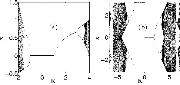
Figure 1: (a) The bifurcation diagram for the regular Logistic Map $x=Kx(1-x)$. (b) The bifurcation diagram for 1D Standard Map Eq. (17).

The bifurcation diagrams for the regular Logistic Map and the one-dimensional Standard Map are presented in Fig. 1.

The 1D Standard Map has the attracting fixed points $2\pi n$ for $0<K<2$ and $\pi+2\pi n$ when $-2<K<0$ (see Fig. 1b). The antisymmetric $T=2$ points are stable for $2<|K|<\pi$, while $x_{n+1}=x_{n}+\pi$ sinks ($T=2$) are stable when $\pi<|K|<\sqrt{\pi^{2}+2}\approx 3.445$. The stable $T=4$ sink appears at $K\approx 3.445$ and the transition to chaos through the period doubling cascade of bifurcations occurs at $K\approx 3.532$. More on the properties of the $\alpha=1$ Standard Map can be found in Edelman (2011a). .

Stability properties of the Logistic Map are well known May (1976a). For $K>0$, the $x=0$ fixed point is stable when $K<1$, the $(K-1)/K$ fixed point is stable when $1<K<3$,the $T=2$ sink is stable for $3\leq K<1-\sqrt{6}\approx 3.449$, the $T=4$ sink is stable for $3.449<K<3.544$, and at $K\approx 3.56995$ is the onset of chaos, at the end of the period-doubling cascade of bifurcations.

III.2 Two-Dimensional Maps

The regular ($\alpha=2$) Standard Map (Chirikov Standard Map)

$$p_{n+1}=p_{n}-K\sin x,\ \ \ \ ({\rm mod}\ 2\pi),$$

$$x_{n+1}=x_{n}+p_{n+1},\ \ \ \ ({\rm mod}\ 2\pi)$$ (18)

demonstrates a universal generic behavior of the area-preserving maps whose phase space is divided into elliptic islands of stability and areas of chaotic motion and is well investigated (see e.g. Chirikov (1979a)). In the S$\alpha$FM with $1<\alpha<2$ the elliptic islands evolve into periodic sinks Edelman and Tarasov (2009a); Edelman (2011a); Taieb ; Edelman (2011a). The properties of the phase space and the appearance of the CBTT in the S$\alpha$FM are connected to the evolution (with the increase in parameter $K$) of the regular Standard Map’s islands originating from the stable for $K<4$ fixed point (0,0). At $K=4$ it becomes unstable (elliptic-hyperbolic point transition) and two elliptic islands around the stable for $4<K<2\pi$ period 2 antisymmetric ($p_{n+1}=-p_{n}$, $x_{n+1}=-x_{n}$) point appear. At $K=2\pi$ this point turns into the $T=2$ point with $p_{n+1}=-p_{n}$, $x_{n+1}=x_{n}-\pi$ which is stable for $2\pi<K<6.59$. The $T=4$ stable elliptic points appear at $K\approx 6.59$ and the period doubling cascade of bifurcations leads to the disappearance of the islands of stability in the chaotic sea at $K\approx 6.6344$ Chirikov (1979a).

The $\alpha=2$ Logistic Map

$$p_{n+1}=p_{n}+Kx_{n}(1-x_{n})-x_{n},$$

$$x_{n+1}=x_{n}+p_{n+1}$$ (19)

is a quadratic area preserving map. The quadratic area preserving maps with a stable fixed point at the origin were studied by Hénon Henon (1969a) and a recent review on quadratic maps can be found in ZeraS2010 . The map Eq. (19) has two fixed points: $(0,0)$ stable for $K\in(-3,1)$ and $((K-1)/K,0)$ stable for $K\in(1,5)$. The $T=2$ elliptic point

$$x=\frac{K+3\pm\sqrt{(K+3)(K-5)}}{2K},$$

$$p=\pm\frac{\sqrt{(K+3)(K-5)}}{K}$$ (20)

is stable for $-2\sqrt{5}+1<K<-3$ and $5<K<2\sqrt{5}+1$. The period doubling cascade of bifurcations (for $K>0$) with further bifurcations, $T=2$ $\rightarrow$ $T=4$ at $K\approx 5.472$, $T=4$ $\rightarrow$ $T=8$ at $K\approx 5.527$, $T=8$ $\rightarrow$ $T=16$ at $K\approx 5.5319$, $T=16$ $\rightarrow$ $T=32$ at $K\approx 5.53253$, etc., and the corresponding decrease in the area of the islands of stability leads to chaos (see Fig. 2).

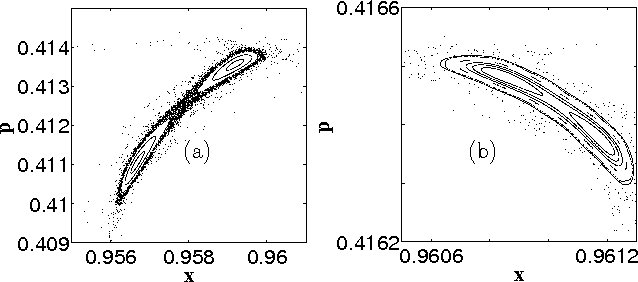
Figure 2: Bifurcations in the 2D Logistic Map: (a) $T=4$ $\rightarrow$ $T=8$ bifurcation at $K\approx 5.527$. (b) $T=8$ $\rightarrow$ $T=16$ bifurcation at $K\approx 5.5319$.

IV The Fractional ($\alpha<2$) S$\alpha$FM and L$\alpha$FM

IV.1 The CBTT in the S$\alpha$FM and the L$\alpha$FM with $\alpha<1$

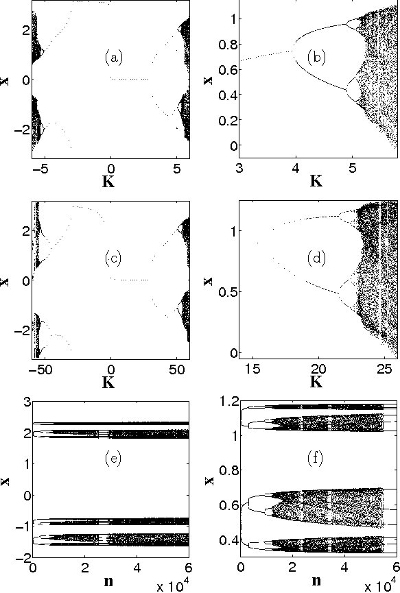
Figure 3: Bifurcations and the CBTT in the S$\alpha$CFM and the L$\alpha$CFM with $0<\alpha<1$. (a)-(d) bifurcation diagrams obtained after performing $10^{4}$ iterations on a single trajectory with $x_{0}=0.1$ for various values of $K$. (a) The S$\alpha$CFM with $\alpha=0.5$. (b) The L$\alpha$CFM with $\alpha=0.5$. (c) The S$\alpha$CFM with $\alpha=0.05$. (d) The L$\alpha$CFM with $\alpha=0.1$. (e) A CBTT in the S$\alpha$CFM with $\alpha=0.01$ and $K=276$. (f) A CBTT in the L$\alpha$CFM with $\alpha=0.1$ and $K=22.7$.

With the corresponding $G_{K}(x)$ the U$\alpha$CFM for $0<\alpha<1$

$$x_{n+1}=x_{0}-\frac{1}{\Gamma(\alpha)}\sum^{n}_{k=0}G(x_{k})(n-k+1)^{\alpha-1}$$ (21)

produces the S$\alpha$CFM

$$x_{n}=x_{0}-\frac{K}{\Gamma(\alpha)}\sum^{n-1}_{k=0}\frac{\sin{x_{k}}}{(n-k)^{1-\alpha}},\ \ ({\rm mod}\ 2\pi)$$ (22)

and the L$\alpha$CFM

$$x_{n}=x_{0}+\frac{1}{\Gamma(\alpha)}\sum^{n-1}_{k=0}\frac{Kx_{k}(1-x_{k})-x_{k}}{(n-k)^{1-\alpha}},$$ (23)

which are one dimensional maps with the power law decreasing memory Edelman (2011a). The bifurcation diagrams for these maps are similar to the corresponding diagrams for the $\alpha=1$ case but are stretched along the parameter $K$-axis and the stretchiness increases with the decrease in $\alpha$ Figs. 3(a)-(d). In the area of the parameter values for which on the bifurcation diagram stable periodic $T>2$ points exist individual trajectories are the CBTT Figs. 3(e),(f).

IV.2 The CBTT in the S$\alpha$FM with $1<\alpha<2$

The S$\alpha$RLFM and the S$\alpha$CFM with $1<\alpha<2$ were investigated in Edelman and Tarasov (2009a); Edelman (2011a); Taieb . In this subsection we’ll recall some of the results of this investigation. The fixed point $(0,0)$, which is a sink in this case, is stable for (see Fig. 4a)

$$0<K<K_{c1}(\alpha)=\frac{2\Gamma(\alpha)}{V_{\alpha l}},$$ (24)

where

$$V_{\alpha l}=\sum_{k=1}^{\infty}(-1)^{k+1}V_{\alpha}^{1}(k)\ \ .$$ (25)

In accordance with Sec. III $K_{c1}(1)=2$ and $K_{c1}(2)=4$.

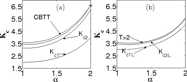
Figure 4: Bifurcations in the S$\alpha$FM and the L$\alpha$FM with $1<\alpha<2$. (a) The S$\alpha$FM $K-\alpha$ graph. The fixed point $(0,0)$ is stable for $K<K_{c1}$; the antisymmetric $T=2$ sink is stable for $K_{c1}<K<K_{c2}$; two $T=2$ sinks $x_{n+1}=x_{n}-\pi$, $p_{n+1}=-p_{n}$ are stable in a band above $K_{c2}$; the CBTT exist in the band of the map’s parameters ending at the cusp in the top right corner; the upper curve is a border with chaos. The star marks the point ($K\approx 6.63$) at which the Standard Map’s ($\alpha=2$) $T=2$ points become unstable and the $T=4$ elliptic points are born. (b) The L$\alpha$FM $K-\alpha$ graph. One fixed point is stable for $K<K_{c1L}$; the $T=2$ sink is stable for $K_{c1L}<K<K_{c2L}$; the sinks with $T\geq 4$ and the inverse CBTT exist in the upper band; the upper curve is a border with chaos.

The antisymmetric period 2 sink

$$p_{n+1}=-p_{n},\ \ x_{n+1}=-x_{n}$$ (26)

is stable for $K_{c1}(\alpha)<K<K_{c2}(\alpha)$ where $K_{c2}(\alpha)=0.5\pi K_{c1}(\alpha)$ with $K_{c2}(1)=\pi$ and $K_{c2}(2)=2\pi$.

$$p_{n+1}=-p_{n},\ \ x_{n+1}=x_{n}+\pi$$ (27)

two T=2 sinks are stable in the band above $K=K_{c2}(\alpha)$ curve (Fig. 4a). For $\alpha=1$ it corresponds to $\pi<|K|<\sqrt{\pi^{2}+2}\approx 3.445$ and for the regular Standard Map the corresponding elliptic points are stable when $2\pi<K<6.59$.

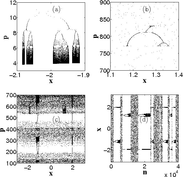
Figure 5: A single CBTT in the S$\alpha$RLFM. (a) One of the two branches of the CBTT for $\alpha=1.1,K=3.5$. (b) A zoom of a small feature in an intermittent trajectory for $\alpha=1.95,K=6.2$. (c) An intermittent trajectory in phase space for $\alpha=1.65,K=4.5$. (d) $x$ of $n$ for the case (c).

For $\alpha=1$ the $T=4$ sink appears at $K\approx 3.445$ and the transition to chaos occurs at $K\approx 3.532$ (Sec. III.1) while for $\alpha=2$ the $T=4$ elliptic points appear at $K\approx 6.59$ and the sequence of the period doubling bifurcations leads to the disappearance of the islands of stability in chaotic sea at $K\approx 6.6344$ (Sec. III.2). For $1<\alpha<2$ the CBTT exist in the band between two curves connecting the above-mentioned points (Fig. 4a). Both curves are calculated numerically and confirmed by the large number of computer simulations Edelman (2011a); Taieb . Within the CBTT band trajectories evolve from being very stable features which exist for the longest time we were running our codes, 500000 iterations, when $\alpha$ is close to 1 (Fig. 5a) to being barely distinguishable and short-lived features when $\alpha$ is close to 2 (Fig. 5b). For the intermediate values of $\alpha$ CBTT behave similar to the sticky trajectories in Hamiltonian dynamics: occasionally trajectories enter CBTT and then leave them entering the chaotic sea (Figs. 5c, d).

Let’s list below some additional interesting properties of the S$\alpha$FM with $1<\alpha<2$ Edelman (2011a); Taieb . The types of solutions include periodic sinks, attracting slow diverging trajectories, attracting accelerator mode trajectories, chaotic attractors, and the CBTT. All attractors below the CBTT band are periodic sinks and slow diverging trajectories and all trajectories converge to one of those attractors. Each attractor has its own basin of attraction and the chaotic areas exist in the sense that two trajectories with infinitely close initial conditions from those areas may converge to different attractors. Periodic sinks exist in the limiting sense and the limiting values themselves in most of the cases do not belong to their basins of attraction. The rate of convergence of trajectories to the sinks depends on the initial conditions. The trajectories which start from the basins of attraction converge fast as $\delta x\sim n^{-1-\alpha}$, $\delta p\sim n^{-\alpha}$, while those starting from the chaotic areas converge slow as $\delta x\sim n^{-\alpha}$ (or even as $\delta x\sim n^{1-\alpha}$), $\delta p\sim n^{1-\alpha}$. Trajectories may intersect and chaotic attractors overlap. More on the properties of the S$\alpha$RLFM and the S$\alpha$CFM for $1\leq\alpha\leq 2$ can be found in Edelman (2011a); Taieb ; Edelman (2011a).

IV.3 CBTT in L$\alpha$FM with $1<\alpha<2$

In this part we’ll investigate the L$\alpha$RLFM

$$p_{n+1}=p_{n}+Kx_{n}(1-x_{n})-x_{n},$$ (28)

$$x_{n+1}=\frac{1}{\Gamma(\alpha)}\sum_{i=0}^{n}p_{i+1}V^{1}_{\alpha}(n-i+1).$$ (29)

As in the case of the S$\alpha$FM, the partition of the phase space into the areas of stability of the periodic sinks originating from the period one sink $(0,0)$ is almost the same (numerical result) for the L$\alpha$RLFM and the L$\alpha$CFM. For $0<K<1$ all converging trajectories converge to $(0,0)$ point as $x\sim n^{-\alpha-1}$, $p\sim n^{-\alpha}$. For $1<K<K_{c1L}$ the only stable sink is the period one $((K-1)/K,0)$ sink and the rate of convergence is $\delta x\sim n^{-\alpha}$, $p\sim n^{-\alpha+1}$. For $K_{c1L}<K<K_{c2L}$ all converging trajectories (this is a result from the large number of numerical simulations) converge to the $T=2$ sink antisymmetric in $p$ Fig. 6a.

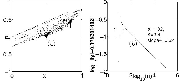
Figure 6: The L$\alpha$RLFM with $\alpha=1.32$, $K=3.4$. (a) Phase space: 300 trajectories with $x_{0}=0$, $p_{0}=10^{-6}+0.00024i$, $0\leq i<300$. All converging trajectories converge to the $T=2$ antisymmetric in $p$ sink. (b) $\log p-\log n$ graph showing the rate of convergence $\delta p\approx n^{-\alpha+1}$ on a single trajectory.

To find the L$\alpha$RLFM’s critical curve $K_{c1L}$ on which, as a result of a bifurcation, the $T=1$ sink disappears and the $T=2$ sink is born, let’s consider the $T=2$ sinks. The results of large number of simulations (see e.g. Fig. 6b) suggest the following asymptotic behavior:

$$p_{n}=p_{l}(-1)^{n}+\frac{A}{n^{\alpha-1}}\ \ .$$ (30)

Then, from Eq. (29)

$$x_{lo}=\lim_{n\rightarrow\infty}x_{2n+1}=\frac{p_{l}}{\Gamma(\alpha)}\lim_{n\rightarrow\infty}\sum^{2n+1}_{k=1}(-1)^{k}V_{\alpha}^{1}(k)$$

$$+\frac{A}{\Gamma(\alpha)}\lim_{n\rightarrow\infty}\sum^{2n-1}_{k=1}\frac{\alpha-1}{k^{\alpha-1}(2n-k)^{2-\alpha}}=-\frac{p_{l}}{\Gamma(\alpha)}V_{\alpha l}$$ (31)

$$+\frac{(\alpha-1)A}{\Gamma(\alpha)}\int^{1}_{0}\frac{x^{1-\alpha}dx}{(1-x)^{2-\alpha}}=-\frac{p_{l}}{\Gamma(\alpha)}V_{\alpha l}+A\Gamma(2-\alpha).$$

In a similar way

$$x_{le}=\lim_{n\rightarrow\infty}x_{2n}=\frac{p_{l}}{\Gamma(\alpha)}V_{\alpha l}+A\Gamma(2-\alpha).$$ (32)

In the limit $n\rightarrow\infty$ Eq. (28) gives

$$-2p_{l}=Kx_{le}(1-x_{le})-x_{le},$$ (33)

$$2p_{l}=Kx_{lo}(1-x_{lo})-x_{lo}.$$ (34)

The system of Eqs. (31)-(34) has four equations and four unknown variables $p_{l}$, $A$, $x_{lo}$, and $x_{le}$. This equation has two obvious solutions $x_{lo}=x_{le}=p_{l}=A=0$ and $x_{lo}=x_{le}=x_{l}=(K-1)/K$, $p_{l}=0$, $A=x_{l}/\Gamma(2-\alpha)$, corresponding to two fixed points. If $x_{lo}\neq x_{le}$, then

$$A=\frac{K-1+\frac{2\Gamma(\alpha)}{V_{\alpha l}}}{2K\Gamma(2-\alpha)}$$ (35)

and $x_{le}$ is a solution of the quadratic equation

$$x_{le}^{2}-\Bigl{(}\frac{2\Gamma(\alpha)}{KV_{\alpha l}}+\frac{K-1}{K}\Bigr{)}x_{le}+\Bigl{(}\frac{\Gamma(\alpha)}{2KV_{\alpha l}}+\frac{K-1}{4K}\Bigr{)}^{2}$$

$$-\frac{(K-1)\Gamma(\alpha)}{K^{2}V_{\alpha l}}-\frac{(K-1)^{2}}{2K^{2}}=0,$$ (36)

which for positive $K$ has solutions only when

$$K\geq K_{c1l}=1+\frac{2\Gamma(\alpha)}{V_{\alpha l}}.$$ (37)

Direct numeric simulations of the map Eqs. (28) and (29) confirm this $K_{c1l}$ value as well as the limiting values for $p_{l}$, $x_{lo}$, and $x_{le}$. For a way to calculate numerically slow converging series Eq. (25) for $V_{\alpha l}$ see APPENDIX.

In the CBTT band of the L$\alpha$FM, the narrow band between the upper two curves on Fig. 4b, the cascade of bifurcation type trajectories exist only in the form of the inverse CBTT (see Fig. 7). The inverse CBTT which exist for the L$\alpha$CFM (Figs. 7 and 8a) are almost impossible to find in the L$\alpha$RLFM (Fig. 8b). The closer $\alpha$ is to two the more difficult it is to find the CBTT in the phase space or $x$-$n$ graph of the L$\alpha$CFM.

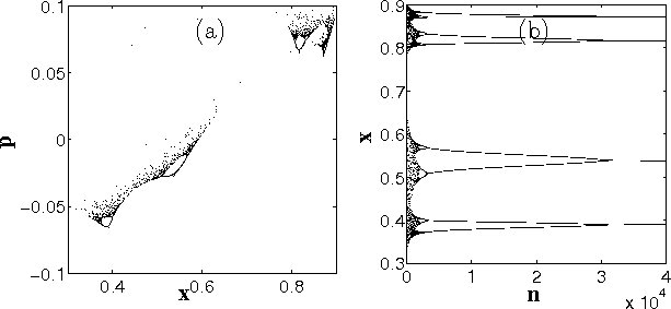
Figure 7: An inverse CBTT in the L$\alpha$CFM with $\alpha=1.2$, $K=3.45$. 40000 iterations on a trajectory with $x_{0}=0.01$ and $p_{0}=0.1$. (a) Phase space. (b) $x-n$ graph.

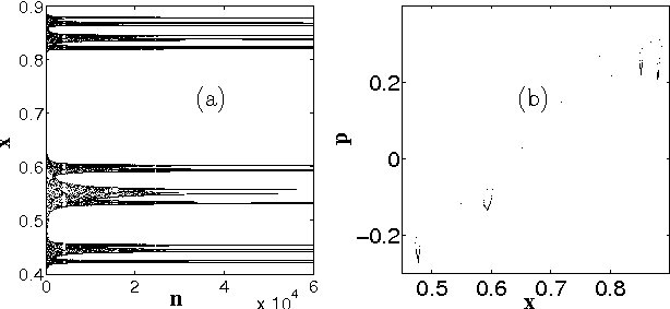
Figure 8: The L$\alpha$CFM vs. the L$\alpha$RLFM. (a) 60000 iterations on a single L$\alpha$CFM trajectory for $\alpha=1.6$ $K=3.9$ (b) the $T=4$ trajectory for the L$\alpha$RLFM with $\alpha=1.6$ $K=3.88$.

V Conclusion

The Universal $\alpha$-Family of Maps introduced in this paper is the extension of the fractional Universal Map, which allows consideration of the Logistic Map as its particular form. The results of the investigation of the Standard and Logistic Families of Maps suggest that the existence of the cascade of bifurcations type trajectories is a general property of the fractional dynamical systems. They appear for the parameter values corresponding to the transition through the period doubling cascade of bifurcations from regular to chaotic motion in the regular dynamics. Fig. 3 and Fig. 5 support our statement that with the increase in $\alpha$, which represents the increase in the systems’ dimension and memory (increase in the weights of the earlier states), systems demonstrate more complex and chaotic behavior. Biological systems are systems with memory and the Fractional Logistic Map can serve as a basic model in population biology with memory. We believe that experiments on human memory and/or adaptive biological systems, which in many respects are systems with power law memory, could demonstrate the CBTT-like behavior. New types of materials with memory, such as memristors, memcapacitors, and meminductors, could be used to model fractional systems to demonstrate the existence of the CBTT. The $\alpha>2$ Standard and Logistic Maps (including their integer volume preserving forms) are topics of ongoing research and their further investigation is necessary to demonstrate the consistency of the changes in the properties of the fractional systems with the change in $\alpha$.

Appendix

$V_{\alpha l}$ can be written as

$$V_{\alpha l}=\sum_{k=1}^{\infty}(-1)^{k+1}V_{\alpha}(k)=S_{1}+S_{2},$$ (38)

where

$$S_{1}=\sum_{k=1}^{2N}(-1)^{k+1}V_{\alpha}(k)$$ (39)

with the $N$ sufficiently large and

$$S_{2}=\sum_{k=N+1}^{\infty}\{V_{\alpha}(2k-1)-V_{\alpha}(2k)\}\ \ .$$ (40)

The value of $S_{1}$ can be directly calculated numerically with high precision. The second sum can be developed into a series as follows

$$S_{2}=\sum_{k=N+1}^{\infty}(2k)^{\alpha-3}(\alpha-1)(2-\alpha)\Bigl{(}1+\frac{3-\alpha}{2}\frac{1}{k}$$

$$+\frac{7(3-\alpha)(4-\alpha)}{48}\frac{1}{k^{2}}+\frac{(3-\alpha)(4-\alpha)(5-\alpha)}{32}\frac{1}{k^{3}}+O(\frac{1}{k^{4}})\Bigr{)}$$

$$=(2)^{\alpha-3}(\alpha-1)(2-\alpha)\Bigl{(}\zeta(3-\alpha)+\frac{3-\alpha}{2}\zeta(4-\alpha)+$$ (41)

$$\frac{7(3-\alpha)(4-\alpha)}{48}\zeta(5-\alpha)+\frac{(3-\alpha)(4-\alpha)(5-\alpha)}{32}\zeta(6-\alpha)\Bigr{)}$$

$$-\sum_{k=1}^{N}(2k)^{\alpha-3}(\alpha-1)(2-\alpha)\Bigl{(}1+\frac{3-\alpha}{2}\frac{1}{k}+\frac{7(3-\alpha)(4-\alpha)}{48}\frac{1}{k^{2}}$$

$$+\frac{(3-\alpha)(4-\alpha)(5-\alpha)}{32}\frac{1}{k^{3}}\Bigr{)}+O(\frac{1}{N^{6-\alpha}}).$$

This is what finally was coded using a fast method for calculating values of the $\zeta$-function.

References

- (1) S. G. Samko, A. A. Kilbas, O. I. Marichev, Fractional Integrals and Derivatives Theory and Applications (Gordon and Breach, New York, 1993).
- (2) I. Podlubny, Fractional Differential Equations, (Academic Press, San Diego, 1999).
- (3) A. A. Kilbas, H. M. Srivastava, J. J. Trujillo, Theory and Application of Fractional Differential Equations (Elsevier, Amsterdam, 2006).
- (4) G. M. Zaslavsky, Hamiltonian Chaos and Fractional Dynamics (Oxford University Press, Oxford, 2005).
- (5) R. Hilfer (Ed.), Applications of Fractional Calculus in Physics (World Scientific, Singapore, 2000).
- (6) J. Sabatier, 0. P. Agraval, J. A. Tenreiro Machado (Eds.), Advances in Fractional Calculus. Theoretical Developments and Applications in Physics and Engineering (Springer, Dordrecht, 2007).
- (7) V. E. Tarasov, Fractional Dynamics: Application of Fractional Calculus to Dynamics of Particles, Fields, and Media (Springer, HEP, Beijing, 2011).
- (8) V. V. Uchaikin, Fractional Derivatives for Physicists and Engineers (Springer, HEP, Heidelberg, 2013).
- (9) I. Petras, Fractional-Order Nonlinear Systems (Springer, HEP, Beijing, 2011).
- (10) I. Pan, S. Das, Intelligent Fractional Order Systems and Control: An Introduction (Studies in Computational Intelligence) (Springer, Heidelberg, 2013).
- (11) F. Mainardi, Fractional Calculus and Waves in Linear Viscoelasticity: An Introduction to Mathematical Models (Imperial College Press, London, 2010).
- Tarasov (2008a) V. E. Tarasov, Journal of Physics: Condensed Matter 20, 145212 (2008).
- Tarasov (2008a) V. E. Tarasov, Journal of Physics: Condensed Matter 20, 175223 (2008).
- Tarasov (2009a) V. E. Tarasov, Theor. and Math. Phys. 158, 355 (2009).
- Lundstrom, Fairhall (2008a) B. N. Lundstrom, A. L. Fairhall, and M. Maraval, J. Neuroscience 30, 5071 (2010).
- Lundstrom, Higgs (2008a) B. N. Lundstrom, M. H. Higgs, W. J. Spain, and A. L. Fairhall, Nature Neuroscience 11, 1335 (2008).
- Wixted and Ebbesen (1997a) J. T. Wixted and E. Ebbesen, Mem. Cognit. 25, 731 (1997).
- Toib, Lyakhov (1998a) A. Toib, V. Lyakhov, and S. Marom, J. Neuroscience 18, 1893 (1998).
- Fairhall, Lewen (2001a) A. L. Fairhall, G. D. Lewen, W. Bialek, and R. R. de Ruyter van Steveninck, Nature 412, 1335 (2001).
- Leopold, Murayama (2003a) D. A. Leopold, Y. Murayama, and N. Logothetis, Cereb. Cortex 13, 422 (2003).
- Ulanovsky, Las (2004a) N. Ulanovsky, L. Las, D. Farkas, and I. Nelken, J. Neuroscience 24, 10440 (2004).
- Zilany, Bruce (2009a) M. S. A. Zilany, I. C. Bruce, P. C. Nelson, and L. H. Carney, J. Acoust. Soc. Am. 126, 2390 (2009).
- Min, Luo (2005a) W. Min, G. Luo, B. J. Cherayil, S. C. Kou, and X. S. Xie, P.R.L. 94, 198302 (2005).
- Wixted (1990a) J. T. Wixted, J. Exp. Psychol.: Learn., Mem. Cognit. 16, 927 (1990).
- Wixted and Ebbesen (1990a) J. T. Wixted and E. Ebbesen, Psychol. Sci. 2, 409 (1990).
- Rubin and Wenzel (1996a) D. C. Rubin and A. E. Wenzel, Psychol. Rev. 103, 734 (1996).
- (27) M. J. Kahana, Foundations of human memory (Oxford University Press, New York, 2012).
- (28) J. R. Anderson, Learning and memory: An integrated approach (Wiley, New York, 1995).
- Kilbas, Bonilla, and Trujillo (2000a) A. A. Kilbas, B. Bonilla, and J. J. Trujillo, Doklady Mathematics 62, 222 (2000a); Demonstratio Mathematica 33, 583 (2000b).
- Tarasov (2009a) V. E. Tarasov, J. Math. Phys. 50, 122703 (2009a); J. Phys. A 42, 465102 (2009b).
- Wineman (2007a) A. Wineman, Comput. Math. Appl. 53, 168 (2007a).
- Wineman (2009a) A. Wineman, Mathematics and Mechanics of Solids 14, 300 (2009a).
- (33) F. Hoppensteadt, Mathematical Theories of Populations: Demographics, Genetics, and Epidemics (SIAM, Philadelphia, 1975).
- (34) F. Brauer, C. Castillo-Chavez, Mathematical Models in Population Biology and Epidemiology (Springer, New York, 2001).
- (35) D. K. Arrowsmith and C. M. Place, An introduction to dynamical system (Cambridge University Press, Cambridge, 1990 ); M. Feigenbaum, J. Stat. Phys. 19, 25 (1978a); O. E. Landford, Bul. Am. Math. Soc. 6, 427 (1982a); E. B. Vul, Y. G. Sinai, and K. M. Khanin, Russ. Math. Surv. 39, 1 (1984); P. Cvitanovic, Universality in chaos (Adam Hilger, Bristol, 1989).
- (36) R. Caponetto, G. Dongola, L. Fortuna, and I. Petras, Fractional Order Systems: Modeling and Control Applications (World Scientific Series on Nonlinear Science Series a) (World Scientific, Singapore, 2010).
- Chua (1971a) L. O. Chua, IEEE Trans. Circuit Theory 18, 507 (1971a).
- Di Ventra (2009a) M. Di Ventra, Y. V. Pershin and L. O Chua, Proc. IEEE 97, 1717 (2009).
- Tenreiro Machado (2013a) J. Trenreiro Machado, Commun. Nonlin. Sci. Numer. Simul. 18, 264 (2013a).
- Cafagna and Grassi (2012a) D. Cafagna and G. Grassi, Nonlin. Dyn. 70, 1185 (2012).
- Tarasov and Zaslavsky (2008a) V. E. Tarasov and G. M. Zaslavsky, J. Phys. A 41, 435101 (2008).
- Edelman and Tarasov (2009a) M. Edelman and V. E Tarasov, Phys. Let. A 374, 279 (2009).
- Tarasov and Edelman (2010a) V. E. Tarasov and M. Edelman, Chaos 20, 023127 (2010).
- Edelman (2011a) M. Edelman, Commun. Nonlin. Sci. Numer. Simul. 16, 4573 (2011a).
- (45) M. Edelman and L. A. Taieb, in: Advances in Harmonic Analysis and Operator Theory; Series: Operator Theory: Advances and Applications, edited by A. Almeida, L. Castro, and F.-O. Speck, vol. 229, pp. 139-155 (Springer, Basel, 2013).
- Edelman (2011a) M. Edelman, Discontinuity, Nonlinearity, and Complexity 1, 305 (2013a).
- Fulinski,Kleczkowski (1987a) A. Fulinski, A. S. Kleczkowski, A. Fulinski and A. S. Kleczkowski, Physica Scripta 35, 119 (1987a); E. Fick, M. Fick, and G. Hausmann, Phys. Rev. A. 44, 2469 (1991a); K. Hartwich and E. Fick, Phys. Lett. A 177, 305 (1993); M. Giona, Nonlinearity 4, 911 (1991); J. A. C. Gallas, Physica A 198, 339 (1993); A. A. Stanislavsky, Chaos 16, 043105 (2006).
- Meiss (2012a) H. R. Dullin and J. D. Meiss, SIAM J. Appl. Dyn. Sys. 11, 319 (2012a); J. D. Meiss, Commun. Nonlin. Sci. Numer. Simul. 17, 2108 (2016a).
- Moser (1994a) J. Moser, Math. Z. 216, 417 (1994); H. E. Lomeli and J. D. Meiss, Nonlinearity 11, 557 (1998a).
- May (1976a) R. M. May, Nature 261, 459 (1976a).
- Chirikov (1979a) B. V. Chirikov, Phys. Rep. 52, 263 (1979a); A. J. Lichtenberg, M. A. Lieberman, Regular and Chaotic Dynamics (Springer, Berlin, 1992).
- Henon (1969a) M. H. Hénon, Q. Appl. Math XXVII, 291 (1969).
- (53) E. Zeraoulia and J. C. Sprott, 2-D Quadratic Maps and 3-D ODE Systems: A Rigorous Approach (World Scientific, Singapore, 2010).