Fractal Continuation

Abstract.

A fractal function is a function whose graph is the attractor of an iterated function system. This paper generalizes analytic continuation of an analytic function to continuation of a fractal function.

1. Introduction

Analytic continuation is a central concept of mathematics. Riemannian geometry emerged from the continuation of real analytic functions. This paper generalizes analytic continuation of an analytic function to continuation of a fractal function. By fractal function, we mean basically a function whose graph is the attractor of an iterated function system. We demonstrate how analytic continuation of a function, defined locally by means of a Taylor series expansion, generalises to continuation of a, not necessarily analytic, fractal function.

Fractal functions have a long history, see [15] and [9, Chapter 5]. They were introduced, in the form considered here, in [1]. They include many well-known types of non-differentiable functions, including Takagi curves, Kiesswetter curves, Koch curves, space-filling curves, and nowhere differentiable functions of Weierstrass. A fractal function is a continuous function that maps a compact interval $I\subset\mathbb{R}$ into a complete metric space, usually $\mathbb{R}$ or $\mathbb{R}^{2}$, and may interpolate specified data and have specified non-integer Minkowski dimension. Fractal functions are the basis of a constructive approximation theory for non-differentiable functions. They have been developed both in theory and applications by many authors, see for example [3, 8, 9, 11, 12, 13, 14] and references therein.

Let $N$ be an integer and $\mathcal{I=\{}1,2,...,N\}$. Let $M\geq 2$ be an integer and $\mathbb{X\subset R}^{M}$ complete with respect to a metric $d_{\mathbb{X}}$ that induces, on $\mathbb{X}$, the same topology as the Euclidean metric. Let $\mathcal{W}$ be an iterated function system (IFS) of the form

(1 ) $$\mathcal{W}=\{\mathbb{X};w_{n},n\in\mathcal{I\}}\text{, }$$

We say that $\mathcal{W}$ is an analytic IFS if $w_{n}$ is a homeomorphism from ${\mathbb{X}}$ onto ${\mathbb{X}}$ for all $n\in\mathcal{I}$, and $w_{n}$ and its inverse $w_{n}^{-1}$ are analytic. By $w_{n}$ analytic, we mean that

$$w_{n}(x)=(w_{n1}(x),w_{n2}(x),...,w_{nM}(x)),$$

where each real-valued function $w_{nm}(x)=w_{nm}(x_{1},x_{2},...,x_{M})$ is infinitely differentiable in $x_{i}$ with $x_{j}$ fixed for all $j\neq i$, with a convergent multivariable Taylor series expansion convergent in a neigbourhood of each point $(x_{1},x_{2},...,x_{M})\in\mathbb{X}$.

To introduce the main ideas, define a fractal function as a continuous function $f:I\rightarrow\mathbb{R}^{M-1}$, where $I\subset\mathbb{R}$ is a compact interval whose graph $G(f)$ is the attractor of a IFS for the form in eqaution (1). A slightly more restrictive definition will be given in Section 3. If $\mathcal{W}$ is an analytic IFS, then $f$ is called an analytic fractal function.

The adjective “fractal” is used to emphasize that $G(f)$ may have noninteger Hausdorff and Minkowski dimensions. But $f$ may be many times differentiable or $f$ may even be a real analytic function. Indeed, we prove that all real analytic functions are, locally, analytic fractal functions; see Theorem 4.2. An alternative name for a fractal function $f$ could be a “self-similar function” because $G(f)$ is a union of transformed “copies” of itself, specifically

(2 ) $$G(f)=\bigcup_{n=1}^{N}w_{n}(G(f)).$$

The goal of this paper is to introduce a new method of analytic continuation, a method that applies to fractal functions as well as analytic functions. We call this method fractal continuation. When fractal continuation is applied to a locally defined real analytic function, it yields the standard analytic continuation. When fractal continuation is applied to a fractal function $f$, a set of continuations is obtained. We prove that, in the generic situation with $M=N=2$, this set of continuations depends only on the function $f$ and is independent of the particular IFS $\mathcal{W}$ that was used to produce $f$. The proof relies on the detailed geometrical structure of analytic fractal functions and on the Weierstass preparation theorem.

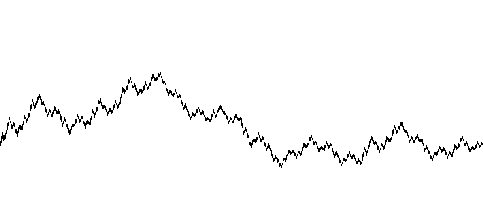
Figure 1. This paper concerns analytic continuation, not only of analytic functions, but also of non-differentiable functions such as the one whose graph is illustrated here.

The spirit of this paper is summarized in Figure 1. Basic terminology and background results related to iterated function systems appear in Section 2. In Section 3 we establish the existence of fractal functions whose graphs are the attractors of a general class of IFS, which we call an interpolation IFS. An analytic fractal function is a fractal function whose graph is the attractor of an analytic interpolation IFS. This includes the popular case of affine fractal interpolation functions [1]. An analytic function is a special case of an analytic fractal function, as proved in Section 4. Fractal continuation, the main topic of this paper, is introduced in Section 5. The fractal continuation of an analytic function is the usual analytic continuation. In general, however, a fractal function defined on a compact domain, has infinitely many continuations, this set of continuations having a fascinating geometric structure as demonstrated by the examples that are also contained in Section 5. The graph of a given fractal function can be the attractor of many distinct analytic IFSs. We conjecture that the set of fractal continuations of a function whose graph is the attractor of an analytic interpolation IFS is independent of the particular IFS. Some cases of this uniqueness result are proved in Section 6.

2. Iterated Function Systems

An iterated function system (IFS)

$$\mathcal{W=\{}\mathbb{X};w_{n},n\in\mathcal{I}\}$$

consists of a complete metric space $\mathbb{X\subset R}^{M}$ with metric $d_{\mathbb{X}},$ and $N$ continuous functions $w_{n}:\mathbb{X}\rightarrow\mathbb{X}$. The IFS $\mathcal{W}$ is called contractive if each function $w$ in $\mathcal{W}$ is a contraction, i.e., if there is a constant $s\in[0,1)$ such that

$$d(w(x),w(y))\leq s\,d(x,y)$$

for all $x,y\in\mathbb{X}$. The IFS $\mathcal{W}$ is called an invertible IFS if each function in $\mathcal{W}$ is a homeomorphism of ${\mathbb{X}}$ onto ${\mathbb{X}}$. The definition of analytic IFS is as given in the introduction. The IFS $\mathcal{W}$ is called an affine IFS if $\mathbb{X=R}^{M}$ and $w_{n}:\mathbb{R}^{M}\rightarrow\mathbb{R}^{M}$ is an invertible affine map for all $n\in\mathcal{I}$. Clearly an affine IFS is analytic, and an analytic IFS is invertible.

The set of nonempty compact subsets of $\mathbb{X}$ is denoted $\mathbb{H}=\mathbb{H}(\mathbb{X})$. It is well-known that $\mathbb{H}$ is complete with respect to the Hausdorff metric $h$, defined for all $S,T\in\mathbb{H}$, by

$$h(S,T)=\max\,\left\{\underset{s\in S}{\max}\,\underset{t\in T}{\min}\,d_{\mathbb{X}}(s,t),\underset{t\in T}{\max}\,\underset{s\in S}{\min}\,d_{\mathbb{X}}(s,t)\right\}\text{.}$$

Define $\mathcal{W}:\mathbb{H\rightarrow H}$ by

(3 ) $$\mathcal{W}\mathcal{(}K)=\bigcup\limits_{n\in\mathcal{I}}w_{n}(K)$$

for all $K\in\mathbb{H}$. Let $\mathcal{W}^{0}:\mathbb{H\rightarrow H}$ be the identity map, and let $\mathcal{W}^{k}:\mathbb{H}\mathbb{\rightarrow H}$ be the $k$-fold composition of $\mathcal{W}$ with itself, for all integers $k>0.$

Definition 2.1.

A set $A\in\mathbb{H}$ is said to be an attractor of $\mathcal{W}$ if ${\mathcal{W}}(A)=A$, and

(4 ) $$\lim_{k\rightarrow\infty}\mathcal{W}^{k}(K)=A$$

for all $K\in\mathbb{H}$, where the convergence is with respect to the Hausdorff metric.

A basic result in the subject is the following [7].

Theorem 2.2.

If IFS $\mathcal{W}$ is contractive, then $\mathcal{W}$ has a unique attractor.

The remainder of this section provides the definition of a certain type of IFS whose attractor is the graph of a function. We call this type of IFS an interpolation IFS. We mainly follow the notation and ideas from [1, 2, 3].

Let $M\geq 2$ and $N$ an integer and $\mathcal{I=\{}1,2,...,N\}$. For a sequence $x_{0}<x_{1}<\cdots<x_{N}$ of real numbers, let $L_{n}:\mathbb{R\rightarrow R}$ be the affine function and $F_{n}:{\mathbb{R}}\times{\mathbb{R}}^{M-1}\rightarrow\ R^{M-1},\;n=1,2,\dots,N$ be a continuous function satisfying the following properties:

1. $L_{n}(x_{0})=x_{n-1}$ and $L_{n}(x_{N})=x_{n}$.

2. There are points $y_{0}$ and $y_{N}$ in $\mathbb{R}^{M-1}$ such that $F_{1}(x_{0},y_{0})=y_{0}$ and $F_{N}(x_{N},y_{N})=y_{N}$.

3. $F_{n+1}(x_{0},y_{0})=F_{n}(x_{N},y_{N})$ for $n=1,2,\dots,N-1$.

Let $\mathcal{W}$ be the IFS

(5 ) $$\mathcal{W}=\{{\mathbb{R}}^{M}\,;\,w_{n},\,n\in\mathcal{I\}}\text{, }$$

where

(6 ) $$w_{n}(x,y)=(L_{n}(x),F_{n}(x,y)).$$

Keeping condition (c) in mind, if we define, for each $n\in\mathcal{I}$,

$$y_{n}:=F_{n+1}(x_{0},y_{0})=F_{n}(x_{N},y_{N}),$$

then note that

(7 ) $$w_{n}(x_{0},y_{0})=(x_{n-1},y_{n-1})\qquad\text{and}\qquad w_{n}(x_{N},y_{N})=(x_{n},y_{n}).$$

Definition 2.3.

An interpolation IFS is an IFS of the form given by (5) and (6) above that satisfies (1) $w_{n}$ is a homeomorphism onto its image for all $n\in\mathcal{I}$, and (2) there is an $s\in[0,1)$ and an $\mathcal{M}\in[0,\infty)$ such that

(8 ) $$|F_{n}(x,y)-F_{n}(x^{\prime},y^{\prime})|\leq\mathcal{M}|x-x^{\prime}|+s|y-y^{\prime}|$$

for all $x,x^{\prime}\in\mathbb{R},y,y^{\prime}\in{\mathbb{R}}^{M-1}$ and for all $n\in\mathcal{I}$. The term “interpolation” is justified by statement (2) in Theorem 3.2 in the next section.

3. Fractal Functions and Interpolation

Properties of an interpolation IFS are discussed in this section. Theorem 3.2 is the main result.

Lemma 3.1.

If $\mathcal{W}$ is an interpolation IFS, then $\mathcal{W}$ is contractive with respect to a metric inducing the same topology as the Euclidean metric on ${\mathbb{R}}^{M}$.

Proof.

Let $L_{n}=a_{n}x+b_{n}$ and let $d$ be the metric on $\mathbb{R}^{M}$ defined by

$$d((x,y),(x^{\prime},y^{\prime}))=e|x-x^{\prime}|+|y-y^{\prime}|$$

where $e\in(\mathcal{M}/(1-a),\infty)$ and $a=\max\{a_{n}:n\in\mathcal{I\}}$. The metric $d$ is a version of the ”taxi-cab” metric and is well-known to induce the usual topology on $\mathbb{R}^{M}$. Moreover, $w_{n}$ is a contraction with respect to the metric $d$: for $(x,y),(x^{\prime},y^{\prime})\in{\mathbb{R}}\times\mathbb{R}^{M-1}$,

$$d(w_{n}(x,y),w_{n}(x^{\prime},y^{\prime})) =e|L(x)-L(x^{\prime})|+|F_{n}(x,y)-F_{n}(x^{\prime},y^{\prime})|$$

$$\leq ea|x-x^{\prime}|+\mathcal{M}|x-x^{\prime}|+s|y-y^{\prime}|\text{ }$$

$$=\left(ea+\mathcal{M}\right)|x-x^{\prime}|+s|y-y^{\prime}|$$

$$=ce|x-x^{\prime}|+s|y-y^{\prime}|$$

$$\leq\max\{c,s\}\,d((x,y),(x^{\prime},y^{\prime}))$$

where $c=a+\mathcal{M}/e$ is monotone strictly decreasing function of $e$ for $e>0$, so $c$ is strictly less than $a+\mathcal{M}/(\mathcal{M}/(1-a))=1$ for $e\in(\mathcal{M}/(1-a),\infty).$    

Theorem 3.2 generalizes results such as [9, p.186, Theorem 5.4]. Let $I=[x_{0},x_{N}]$, $C(I)=\{f:I\rightarrow\mathbb{R}^{M-1}:f$ is continuous$\}$ and $C_{0}(I):=\{g\in C(I):g(x_{0})=y_{0},g(x_{N})=y_{N}\}.$

Theorem 3.2.

If $\mathcal{W}$ is an interpolation IFS, then

1. The IFS $\mathcal{W}$ has a unique attractor $G:=G(f)$ that is the graph of a continuous function $f\,:\,I\rightarrow{\mathbb{R}}^{M-1}$.

2. The function $f$ interpolates the data points $(x_{0},y_{0}),(x_{1},y_{1}),\dots,(x_{N},y_{N})$, i.e., $f(x_{n})=y_{n}$ for all $n$.

3. If $W\,:\,C_{0}(I)\rightarrow C_{0}(I)$ is defined by $(Wg)(x)=F_{n}(L_{n}^{-1}(x),g(L_{n}^{-1}(x)))$ for $x\in[x_{n-1},x_{n}]$, for $n\in\mathcal{I}$, and for all $g\in C_{0}(I)$, then $W$ has a unique fixed point $f$ and

   $$f=\lim_{n\rightarrow\infty}W^{k}(f_{0})$$

   for any $f_{0}\in C_{0}(I)$.

Proof.

It is readily checked that the mapping $\mathcal{W}$ of equation (3) takes $C_{0}(I)$ into $C_{0}(I)$ and also that the mapping $W$ of statement (3) in Theorem 3.2 takes $C_{0}(I)$ into $C_{0}(I).$ Moreover, if $G(f_{0})$ is the graph of the function $f_{0}\in C_{0}(I)$, then ${\mathcal{W}}(G(f_{0}))=W(f_{0})$. This implies, by property (4) of the attractor, that the function $f$ in statement (1), assuming that it exists, is the same as the function $f$ of statement (3), assuming that it exists. Statement (3) is proved first.

(3): That the map $W$ is a contraction on $C_{0}(I)$ with respect to the sup norm can be seen as follows. For all $g\in C_{0}(I)$,

$$|(Wg_{1})(x)-(Wg_{2})(x)| \leq\max_{n\in\mathcal{I}}|F_{n}(L_{n}^{-1}(x),g_{1}(L_{n}^{-1}(x)))-F_{n}(L_{n}^{-1}(x),g_{2}(L_{n}^{-1}(x)))|$$

$$\leq\max_{n\in\mathcal{I}}s\,|g_{1}(L_{n}^{-1}(x))-g_{2}(L_{n}^{-1}(x))|$$

$$\leq s\,\left|g_{1}(x)-g_{2}(x)\right|,$$

where $0\leq s<1$ is the constant in condition (8). Statement (3) now follows from the Banach contraction mapping theorem.

(1): According to Lemma 3.1, the IFS $\mathcal{W}$ is contractive. By Theorem 2.2, $\mathcal{W}$ has a unique attractor $G$. Let $G_{0}$ denote the graph of some function $f_{0}$ in $C_{0}(I)$. Using statement (3) there is a function $f\in C_{0}(I)$ such that $f=\lim_{k\rightarrow\infty}W^{k}(f_{0})$. By what was stated in the first paragraph of this proof and by the property (4) in the definition of attractor, we have $G=\lim_{k\rightarrow\infty}{\mathcal{W}}^{k}(G_{0})=G(\lim_{k\rightarrow\infty}W^{k}(f_{0}))=g(f)$.

(2): The attractor $G$ must include the points $(x_{0},y_{0})$ and $(x_{N},y_{N})$ because they are fixed points of $w_{1}$ and $w_{N}.$ Hence, by Equation (7) $G$ must contain $(x_{n},y_{n})=w_{n}(x_{N},y_{N})$ for all $n$.    

Remark 3.3.

Theorem 3.2 remains true if $F_{n}:\mathbb{X}\rightarrow{\mathbb{R}}^{M-1}$ and $w_{n}:\mathbb{X}\rightarrow\mathbb{X}$, for all $n\in\mathcal{I}$, where $\mathbb{X}\subseteq{\mathbb{R}}^{M}$ is a complete subspace of ${\mathbb{R}}^{M}$, and $\mathbb{X}$ contains the line segment $[x_{0},x_{N}]$ (treated as a subset of $\mathbb{R}^{M}$). This, for example, is the situation in Theorem 4.2 in the next section.

Definition 3.4.

A function $f$ whose graph is the attractor of an interpolation IFS will be called a fractal function. A function $f$ whose graph is the attractor of an analytic interpolation IFS will be called an analytic fractal function. Note that, although a fractal function usually has the properties associated with a fractal set, there are smooth cases. See the examples that follow.

Example 3.5.

(parabola) The attractor of the affine IFS

$$\mathcal{W=}\{\mathbb{R}^{2};w_{1}(x,y)=(x/2,y/4),w_{2}(x,y)=((x+1)/2,(2x+y+1)/4)\}$$

is the graph $G$ of $f:[0,1]\rightarrow\mathbb{R}$, $f(x)=x^{2}$. For each $k\in\mathbb{N}$ the set of points $\mathcal{W}^{k}(\{(0,0),(1,1)\})$ is contained in $G$ and the sequence $\left\{\mathcal{W}^{k}(\{(0,0),(1,1)\})\right\}_{k=0}^{\infty}$ converges to $G$ in the Hausdorff metric. Also, if $f_{0}:[0,1]$ is a piecewise affine function that interpolates the data $\{(0,0),(1,1)\}$ then $f_{k}:=W^{k}(f_{0})$ is a piecewise affine function that interpolates the data $\mathcal{W}^{k}(\{(0,0),(1,1)\})$ and $\left\{f_{k}\right\}_{k=0}^{\infty}$ converges to $f$ in $(C([0,1],\,d_{\infty}).$ The change of coordinates $(x,y)\rightarrow(y,x)$ yields an affine IFS whose attractor is the graph of $f:[0,1]\rightarrow\mathbb{R}$, $f(x)=\sqrt{x}.$

Example 3.6.

(arc of infinite length) Let $d_{1}+d_{2}>1,$ $d_{1},d_{2}\in(0,1)$. The attractor of the affine IFS $\mathcal{W}=\{\mathbb{R}^{2};w_{1},w_{2}\},$ where

$$w_{1}\begin{bmatrix}x\\ y\end{bmatrix}=\begin{bmatrix}a&0\\ c&d_{1}\end{bmatrix}\begin{bmatrix}x\\ y\end{bmatrix},\qquad w_{2}\begin{bmatrix}x\\ y\end{bmatrix}=\begin{bmatrix}(1-a)&0\\ -c&d_{2}\end{bmatrix}\begin{bmatrix}x\\ y\end{bmatrix}+\begin{bmatrix}2a\\ 2c\end{bmatrix},$$

is the graph of $f:[0,2]\rightarrow\mathbb{R}$ which interpolates the data $(0,0),$ $(a,c),$ $(1,0)$ and has Minkowski dimension $D>1$ where (see e.g. [9, p.204, Theorem 5.32])

$$(a)^{D-1}d_{1}+(1-a)^{D-1}d_{2}=1\text{.}$$

Example 3.7.

(once differentiable function) The attractor of the affine IFS $\mathcal{W}=\{\mathbb{R}^{2};w_{1},w_{2}\},$ where

$$w_{1}\begin{bmatrix}x\\ y\end{bmatrix}=\begin{bmatrix}\frac{1}{3}&0\\ \frac{1}{2}&\frac{2}{9}\end{bmatrix}\begin{bmatrix}x\\ y\end{bmatrix},\qquad w_{2}\begin{bmatrix}x\\ y\end{bmatrix}=\begin{bmatrix}\frac{2}{3}&0\\ -\frac{1}{2}&\frac{2}{9}\end{bmatrix}\begin{bmatrix}x\\ y\end{bmatrix}+\begin{bmatrix}\frac{2}{3}\\ 1\end{bmatrix},$$

is the graph of a once differentiable function $f:[0,2]\rightarrow\mathbb{R}$ which interpolates the data $(0,0),$ $(2/3,1),$ $(2,0)$. The derivative is not continuous. The technique for proving that the attractor of this IFS is differentiable is described in [5].

Example 3.8.

(once continuously differentiable function) The attractor of the affine IFS $\mathcal{W}=\{\mathbb{R}^{2};w_{1},w_{2}\},$ where

$$w_{1}\begin{bmatrix}x\\ y\end{bmatrix}=\begin{bmatrix}\frac{2}{5}&\frac{1}{5}\\ \frac{1}{5}&\frac{2}{5}\end{bmatrix}\begin{bmatrix}x\\ y\end{bmatrix},\qquad w_{2}\begin{bmatrix}x\\ y\end{bmatrix}=\begin{bmatrix}\frac{3}{5}&0\\ -\frac{1}{5}&\frac{1}{5}\end{bmatrix}\begin{bmatrix}x\\ y\end{bmatrix}+\begin{bmatrix}\frac{2}{5}\\ \frac{1}{5}\end{bmatrix},$$

is the graph of a continuous function $f:[0,1]\rightarrow\mathbb{R}$ that possesses a continuous first derivative but is not twice differentiable, see [4, 5].

Example 3.9.

(nowhere differentiable function of Weierstrass) The attractor of the analytic IFS

$$\mathcal{W}=\{\mathbb{R}^{2};w_{1}(x,y)=(x/2,\xi y+\sin\pi x),w_{2}(x,y)=((x+1)/2,\xi y-\sin\pi x)\}$$

is the graph of $f:[0,1]\rightarrow\mathbb{R}$ well-defined, for $\left|\xi\right|<1$, by

(9 ) $$f(x)=\sum\limits_{k=0}^{\infty}\xi^{k}\sin 2^{k+1}\pi x\text{ for all }x\in[0,1],$$

This function $f(x)$ is not differentiable at any $x\in[0,1]$, for any $\xi\in[0.5,1)$. See for example [6, Ch. 5].

4. Analytic Functions are Fractal Functions

Given any analytic function $f:I\rightarrow\mathbb{R}$, we can find an analytic interpolation IFS, defined on a neighbourhood $\mathbb{G}$ of the graph $G(f)$ of $f$, whose attractor is $G(f)$. This is proved in two steps. First we show that, if $f^{\prime}(x)$ is non zero and does not vary too much over $I$, then a suitable IFS can be obtained explicitly. Then, with the aid of an affine change of coordinates, we construct an IFS for the general case.

Lemma 4.1.

Let $f:[0,1]\rightarrow\mathbb{R}$ be analytic and strictly monotone on $[0,1]$, with bounded derivative such that both (i) $\max_{x\in[0,1]}\left|f^{\prime}(x/2)/f^{\prime}(x)\right|<2$ and (ii) $\max_{x\in[0,1]}$ $\left|f^{\prime}((x+1)/2)\text{ }/f^{\prime}(x)\right|$ $<2$. Then there is a neighbourhood $\mathbb{G\subset R}^{2}$ of $G(f)$, complete with respect to the Euclidean metric on $\mathbb{R}^{2}$, such that

$$\mathcal{W=}\{\mathbb{G};w_{1}(x,y)=(x/2,f(f^{-1}(y)/2)),w_{2}(x,y)=(x/2+1/2,f(f^{-1}(y)/2+1/2))\}$$

is an analytic interpolation IFS whose attractor is $G(f)$.

Proof.

First note that $G=G(f)$ is compact and nonempty. Also $G$ is invariant under $\mathcal{W}$ because

$$\mathcal{W}(G) =f_{1}(G)\cup f_{2}(G)$$

$$=\{(x/2,f(f^{-1}(f(x))/2):x\in[0,1]\}\cup$$

$$\hskip 42.67912pt\{(x/2+1/2,f(f^{-1}(f(x))/2+1/2):x\in[0,1]\}$$

$$=\{(x/2,f(x/2)):x\in[0,1]\}\cup\{(x/2+1/2,f(x/2+1/2):x\in[0,1]\}$$

$$=G\text{.}$$

Second, we show that property (8) holds on a closed neighbourhood $\mathbb{G}$ of $G.$ To do this we (a) show that it holds on $G$ and then (b) invoke analytic continuation to get the result on a neighbourhood of $G$. Statement (a) follows from the chain rule for differentiation: for all $y$ such that $(x,y)\in G$ we have,

$$\left|\frac{d}{dy}f(f^{-1}(y)/2)\right| =\left|\frac{f^{{}^{\prime}}(f^{-1}(y)/2)}{2f^{{}^{\prime}}(f^{-1}(y))}\right|$$

$$=\left|\frac{f^{\prime}(x/2)}{2f^{\prime}(x)}\right|\quad(\text{since}\;y=f(x)\;\text{on}\;G)$$

$$<1.$$

To prove (b) we observe that both $v_{1}(y)=f(f^{-1}(y)/2)$ and $v_{2}=f(f^{-1}(y)/2+1/2)$ are contractions for all $y$ such that $(x,y)\in G$ and so, since they are both analytic, they are contractions for all $y$ in a neighbourhood $\mathcal{N}$ of $f([0,1])$. Clearly $x/2$ and $x/2$ $+1/2$ are contractions for all $x\in\mathbb{R}$. Finally, it remains to show that $\mathbb{G\subset}\mathcal{N}$ can be chosen so that $w_{n}(\mathbb{G)\subset G}$ $(n=1,2)$. Let $\mathbb{G}$ be the union of all closed balls $B(x,y)$ of radius $\varepsilon>0$, centered on $(x,y)\in G,$ where $\varepsilon$ is chosen small enough that $\mathbb{G\subset}\mathcal{N}$.

The inverse of $w_{1}^{-1}:w_{1}(\mathbb{G)\rightarrow G}$ is well-defined by $w_{1}^{-1}(x,y)=(2x,f^{-1}(2f(y)))$ and is continuous. Similarly we establish that $w_{2}:\mathbb{G\rightarrow}\mathbb{G}$ is a homeomorphism onto its image. Since $f$ and $f^{-1}$ are analytic, both $w_{n}$ and $w_{n}^{-1}$ are analytic, and hence $\mathcal{W}$ is analytic.    

Theorem 4.2.

If $f:I\rightarrow\mathbb{R}$ is analytic, then the graph $G(f)$ of $f$ is the attractor of an analytic interpolation IFS $\mathcal{W=\{}\mathbb{G};w_{1}(x,y),w_{2}(x,y)\}$, where $\mathbb{G}$ is a neighbourhood of $G(f)$.

Proof.

Let $f:I\rightarrow\mathbb{R}$ be analytic and have graph $G(f).$ We will show, by explicit construction, that there exists an affine map $T:\mathbb{R}^{2}\rightarrow\mathbb{R}^{2}$ of the form

$$T(x,y)=(ax+h,cx+dy)\text{, }ad\neq 0,$$

such that $T(G(f))=G(g)$ is the graph of a function $g:[0,1]\rightarrow\mathbb{R}$ that obeys the conditions of Lemma 4.1 (wherein, of course, you have to replace $f$ by $g$). Specifically, choose $L(x)=ax+h$ so that $T(I)=[0,1]$ and then choose the constants $c$ and $d$ so that

$$g(x)=f\left(\frac{x-h}{a}\right)d+\frac{c\left(x-h\right)}{a}$$

satisfies the conditions (i) and (ii) in Lemma 4.1. To show that this can always be done suppose, without loss of generality, that $I=[0,1]$ so that $a=1$ and $h=0,$ and let $d=1$. Then to satisfy condition (i) and (ii) requires that

$$\max\left\{\max_{x\in[0,1]}\left|\frac{f^{\prime}\left(x/2\right)+c}{f^{\prime}\left(x\right)+c}\right|,\max_{x\in[0,1]}\left|\frac{f^{\prime}\left(x/2+1/2\right)+c}{f^{\prime}\left(x\right)+c}\right|\right\}<2,$$

which is true when we choose $c$ to be sufficiently large. Finally, let $\widetilde{\mathcal{W}}=\{\widetilde{\mathbb{G}};\widetilde{w}_{1},\widetilde{w}_{2}\}$ be the IFS, provided by Lemma 4.1, whose attractor is $G(g)$. Then $\mathcal{W}=\{\mathbb{G};w_{1}=T^{-1}\circ\widetilde{w_{1}}\circ T$, $w_{2}=T^{-1}\circ\widetilde{w}_{2}\circ T\},$ where $\mathbb{G}=T^{-1}(\widetilde{\mathbb{G}}),$ is an analytic interpolation IFS whose attractor is the graph of $g$.

   

The following example illustrates Theorem 4.2.

Example 4.3.

(the exponential function) Consider the analytic function $f(x)=e^{x}$ restricted to the domain $[1,2]$. An IFS obtained by following the proof of Theorem  4.2 is

$$\mathcal{W=}\left\{\mathbb{R}^{2};w_{1}(x,y)=(x/2+1/2,\sqrt{ey}),w_{2}(x,y)=(x/2+1,e\sqrt{y})\right\}.$$

Therefore the attractor of the analytic IFS $\mathcal{W}$ is the graph of $f:[1,2]\rightarrow\mathbb{R}$, $f(x)=e^{x}$. The change of coordinates $(x,y)\rightarrow(y,x)$ yields an analytic IFS whose attractor is an arc of the graph of $\ln(x)$.

5. Fractal Continuation

This section describes a method for extending a fractal function beyond its original domain of definiton. Theorem 5.4 is the main result.

Definition 5.1.

If $I\subset J$ are intervals on the real line and $f\,:\,I\rightarrow{\mathbb{R}}^{M-1}$ and $g\,:\,J\rightarrow{\mathbb{R}}^{M-1}$, then $g$ is called a continuation of $f$ if $f$ and $g$ agree on $I$.

The following notion is useful for stating the results in this section. Let $\mathcal{I}^{\infty}$ denote the set of all strings $\sigma=\sigma_{1}\sigma_{2}\sigma_{3}\cdots$, where $\sigma_{k}\in\mathcal{I}$ for all $k$. The notation $\overline{\sigma_{1}\sigma_{2}\cdots\sigma_{m}}$ stands for the periodic string $\sigma_{1}\sigma_{2}\cdots\sigma_{m}$ $\sigma_{1}\cdots\sigma_{m}$ $\sigma_{1}\cdots$. For example, $\overline{12}=12121\cdots$.

Given an IFS $\mathcal{W=}\{\mathbb{R}^{M};w_{n},n\in\mathcal{I}\}$, if $\sigma=\sigma_{1}\sigma_{2}\sigma_{3}\cdots\in\mathcal{I}^{\infty}$ and $k$ is a positive integer, then define $w_{\sigma|k}$ by

$$w_{\sigma|k}(x)=w_{\sigma_{1}}\circ w_{\sigma_{2}}\circ\cdots\circ w_{\sigma_{k}}(x)=w_{\sigma_{1}}(w_{\sigma_{2}}(\dots(w_{\sigma_{k}}(x))\cdots))$$

for all $x\in{\mathbb{R}}^{M}$. Moreover, if each $w_{n}$ is invertible, define

$$w_{\theta|k}^{-1}:=w_{\theta_{1}}^{-1}\circ w_{\theta_{2}}^{-1}\circ...\circ w_{\theta_{k}}^{-1}.$$

Note that, in general, $w_{\theta|k}^{-1}\neq(w_{\theta|k})^{-1}$.

A particular type of continuation, called a fractal continuation, is defined as follows. Let $I$ be an interval on the real line and let $f:I\rightarrow\mathbb{R}^{M-1}$ be a fractal function as described in Definition 3.4. In this section it is assumed that the IFS whose attractor is $G(f)$ is invertible. Denote the inverse of $w_{n}(x,y)$ by

$$w_{n}^{-1}(x,y)=(L_{n}^{-1}(x),F_{n}^{\ast}(x,y)),$$

where $F_{n}^{\ast}:\mathbb{R}^{M}\rightarrow\mathbb{R}^{M-1}$ is, for each $n$, the unique solution to

(10 ) $$F_{n}(L_{n}^{-1}(x),F_{n}^{\ast}(x,y))=y\text{.}$$

Let $\theta\in\mathcal{I}^{\infty}$ and $G=G(f)$. Define

(11 ) $$G_{\theta|k}:=w_{\theta|k}^{-1}(G)\text{.}$$

Proposition 5.2.

With notation as above,

$$G\subset G_{\theta|1}\subset G_{\theta|2}\subset\cdots\text{.}$$

Moreover, $G_{\theta|k}$ is the graph of a continuous function $f_{\theta|k}$ whose domain is

$$I_{\theta|k}:=L_{\theta|k}^{-1}(I)=L_{\theta_{1}}^{-1}\circ L_{\theta_{2}}^{-1}\circ...\circ L_{\theta_{k}}^{-1}(I).$$

Proof.

The inclusion $G_{\theta|k-1}\subset G_{\theta|k}$ is equivalent to $w_{\theta_{k}}(G)\subset G$, which follows from the fact that $G$ is the attractor of $\mathcal{W}$. The second statement follows from the form of the inverse as given in equation (10).    

It follows from Proposition 5.2 that

(12 ) $$G_{\theta}:=\bigcup\limits_{k=0}^{\infty}G_{\theta|k}$$

is the graph of a well-defined continuous function $f_{\theta}$ whose domain is

$$I_{\theta}=\bigcup\limits_{k=0}^{\infty}I_{\theta|k}\text{ }.$$

Note that if $\theta\in\mathcal{I}^{\infty}$, then $f_{\theta}(x)=f_{\theta|k}(x)$ for $x\in I_{\theta|k}$ and for any positive integer $k$.

Definition 5.3.

The function $f_{\theta}$ will be referred to as the fractal continuation of $f$ with respect to $\theta$, and $\{f_{{}_{\theta}}:\theta\in\mathcal{I}^{\infty}\}$ will be referred to as the set of fractal continuations of the fractal function $f$.

Theorem 5.4 below states basic facts about the set of fractal continuations. According to statement (3), the fractal continuation of an analytic function is unique, not depending on the string $\theta\in{\mathcal{I}}^{\infty}$. Statement (4) is of practical value, as it implies that stable methods, such as the chaos game algorithm, for computing numerical approximations to attractors, may be used to compute fractal continuations. The figures at the end of this section are computed in this way.

Theorem 5.4.

Let $\mathcal{W=}\{\mathbb{R}^{M};w_{n},n\in\mathcal{I}\}$ be an invertible interpolation IFS and let $G(f),$ the graph of $f:I\rightarrow\mathbb{R}^{M-1}$, be the attractor of $\mathcal{W}$ as assured by Theorem 3.2. If $\theta\in{\mathcal{I}}^{\infty}$, then the following statements hold:

1. $$I_{\theta}=\begin{cases}\mathbb{R}&\text{ if }\;\theta\in\mathcal{I}^{\infty}\setminus\{\overline{1},\overline{N}\},\\ \mathbb{[}x_{0},\infty)&\text{ if }\;\theta=\overline{1},\\ \mathbb{(-\infty},x_{N}]&\text{ if }\;\theta=\overline{N}\text{.}\end{cases}$$

2. $f_{\theta}(x)=f(x)$ for all $x\in I$.

3. If $\mathcal{W}$ is an analytic IFS and $f$ is an analytic function on $I$, then $f_{\theta}(x)=\widetilde{f}(x)$ for all $x\in I_{\theta}$, where $\widetilde{f}:\mathbb{R\rightarrow R}^{M-1}$ is the (unique) real analytic continuation of $f$.

4. For all $k\in\mathbb{N}$, the IFS

   $$\mathcal{W}_{\theta|k}:=\{\mathbb{R}^{M};w_{\theta|k}^{-1}\circ w_{n}\circ(w_{\theta|k}^{-1})^{-1},\;n\in{\mathcal{I}}\}$$

   has attractor $G_{\theta|k}=G(f_{\theta|k})$.

Proof.

(1): Each of the affine functions $L_{n}$ can be determined explicitely, and it is easy to verify that $L_{n}^{-1}$ is an expansion. Moreover, the fixed point of $L_{n}$ (and hence also of $L_{n}^{-1}$) lies properly between $x_{0}$ and $x_{N}$ for all $n$ except $n=1$ and $n=N$. The fixed point of $L_{1}$ is $x_{0}$ and the fixed point of $L_{N}$ is $x_{N}$. Statement (1) now follows from the second part of Proposition 5.2.

(2): It follows from Proposition 5.2 that $f_{\theta}(x)=f(x)$ for all $x\in I$, $\theta\in\mathcal{I}^{\infty}$.

(3): Since $F_{n}^{*}(x,y)$ and $L^{-1}_{n}$ are analyic for all $n$, each $w^{-1}_{n}$ is analytic. Therefore $f_{\theta}(x)$ is analytic and agrees with $\widetilde{f}(x)$ on $I.$ Hence $f_{\theta}(x)=\widetilde{f}(x)$, the unique analytic continuation for $x\in I_{\theta}$.

(4): It is easy to check that condition (4) in the definition of attractor in Section 2 holds.    

Corollary 1.

Let $\mathcal{W=}\{\mathbb{R}^{M};w_{n},n\in\mathcal{I}\}$ be an interpolaltion IFS, and let $G(f)$, the graph of $f:I\rightarrow\mathbb{R}^{M-1}$, be the attractor of $\mathcal{W}$ as assured by Theorem 3.2. Let $f$ be analytic on $I$ and $\theta\in{\mathcal{I}}^{\infty}$.

1. If $\mathcal{W}$ is an affine IFS, then $f_{\theta}(x)=\widetilde{f}(x)$, where $\widetilde{f}:\mathbb{R\rightarrow R}^{M-1}$ is the real analytic continuation of $f$.

2. If $M=2$ and $\mathcal{W}$ is the IFS constructed in Theorem 4.2, then $f_{\theta}(x)=\widetilde{f}(x)$.

Proof.

For both statements, ${\mathcal{W}}$ is analytic and hence the hypotheses of statement (3) of Theorem 5.4 are satisfied.    

Remark 5.5.

This is a continuation of Remark 3.3, and concerns a generalization of Theorem 5.4 to the case of an IFS in which the domain $\mathbb{X}$ of each $w_{n}:\mathbb{X}\rightarrow\mathbb{X}$ is a complete subspace of ${\mathbb{R}}^{M}$. The attractor $G$ may not lie in the range of $w_{\theta|k}$ and the set-valued inverse $w_{\theta|k}^{-1}$ may map some points and sets to the empty set. Nonetheless, it is readily established that

$$G\subseteq G_{\theta|1}\subseteq G_{\theta|2}\subseteq\cdots$$

is an increasing sequence of compact sets contained in $\mathbb{X}$. We can therefore define :

$$G_{\theta|k}=w_{\theta|k}^{-1}(G)\qquad\text{ and }\qquad G_{\theta}=\bigcup\limits_{k=0}^{\infty}G_{\theta|k}\subset\mathbb{X}\text{.}$$

exactly as in Equations (11) and (12) and the continuation $f_{\theta}$ as the function whose graph is $G_{\theta}$. Theorem 5.4 then holds in this setting.

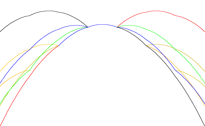
Figure 2. See Example 5.6.

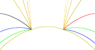
Figure 3. Added detail for part of Figure 2 showing additional continuations near the ends of the original function.

Example 5.6.

This example is related to Examples 3.5 and 3.6. Let $G_{p}$ be the attractor of the affine IFS

$$\mathcal{W}_{p}=(\mathbb{R}^{2},w_{1}(x,y)=(0.5x,0.5x+py),w_{2}(x,y)=(0.5x+1,-0.5x+py+1),$$

where $p\in(-1,0)\cup(0,1)$ is a parameter.

When $p=0.25$ the attractor $G_{0.25}$ is the graph of the analytic function $f\,:[0,2]\rightarrow{\mathbb{R}}$, where

$$f(x)=x(2-x)$$

and, according to statement (3) of Theorem 5.4 the unique continuation is $f_{\theta}(x)=x(2-x)$ with domain $[0,\infty)$ if $\theta=\overline{1}$, domain $(-\infty,2]$ if $\theta=\overline{2}$, and domain $(-\infty,\infty)$ otherwise.

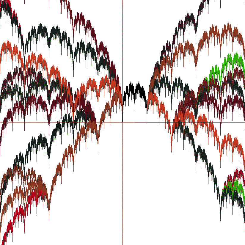
Figure 4. See Example 5.6. The colors help to distinguish the different continuations of the fractal function whose graph is illustrated in black near the center of the image.

When $p=0.3$ the attractor is the graph of a non-differentiable function and there are non-denumerably many distinct continuations $f_{\theta}\,:\,(-\infty,\infty)\rightarrow\mathbb{R}$. Figure 2 shows some of these continuations, restricted to the domain $[-20,20]$. More precisely, Figure 2 shows the graphs of $f_{\theta|4}(x)$ for all $\theta\in\{1,2\}^{\infty}.$ The continuation $f_{\overline{1}}(x)$, on the right in black, coincides exactly, for $x\in[2,4]$, with all continuations of the form $f_{1\rho}(x)$ with $\rho\in\{1,2\}^{\infty}.$ To the right of center: the blue curve is $G_{2111}$, the green curve is $G_{2211}$, and the red curve is $G_{2221}$. On the left: the lowest curve (part red, part blue) is $G_{2222}$, the green curve is $G_{1222}$, the blue curve is $G_{1122}$, and the black curve is $G_{1112}$. Also see Figure 3.

For $p=0.8$ the attractor $G_{0.8}$ is the graph of a fractal function $f_{0.8}$ whose graph has Minkowski dimension $(2-\ln(5/4)/\ln 2)$. This graph $G_{0.8}$ is illustrated in the middle of Figure 4. The window for Figure 4 is $[-10,10]\times[-10,10]\subset\mathbb{R}^{2},$ and $f_{0.8}$ is the (unique) black object whose domain is $[0,2]$. Figure 4 shows all continuations $f_{\theta|4}(x)$ for $\theta\in\{1,2\}^{\infty}.$

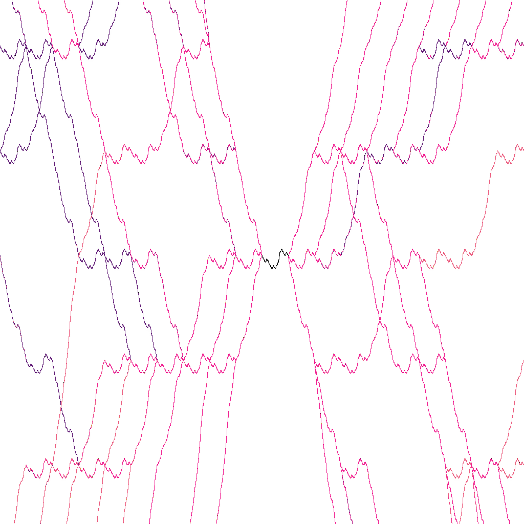
Figure 5. See Example 5.8.

Example 5.7.

(continuation of a nowhere differentiable function of Weierstrasse) We continue Example 3.9. It is readily calculated that, for all $\xi\in[0,1)$,

$$w_{1}^{-1}(x,y)=(2x,\left(y-\sin 2\pi x\right)/\xi),w_{2}^{-1}(x,y)=(2x-1,(y-\sin 2\pi x)/\xi)$$

from which it follows that

$$f_{\theta}(x)=\sum\limits_{k=0}^{\infty}\xi^{k+1}\sin 2^{k+1}\pi x$$

with domain $[0,\infty)$ if $\theta=\overline{1}$, domain $(-\infty,2]$ if $\theta=\overline{2}$, and domain $(-\infty,\infty)$ otherwise. In this example, all continuations agree, where they are defined, both with each other and with unique function defined by periodic extension of equation (9).

When $\mathcal{W}$ in Theorem 5.4 is affine and $M=2$ write, for $n\in\mathcal{I}$,

$$F_{n}(x,y)=c_{n}x+d_{n}y+e_{n}.$$

We refer to the free parameter $d_{n}\in\mathbb{R}$, constrained by $\left|d_{n}\right|<1,$ as a vertical scaling factor. If the verticle scaling factors are fixed and we require that the attractor interpolate the data $\{(x_{i},y_{i})\}_{i=0}^{N}$, then the affine functions $F_{n}$ are completely determined.

Example 5.8.

The IFS $\mathcal{W}$ comprises the four affine maps $w_{n}(x,y)=\linebreak(L_{n}(x),F_{n}(x,y))$ that define the fractal interpolation function $f:[0,1]\rightarrow\mathbb{R}$ specified by the data

$$\{(0,0.25),(0.25,0),(0.5,-0.25),(0.75,0.5),(1,0.25)\},$$

with vertical scaling factor $0.25$ on all four maps. Figure 5 illustrates the attractor, the graph of $f$, together with graphs of all continuations $f_{ijkl}$ where $i,j,k,l\in\{1,2,3,4\}$. The window is $[-10,10]^{2}$.

Example 5.9.

The IFS $\mathcal{W}$ comprises the four affine maps with respective vertical scaling factors $(0.55,0.45,0.45,0.45)$ such that the attractor interpolates the data

$$\{(0,0.25),(0.25,0),(0.5,0.15),(0.75,0.6),(1,0.25)\}.$$

Figure 6 illustrates the attractor, an affine fractal interpolation function $f:[0,1]\rightarrow\mathbb{R}$, together with all continuations $f_{ijkl}$ where $i,j,k,l\in\{1,2,3,4\}$. The window is $[-20,20]^{2}$.

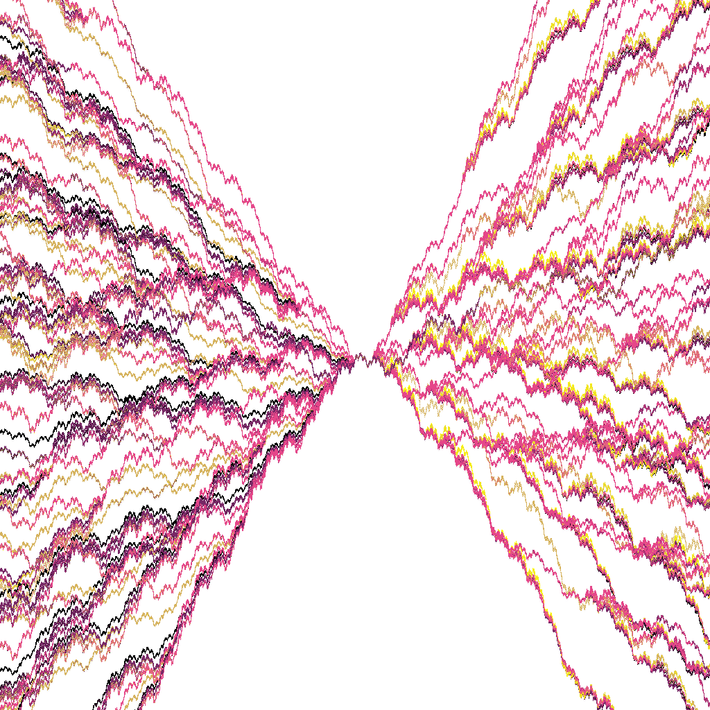
Figure 6. See Example 5.9.

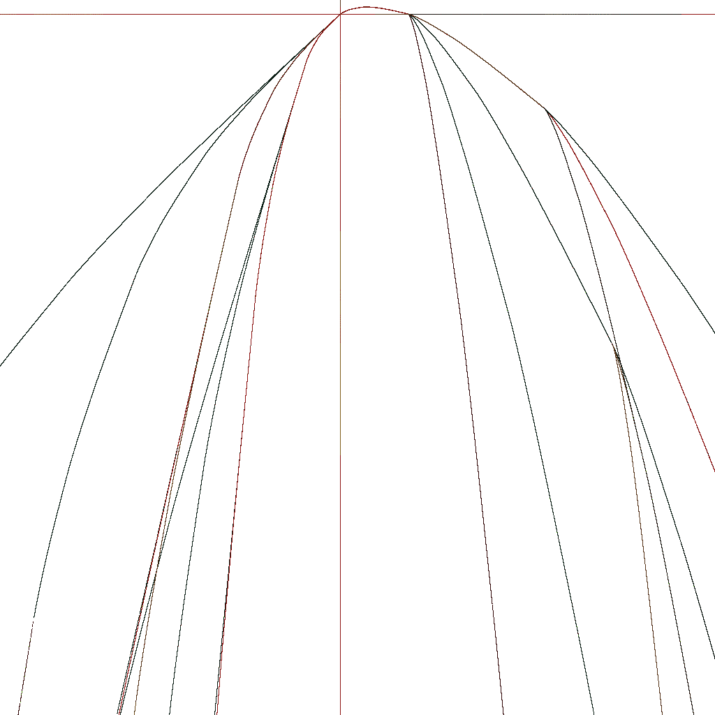
Figure 7. See Example 5.10.

Example 5.10.

Figure 7 shows continuations of the fractal function $f:[0,2]\rightarrow\mathbb{R}$ described in Example 3.7. These are the continuations $f_{ijkl}(x)$ $(ijkl\in\{0,1\}^{4})$. The $x$-axis between $x=-10$ and $x=11$ and $y$-axis between $y=-100$ and $y=2$ are also shown. The graph of $f$ is the part of the image above the $x$-axis.

In order to describes some relationships between the continuations $\{f_{\theta}:\theta\in\mathcal{I}^{\infty}\}$ (see the previous examples), note that, for any finite string $\sigma$ and any $\theta,\theta^{\prime}\in\mathcal{I}^{\infty}$,

$$f_{\sigma\theta}(x)=f_{\sigma\theta^{\prime}}(x)$$

for all $x\in I_{\sigma}$. Consider the example $I=[0,1],\;N=2$, and

$$L_{1}(x)=\frac{1}{2}\,x,\qquad\qquad L_{2}(x)=\frac{1}{2}\,x+\frac{1}{2}.$$

It is easy to determine $I_{\sigma}$ for various finite strings $\sigma$, some of these intervals illustrated in Figure 8. For example, we must have

$$f_{22\theta}(x)=f_{22\theta^{\prime}}(x)$$

for all $x\in I_{22}=[-3,1]$ and for all $\theta,\theta^{\prime}\in\mathcal{I}^{\infty}$, but, as confirmed by examples, it can occur that $f_{212}(x)\neq f_{221}(x)$ for some $x\in I_{212}\cap I_{221}=[-3,3]$.

There is a natural probability measure on the collection of continuations on $\mathcal{I}^{\infty}$ defined by setting $\Pr(\theta_{i}=1)=0.5$ for all $i=1,2,..,$ independently. Then, because many continuations coincide over a given interval, we can estimate probabilities for the values of the continuations. For example, if $N=2$, $I=[0,1],$ and $a_{1}=a_{2}=1/2,$ then

$$\Pr(f_{\theta}(x) =f_{\overline{1}}(x)\,|\,x\in[1,2])\geq 1/2;$$

$$\Pr(f_{\theta}(x) =f_{\overline{21}}(x)\,|\,x\in[1,2])\geq 1/4;$$

$$\Pr(f_{\theta}(x) =f_{\overline{221}}(x)\,|\,x\in[1,2])\geq 1/8;$$

$$\Pr(f_{\theta}(x) =f\underset{n}{{}_{\underbrace{\overline{2...221}}}}(x)\,|\,x\in[1,2])\geq 1/2^{n}\text{ for all }n=1,2,\cdots$$

In this sense, Figures 2, 5, and 7 illustrate probable continuations.

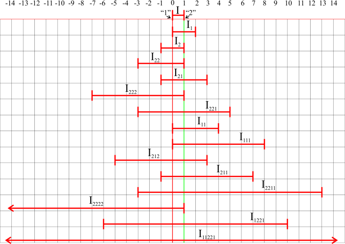
Figure 8. An example of domains of agreements between ss analytic continuations. See the end of Section 5

6. Uniqueness of fractal continuations

This section contains some results concerning the uniqueness of the set of fractal continuations. Our conjecture is that an analytic fractal function $f$ has a unique set of continuations, indpependent of the particular IFS that generates the graph of $f$ as the attractor. More precisely, suppose that $G(f)$, the graph of a continuous function $f:I\rightarrow\mathbb{R}$, is the attractor of an analytic interpolation IFS $\mathcal{W}$ with set of continuations $\{f_{\theta}:\theta\in\mathcal{I}^{\infty}\}$ as defined in Section 5, and the same $G(f)$ is also the attractor of another analytic interpolation IFS $\widetilde{\mathcal{W}}=\{\mathbb{R}^{M};\widetilde{w}_{n},n\in\widetilde{\mathcal{I}}\}$ with set of continuations $\{\widetilde{f}_{\theta}:\theta\in\widetilde{\mathcal{I}}^{\infty}\}$. The conjecture is that the two sets of continuations are equal (although they may be indexed differently). This is clearly true if $f$ is itself analytic, since an analytic function has a unique analytic continuation. In this section we prove that the conjecture is true under certain fairly general conditions when $f$ is not analytic. Recall that the relevant IFSs are of the form

(13 ) $$\mathcal{W} =\left\{\mathbb{X\subset R}^{2};\,w_{n}(x,y)=(L_{n}(x),F_{n}(x,y)),\,n\in{\mathcal{I}}\right\},$$

$$L_{n}(x) =a_{n}x+b_{n}$$

for $n=1,2,\dots,N$. The first result concerns the extensions $f_{\overline{1}}(x)$ and $f_{\overline{N}}(x)$. This is a special case, but introduces some key ideas.

Theorem 6.1.

Let $\mathcal{W}$ and $\widetilde{\mathcal{W}}$ be analytic interpolation IFSs, each with the same attractor $G(f)=G(\widetilde{f})$ but with possibly different numbers, say $N$ and $\widetilde{N}$ of maps. Then

$$f_{\overline{1}}(x)=\widetilde{f}_{\overline{1}}(x)\qquad\text{ and }\qquad f_{\overline{N}}(x)={\widetilde{f}}_{\overline{\widetilde{N}}}(x)$$

for all $x\in\mathbb{R}$ such that $(x,y)\in\mathbb{X}$ for some $y\in\mathbb{R}$.

Proof.

As previously mentioned, it is sufficient to prove the theorem when $f$ is not an analytic function. In this case $f$ must not possess a derivative of some order at some point. By the self-similarity property (2) mentioned in the Introduction, $f$ must possess a dense set of such points. Hence, as a consequence of the Weierstrass preparation theorem [11], if a real analytic function $g(x,y)$ vanishes on $G(f)$, then $g(x,y)$ must be identically zero. Now, since $L_{1}\circ\widetilde{L_{1}}=\widetilde{L_{1}}\circ L_{1}$ it follows, again from the self-similarity property, that $\left(w_{1}\circ\widetilde{w_{1}}\right)(x,y)=\left(\widetilde{w_{1}}\circ w_{1}\right)(x,y)$ for all $(x,y)\in G(f).$ Then

$$g(x,y)=(w_{1}\circ\widetilde{w_{1}}-\widetilde{w_{1}}\circ w_{1})(x,y)$$

vanishes on $G(f)$. Hence $w_{1}\circ\widetilde{w_{1}}=\widetilde{w_{1}}\circ w_{1}$ for all $(x,y)$ in $\mathbb{X}$. It follows, on multiplying on the left by $w_{1}^{-1}$ and on the right by $w_{1}^{-1}$ that

$$w_{1}^{-1}\circ\widetilde{w_{1}}=\widetilde{w_{1}}\circ w_{1}^{-1},$$

and similarly that $w_{1}\circ\widetilde{w_{1}}^{-1}=\widetilde{w_{1}}^{-1}\circ w_{1}$.

Now suppose that $(x,y)\in G(f_{\overline{1}})$. Then $(x,y)\in G(f_{\overline{1|}k})=w_{1}^{-1}\circ...\circ w_{1}^{-1}(G(f))$ for some $k$. Hence we can choose $l$ so large that

$$\begin{array}[]{c}\underbrace{\widetilde{w_{1}}\circ\widetilde{w_{1}}\circ\cdots\widetilde{w_{1}}}\\ l\text{ times}\end{array}(x,y) \in\widetilde{w_{1}}\circ\widetilde{w_{1}}\circ\cdots\widetilde{w_{1}}\circ w_{1}^{-1}\circ...\circ w_{1}^{-1}(G(f))$$

$$\subseteq w_{1}^{-1}\circ\cdots\circ w_{1}^{-1}\begin{array}[]{c}\underbrace{\widetilde{w_{1}}\circ\widetilde{w_{1}}\circ\cdots\widetilde{w_{1}}}\\ l\text{ times}\end{array}(G(f))$$

$$\subset G(f)$$

which implies

$$(x,y)\in\begin{array}[]{c}\underbrace{\widetilde{w_{1}}^{-1}\circ\widetilde{w_{1}}^{-1}\circ....\widetilde{w_{1}}^{-1}}\\ l\text{ times}\end{array}(G(f))$$

when $l$ is sufficiently large. Hence $G(f_{\overline{1}})\subset G(\widetilde{f}_{\overline{\widetilde{1}}})$. The opposite inclusion is proved similarly, as is the result for the other endpoint.    

6.1. Differentiability of fractal functions.

We are going to need the following result, which is interesting in its own right, as it provides detailed information about analytic fractal functions.

Theorem 6.2.

Let $\mathcal{W}$ be an analytic interpolation IFS of the form given in equation (13) with attractor $G(f)$. Let $c\in[0,\infty)$ and $d\in[0,1)$ be real constants such that $\left|\frac{\partial}{\partial x}F_{n}(x,y)\right|<c$ and $0\leq\left|\frac{\partial}{\partial y}F_{n}(x,y)\right|\leq da_{n}$ for all $(x,y)$ in some neighborhood of $G(f)$, for all $n\in\mathcal{I}$. The function $f:[x_{0},x_{N}]\rightarrow\mathbb{R}$ is lipschitz with lipshitz constant $\lambda=a^{-1}c(1-d)^{-1},$ where $a=\min\{a_{n}:n=1,2,...,N\}$. That is:

(14 ) $$\left|f\left(s\right)-f(t)\right|\leq\lambda\,\left|s-t\right|\text{ for all }s,t\in[x_{0},x_{N}].$$

Proof.

Consider the sequence of iterates $k=0,1,2,\dots$

$$f_{k+1}(x)=\left(Wf_{k}\right)(x)=F_{n}(L_{n}^{-1}(x),f_{k}(L_{n}^{-1}(x)))$$

for $x\in[x_{n-1},x_{n}],n=1,2,\dots,N$, where $W$ is as defined in the statement of Theorem 3.2. Without loss of generality, suppose that $\{f_{k}\}$ is contained in the neighborhood $\mathbb{X}$ of $G(f)$ mentioned in the statement of the theorem. It will first be shown, by induction, that $f_{k}$ is lipschitz. Suppose that $f_{k}(x)$ is lipshitz on $[x_{0},x_{N}]$ with constant $\lambda$. Then, for all $s,t\in[x_{n-1},x_{n}],\,n=1,2,...,N$ we have, by the self-replicating property, by the mean value theorem for some $(\varsigma,\zeta)\in\mathbb{X}$, and by the induction hypothesis that

$$\left|f_{k+1}(s)-f_{k+1}(t)\right| =\left|F_{n}(L_{n}^{-1}(s),f_{k}(L_{n}^{-1}(s)))-F_{n}(L_{n}^{-1}(t),f_{k}(L_{n}^{-1}(t)))\right|$$

$$\leq\left|F_{n}(L_{n}^{-1}(s),f_{k}(L_{n}^{-1}(t)))-F_{n}(L_{n}^{-1}(t),f_{k}(L_{n}^{-1}(t)))\right|$$

$$+\left|F_{n}(L_{n}^{-1}(s),f_{k}(L_{n}^{-1}(s)))-F_{n}(L_{n}^{-1}(s),f_{k}(L_{n}^{-1}(t)))\right|$$

$$=\left|L_{n}^{-1}(s)-L_{n}^{-1}(t)\right|\cdot\left|\frac{\partial}{\partial x}F_{n}(x,y)\right|_{(\varsigma,t)}$$

$$+\left|f_{k}(L_{n}^{-1}(s))-f_{k}(L_{n}^{-1}(t)))\right|\cdot\left|\frac{\partial}{\partial y}F_{n}(x,y)\right|_{(s,\zeta)}$$

$$\leq\left(a_{n}^{-1}c+\lambda\,a_{n}^{-1}\,d\right)\left|s-t\right|\leq\left(a^{-1}c+\lambda\,d\right)\left|s-t\right|$$

$$=\left(a^{-1}c+a^{-1}c(1-d)^{-1}\,d\right)\left|s-t\right|=\lambda\,\left|s-t\right|.$$

Now suppose that $s<t$ and $s\in[x_{m-1},x_{m}]$ and $t\in[x_{n-1},x_{n}]$ where $m<n$. Then

$$\left|f_{k+1}(s)-f_{k+1}(t)\right| \leq\left|f_{k+1}(s)-f_{k+1}(x_{m})\right|+\left|f_{k+1}(x_{m})-f_{k+1}(x_{m+1})\right|$$

$$+\dots+\left|f_{k+1}(x_{n})-f_{k+1}(t)\right|$$

$$\leq\lambda\,\left|s-x_{m}\right|+\lambda\,\left|x_{m}-x_{m+1}\right|+\dots+\lambda\,\left|x_{n}-t\right|=\lambda\,\left|s-t\right|.$$

Therefore $f_{k}(x)$ is lipshitz on $[x_{0},x_{N}]$ with constant $\lambda$ for all $k$.

Now we use the fact that $\left\{f_{k}\right\}$ converges uniformly to $f$ on $[x_{0},x_{N}]$, specifically

$$\max\{|f(x)-f_{k}(x)|:x\in[x_{0},x_{N}]\} =\max\{|W^{k}f(x)-W^{k}f_{0}(x)|:x\in[x_{0},x_{N}]\}$$

$$\leq s^{k}\,\max\{|f(x)-f_{0}(x)|:x\in[x_{0},x_{N}]\}$$

for $s$ as in the proof of Theorem 3.2. The unform limit of a sequence of functions with lipschitz constant $\lambda$ is a lipshitz function with constant $\lambda$.    

For an interpolation IFS $\mathcal{W}$ of the form given in equation (13) with attractor $G(f)$, consider the IFS

$$\mathcal{L}:\mathcal{=\{}I=[x_{0},x_{N}];\,L_{n}(x)=a_{n}x+b_{n},n\in\mathcal{I}\},$$

and let

$$\mathcal{D}_{\mathcal{L}} =\bigcup\limits_{k=0}^{\infty}\mathcal{L}^{k}(\{x_{0},x_{1},\dots,x_{N}\})\backslash\{x_{0},x_{N}\},$$

$${\mathcal{D}}_{\mathcal{W}} =\{(x,f(x))\,:\,x\in{\mathcal{D}}_{\mathcal{L}}\}.$$

The set ${\mathcal{D}}_{\mathcal{W}}$ will be referred to as the set of double points of $G(f)$. The standard method for addressing the points of the attractor of a contractive IFS [2] can be applied to draw the following conclusions. If $(x,y)$ is a point of $G(f)$ that is not a double point, then there is a unique $\sigma\in{\mathcal{I}}^{\infty}$ such that

$$x =\lim_{k\rightarrow\infty}L_{\sigma|k}(s),$$

$$(x,y) =\lim_{k\rightarrow\infty}w_{\sigma|k}(s,t),$$

where the limit is independent of $(s,t)\in\mathbb{X}$. If $(x,y)$ is a double point, then there exist two distinct strings $\sigma$ such that the above equations hold. In any case, we use the notation $\pi\,:\,{\mathcal{I}}^{\infty}\rightarrow{\mathbb{R}}$,

$$\pi(\sigma):=\lim_{k\rightarrow\infty}L_{\sigma|k}(s),$$

which is independent of $s\in\mathbb{R}$.

Theorem 6.3.

Let $\mathcal{W}$ be an analytic interpolation IFS of the form given in equation (13) with attractor $G(f)$ and such that $0<\left|\partial F_{n}(x,y)/\partial y\right|<a_{n}$ for all $(x,y)\in\mathbb{X}$ and for all $n\in\mathcal{I}$. If $x$ is not a double point of $G(f)$, then $f$ is differentiable at $x$.

Proof.

For now, fix $k\in\mathbb{N}.$ Define the function $Q:\mathbb{R}^{k+1}\rightarrow\mathbb{R}$ by

$$Q(x_{1},x_{2},\dots,x_{k},y)=F_{\sigma_{1}}(x_{1},F_{\sigma_{2}}(x_{2},\dots F_{\sigma_{k}}(x_{k},y)\dots)).$$

where the domain of $Q$ is all $(x_{1},x_{2},\dots,x_{k},y)$ such that $(x_{j},y)\in\mathbb{X}$ for all $j=1,2,\dots,k.$ Let

$$H_{n}(x,y):=\frac{\partial}{\partial x}F_{n}(x,y),\qquad\qquad K_{n}(x,y):=\frac{\partial}{\partial y}F_{n}(x,y)$$

for $n\in\mathcal{I}$. Because $F_{n}(x,y)$ is analytic for each $n$, there are constants $c\in[0,\infty)$ and $d_{n}\in[0,a_{n})$ such that

(15 ) $$\left|H_{n}(x,y)\right|\leq c,\qquad\qquad\left|K_{n}(x,y)\right|<d_{n}$$

for all $n\in\mathcal{I}$ and for all $(x,y)$ in some neighborhood of $G(f)$. Using the notation

$$Q_{x_{l}}(x_{1},x_{2},\dots,x_{k},y) :=\frac{\partial}{\partial x_{l}}Q(x_{1},x_{2},\dots,x_{k},y)$$

$$Q_{y}(x_{1},x_{2},\dots,x_{k},y) :=\frac{\partial}{\partial y}Q(x_{1},x_{2},\dots,x_{k},y),$$

we have the following for $l=1,2,\dots,k$:

$$Q_{x_{l}}(x_{1},x_{2},\dots,x_{k},y) =K_{\sigma_{1}}(x_{1},F_{\sigma_{2}}(x_{2},\dots F_{\sigma_{k}}(x_{k},y)\dots))\cdot K_{\sigma_{2}}(x_{2},F_{\sigma_{3}}(x_{3},\dots F_{\sigma_{k}}(x_{k},y)\dots))\cdot\dots$$

$$K_{\sigma_{l-1}}(x_{l-1},\dots F_{\sigma_{k}}(x_{k},y)\dots))\cdot H_{\sigma_{l}}(x_{l},F_{\sigma_{l\mathfrak{+1}}}(x_{l+1},\dots F_{\sigma_{k}}(x_{k},y)\dots));$$

$$Q_{y}(x_{1},x_{2},\dots,x_{k},y) =K_{\sigma_{1}}(x_{1},F_{\sigma_{2}}(x_{2},\dots F_{\sigma_{k}}(x_{k},y)\dots))\cdot K_{\sigma_{2}}(x_{2},F_{\sigma_{3}}(x_{3},\dots F_{\sigma_{k}}(x_{k},y)\dots))\cdot\dots$$

$$K_{\sigma_{k-1}}(x_{k-1},F_{\sigma_{k}}(x_{k},y))\cdot K_{\sigma_{k}}(x_{k},y).$$

Using the intermediate value theorem repeatedly we have, for some $\eta_{l}\in[x_{l},x_{l}+\delta x_{l}]$, $l=1,2,\dots,k$, and $\xi\in[y,y+\delta y]$:

$$\Delta Q:= \,Q(x_{1}+\delta x_{1},x_{2}+\delta x_{2},\dots,x_{k}+\delta x_{k},y+\delta y)-Q(x_{1},x_{2},\dots,x_{k},y)$$

$$= \,[Q(x_{1}+\delta x_{1},x_{2}+\delta x_{2},\dots,x_{k}+\delta x_{k},y+\delta y)-Q(x_{1},x_{2}+\delta x_{2},\dots,x_{k}+\delta x_{k},y+\delta y)]+$$

$$[Q(x_{1},x_{2}+\delta x_{2},\dots,x_{k}+\delta x_{k},y+\delta y)-Q(x_{1},x_{2},x_{3}+\delta x_{3},\dots,x_{k}+\delta x_{k},y+\delta y)]+\dots$$

$$[Q(x_{1},x_{2},\dots x_{k-1},x_{k}+\delta x_{k},y+\delta y)-Q(x_{1},x_{2},\dots,x_{k},y+\delta y)]+$$

$$[Q(x_{1},x_{2},\dots,x_{k},y+\delta y)-Q(x_{1},x_{2},\dots,x_{k},y)]$$

$$= \,Q_{x_{1}}(\eta_{1},x_{2}+\delta x_{2},\dots,x_{k}+\delta x_{k},y+\delta y)\delta x_{1}+$$

$$Q_{x_{2}}(x_{1},\eta_{2},x_{3}+\delta x_{3}\dots,x_{k}+\delta x_{k},y+\delta y)\delta x_{2}+\dots+$$

$$Q_{x_{k}}(x_{1},x_{2},x_{3}\dots x_{k-1},\eta_{k},y+\delta y)\delta x_{k}+$$

$$Q_{y}(x_{1},x_{2},x_{3}\dots,x_{k},\xi)\delta y\text{.}$$

Let $\sigma=\pi^{-1}(x)$, which is well defined since $x$ is not a double point, and $x_{j}=\left(L_{\sigma|j}\right)^{-1}(x).$ By the self-repicating property (3)

$$f_{k}(x)=F_{\sigma_{1}}(x_{1},F_{\sigma_{2}}(x_{2},\dots F_{\sigma_{k}}(x_{k},f_{0}(x_{k}))\dots)).$$

Fix $k$ and $\sigma$ and let both $x$ and $(x+\delta x)$ lie in $L_{\sigma|k}([0,1])$. Define

$$\begin{aligned} x_{j}&=\left(L_{\sigma|j}\right)^{-1}(x)\\ y&=f((L_{\sigma|k})^{-1}(x))\end{aligned}\qquad\begin{aligned} x_{j}+\delta x_{j}&=(L_{\sigma|j})^{-1}(x+\delta x)=(L_{\sigma|j})^{-1}(x)+(a_{\sigma_{1}}\dots a_{\sigma_{j}})^{-1}\delta x\\ y+\delta y&=f((L_{\sigma|k})^{-1}(x+\delta x)).\end{aligned}$$

Then

$$[f(x+\delta x)-f(x)]/\delta x$$

$$=[F_{\sigma_{1}}(x_{1}+\delta x_{1},F_{\sigma_{2}}(x_{2}+\delta x_{2},\dots F_{\sigma_{k}}(x_{k}+\delta x_{k},y+\delta y)\dots))-$$

$$\hskip 14.22636ptF_{\sigma_{1}}(x_{1},F_{\sigma_{2}}(x_{2},\dots F_{\sigma_{k}}(x_{k},y)\dots))]/\delta x$$

$$=\Delta Q/\delta x$$

$$=[Q_{x_{1}}(\eta_{1},x_{2}+\delta x_{2},\dots,x_{k}+\delta x_{k},y+\delta y)\cdot(a_{\sigma_{1}})^{-1}+$$

$$\hskip 14.22636ptQ_{x_{2}}(x_{1},\eta_{2},x_{3}+\delta x_{3}\dots,x_{k}+\delta x_{k},y+\delta y)\cdot(a_{\sigma_{1}}a_{\sigma_{2}})^{-1}+\dots$$

$$\hskip 14.22636ptQ_{x_{k}}(x_{1},x_{2},x_{3}\dots x_{k-1},\eta_{k},y+\delta y)\cdot(a_{\sigma_{1}}\dots a_{\sigma_{k}})^{-1}]+$$

$$\hskip 14.22636ptQ_{y}(x_{1},x_{2},x_{3}\dots,x_{k},\xi)\cdot(a_{\sigma_{1}}\dots a_{\sigma_{k}})^{-1}\cdot$$

$$\hskip 22.76219pt\left[f(\left(L_{\sigma|k}\right)^{-1}(x)+((a_{\sigma_{1}}\dots a_{\sigma_{k}})^{-1}\cdot\delta x)-f(\left(L_{\sigma|k}\right)^{-1}(x))\right]/((a_{\sigma_{1}}\dots a_{\sigma_{k}})^{-1}\cdot\delta x)$$

and

$$[f(x+\delta x)-f(x)]/\delta x$$

$$=[c_{1}a_{\sigma_{1}}^{-1}+c_{2}d_{2,1}a_{\sigma_{1}}^{-1}a_{\sigma_{2}}^{-1}+c_{3}d_{3,1}d_{3,2}a_{\sigma_{1}}^{-1}a_{\sigma_{2}}^{-1}a_{\sigma_{3}}^{-1}+\dots$$

$$\hskip 14.22636pt+c_{k}d_{k,1}d_{k,2}\dots d_{k,\left(k-1\right)}(a_{\sigma_{1}}\dots a_{\sigma_{k}})^{-1}]$$

$$=\frac{c_{1}}{a_{\sigma_{1}}}+\frac{c_{2}}{a_{\sigma_{1}}}\frac{d_{2,1}}{a_{\sigma_{2}}}+\dots\frac{c_{2}}{a_{\sigma_{1}}}\frac{d_{3,1}d_{3,2}}{a_{\sigma_{2}}a_{\sigma_{3}}}+\dots\frac{c_{k}}{a_{\sigma_{1}}}\frac{d_{k,1}d_{k,2}\dots d_{k,\left(k-1\right)}}{a_{\sigma_{2}}a_{\sigma_{3}}\dots a_{\sigma_{k}}}$$

$$\hskip 14.22636pt+\frac{Q_{y}(x_{1},x_{2},x_{3}\dots,x_{k},\xi)}{a_{\sigma_{1}}a_{\sigma_{2}}a_{\sigma_{3}}\dots a_{\sigma_{k}}}\left[\frac{f((L_{\sigma|k})^{-1}(x+\delta x))-f((L_{\sigma|k})^{-1}(x))}{(L_{\sigma|k})^{-1}(x+\delta x)-(L_{\sigma|k})^{-1}(x)}\right]$$

where

$$c_{1} =H_{\sigma_{1}}(\eta_{1},F_{\sigma_{2}}(x_{2}+\delta x_{2},\dots F_{\sigma_{k}}(x_{k}+\delta x_{k},y+\delta y)\dots)),$$

$$c_{2} =H_{\sigma_{2}}(\eta_{2},F_{\sigma_{3}}(x_{3}+\delta x_{3},\dots F_{\sigma_{k}}(x_{k}+\delta x_{k},y+\delta y)\dots)),$$

$$\ddots$$

$$c_{k} =H_{\sigma_{k}}(\eta_{k},y+\delta y),$$

and

$$d_{2,1} =K_{\sigma_{1}}(x_{1},F_{\sigma_{2}}(\eta_{2},F_{\sigma_{3}}(x_{3}+\delta x_{3},\dots F_{\sigma_{k}}(x_{k}+\delta x_{k},y)\dots)))$$

$$d_{3,1} =K_{\sigma_{1}}(x_{1},F_{\sigma_{2}}(x_{2},F_{\sigma_{3}}(\eta_{3},F_{\sigma_{3}}(x_{4}+\delta x_{4},\dots F_{\sigma_{k}}(x_{k}+\delta x_{k},y)\dots))))$$

$$d_{3,2} =K_{\sigma_{2}}(x_{2},F_{\sigma_{3}}(\eta_{3},F_{\sigma_{4}}(x_{4}+\delta x_{4},\dots F_{\sigma_{k}}(x_{k}+\delta x_{k},y)\dots)))$$

$$\ddots$$

$$d_{l,1} =K_{\sigma_{1}}(x_{1},F_{\sigma_{2}}(x_{2},\dots F_{\sigma_{l-1}}(x_{l-1},F_{\sigma_{l}}(\eta_{l},F_{\sigma_{l+1}}(x_{l+1}+\delta x_{l+1},\dots F_{\sigma_{k}}(x_{k}+\delta x_{k},y)\dots))))$$

$$d_{l,2} =K_{\sigma_{2}}(x_{2},F_{\sigma_{2}}(x_{2},\dots F_{\sigma_{l-1}}(x_{l-1},F_{\sigma_{l}}(\eta_{l},F_{\sigma_{l+1}}(x_{l+1}+\delta x_{l+1},\dots F_{\sigma_{k}}(x_{k}+\delta x_{k},y)\dots)))))$$

$$\ddots$$

$$d_{l,l-1} =F_{\sigma_{l-1}}(x_{l-1},F_{\sigma_{l}}(\eta_{l},F_{\sigma_{l+1}}(x_{l+1}+\delta x_{l+1},\dots F_{\sigma_{k}}(x_{k}+\delta x_{k},y)\dots)))$$

$$d_{k,1} =K_{\sigma_{1}}(x_{1},F_{\sigma_{2}}(x_{2},\dots F_{\sigma_{l-1}}(x_{l-1},F_{\sigma_{l}}(x_{l},F_{\sigma_{l+1}}(x_{l+1},\dots F_{\sigma_{k}}(\eta_{k},y)\dots))))$$

$$\ddots$$

$$d_{k,k-1} =K_{\sigma_{k-1}}(x_{k-1},F_{\sigma_{k}}(\eta_{k},y)).$$

Note that the $c_{l}$ and $d_{l,m}$ depend explicitly on $k$ (which so far is fixed). It follows that

$$\left|\frac{f(x+\delta x)-f(x)}{\delta x}-\left(\frac{c_{1}}{a_{\sigma_{1}}}+\frac{d_{2,1}}{a_{\sigma_{1}}}\frac{c_{2}}{a_{\sigma_{2}}}+\frac{d_{3,1}d_{3,2}}{a_{\sigma_{1}}a_{\sigma_{2}}}\frac{c_{3}}{a_{\sigma_{3}}}+\cdots+\frac{d_{k,1}d_{k,2}\dots d_{k,\left(k-1\right)}}{a_{\sigma_{1}}a_{\sigma_{2}}\dots a_{\sigma_{k-1}}}\frac{c_{k}}{a_{\sigma_{k}}}\right)\right|$$

$$\leq\left|\frac{Q_{y}(x_{1},x_{2},x_{3}\dots,x_{k},\xi)}{a_{\sigma_{1}}a_{\sigma_{2}}a_{\sigma_{3}}\dots a_{\sigma_{k}}}\right|\cdot\left|\frac{f(S_{k}(x+\delta x))-f(S_{k}(x))}{S^{k}(x+\delta x)-S_{k}(x)}\right|$$

$$\leq\lambda\,\left|\frac{Q_{y}(x_{1},x_{2},x_{3}\dots,x_{k},\xi)}{a_{\sigma_{1}}a_{\sigma_{2}}a_{\sigma_{3}}\dots a_{\sigma_{k}}}\right|,$$

the last inequality by Theorem 6.2. The above is true for all $x,\left(x+\delta x\right)\in[x_{0},x_{N}],\linebreak\delta x\neq 0,k\in\mathbb{N}$. We also have

$$\left|\frac{Q_{y}(x_{1},x_{2},x_{3}\dots,x_{k},\xi)}{a_{\sigma_{1}}a_{\sigma_{2}}a_{\sigma_{3}}\dots a_{\sigma_{k}}}\right| =\frac{\left|K_{\sigma_{1}}(x_{1},F_{\sigma_{2}}(x_{2},\dots F_{\sigma_{k}}(x_{k},\xi)\dots))\right|}{a_{\sigma_{1}}}\cdot$$

$$\frac{\left|K_{\sigma_{2}}(x_{2},F_{\sigma_{3}}(x_{3},\dots F_{\sigma_{k}}(x_{k},\xi)\dots))\right|}{a_{\sigma_{2}}}\cdots$$

$$\frac{\left|K_{\sigma_{k-1}}(x_{k-1},F_{\sigma_{k}}(x_{k},\xi))\right|}{a_{\sigma_{k-1}}}\cdot\frac{\left|K_{\sigma_{k}}(x_{k},\xi)\right|}{a_{\sigma_{k}}}$$

$$\leq\prod\limits_{j=1}^{k}\frac{d_{\sigma_{j}}}{a_{\sigma_{j}}}\leq C^{k}$$

for some $C\in[0,1)$, the last inequality by equation (15). Hence, for any $\varepsilon>0$, we can choose $k$ so large that

(16 ) $$\left|\frac{f(x+\delta x)-f(x)}{\delta x}-\sum\limits_{m=1}^{k}\frac{c_{m}}{a_{\sigma_{m}}}\prod\limits_{l=1}^{m-1}\frac{d_{k,l}}{a_{\sigma_{l}}}\right|<\varepsilon/3\text{.}$$

Note that, by their definitions, for fixed $x$, the $c_{m}$s and $d_{k,l}$s depend upon both $k$ and $\delta x$. Our next goal is to remove the dependence on both $k$ and $\delta x$. For all $l$ and all $k\geq l$ define

(17 ) $$C_{\sigma_{l}} :=H_{\sigma_{l}}(x_{l},f(x_{l})=H_{\sigma_{l}}(x_{l},F_{\sigma_{l+1}}(x_{l+1},\dots F_{\sigma_{k}}(x_{k},f(x_{k}))\dots))$$

$$D_{\sigma_{l}} :=K_{\sigma_{l}}(x_{l},f(x_{l})=K_{\sigma_{l}}(x_{l},F_{\sigma_{l+1}}(x_{l+1},\dots F_{\sigma_{k}}(x_{k},f(x_{k}))\dots)).$$

We are going to show that, for all $\varepsilon>0$ and for $\delta x$ sufficiently small,

(18 ) $$\left|\sum\limits_{m=1}^{k}\frac{C_{{}_{\sigma_{m}}}}{a_{\sigma_{m}}}\prod\limits_{l=1}^{m-1}\frac{D_{\sigma_{l}}}{a_{\sigma_{l}}}-\sum\limits_{m=1}^{k}\frac{c_{m}}{a_{\sigma_{m}}}\prod\limits_{l=1}^{m-1}\frac{d_{k,l}}{a_{\sigma_{l}}}\right|<\varepsilon/3\text{,}$$

and that

(19 ) $$\left|\sum\limits_{m=1}^{\infty}\frac{C_{\sigma_{m}}}{a_{\sigma_{m}}}\prod\limits_{l=1}^{m-1}\frac{D_{\sigma_{l}}}{a_{\sigma_{l}}}-\sum\limits_{m=1}^{k}\frac{C_{\sigma_{m}}}{a_{\sigma_{m}}}\prod\limits_{l=1}^{m-1}\frac{D_{\sigma_{l}}}{a_{\sigma_{l}}}\right|<\varepsilon/3\text{,}$$

which taken together with inequality (16) imply

(20 ) $$\left|\frac{f(x+\delta x)-f(x)}{\delta x}-\sum\limits_{m=1}^{\infty}\frac{C_{\sigma_{m}}}{a_{\sigma_{m}}}\prod\limits_{l=1}^{m-1}\frac{D_{\sigma_{l}}}{a_{\sigma_{l}}}\right|<\varepsilon\text{.}$$

For $|\delta x|$ sufficiently small

$$\left|\sum\limits_{m=1}^{k}\frac{C_{\sigma_{m}}}{a_{\sigma_{m}}}\prod\limits_{l=1}^{m-1}\frac{D_{\sigma_{l}}}{a_{\sigma_{l}}}-\sum\limits_{m=1}^{k}\frac{c_{m}}{a_{\sigma_{m}}}\prod\limits_{l=1}^{m-1}\frac{d_{k,l}}{a_{\sigma_{l}}}\right|$$

$$\leq\sum\limits_{m=1}^{k}\frac{\left|C_{\sigma_{m}}-c_{m}\right|}{a_{\sigma_{m}}}\prod\limits_{l=1}^{m-1}\frac{\left|D_{\sigma_{l}}\right|}{a_{\sigma_{l}}}+\sum\limits_{m=1}^{k}\frac{\left|c_{m}\right|}{a_{\sigma_{m}}}\prod\limits_{l=1}^{m-1}\frac{\left|D_{\sigma_{l}}-d_{k,l}\right|}{a_{\sigma_{l}}}<\varepsilon/3.$$

The last inequality above follow from, for fixed $k,$ the continuous dependence of the $c_{m}$s and $d_{k,l}$s on their independent variables, and comparing $C_{\sigma_{m}}$ with $c_{m}$ and $D_{\sigma_{l}}$ with $d_{k,l}$ using the equalities (17). (We need $|\delta x|$ small enough that $x+\delta x$ lies in $L_{\sigma|k}([0,1])$.) We have established (18). Concerning inequality (19), by equation (15) the $c_{m}$’s are uniformly bounded and, for some $(x,y)$, we have $\left|d_{k,l}\right|=|K_{\sigma_{l}}(x,y)|\leq d_{\sigma_{l}}<a_{\sigma_{l}}$. Therefore $|d_{k,l}/a_{\sigma_{l}}|\leq|d_{\sigma_{l}}/a_{\sigma_{l}}|\leq K$ for some constant $K<1$. So inequality (19) follows from the absolute convergence of the series $\sum\limits_{m=1}^{\infty}\frac{C_{\sigma_{m}}}{a_{\sigma_{m}}}\prod\limits_{l=1}^{m-1}\frac{D_{\sigma_{l}}}{a_{\sigma_{l}}}$. From Equation (20) it follows that

$$f^{\prime}(x)=\sum\limits_{m=1}^{k}\frac{C_{{}_{\sigma_{m}}}}{a_{\sigma_{m}}}\prod\limits_{l=1}^{m-1}\frac{D_{\sigma_{l}}}{a_{\sigma_{l}}}.$$

   

Note that the last equality in the above proof actually provides a formula for the derivative at each point that is not a double point.

6.2. Unicity Theorem

We conjecture that the uniqueness of the set of continuations holds in general. The following theorem provides a proof in ${\mathbb{R}}^{2}$ under the assumption that the derivative $f^{\prime}(x)$ does not exist at all points $x$, although we conjecture that uniqueness holds in ${\mathbb{R}}^{M},M\geq 2$, and it is sufficient to assume that $f(x)$ is not analytic. It is also assumed that there is a bound $\left|\partial F_{n}(x,y)/\partial y\right|<a_{n}$, where the $a_{n}$ are as given in equation (13). As an example, consider the case of affne fractal interpolation functions, where $F_{n}(x,y)=(a_{n}x+b_{n},c_{n}x+d_{n}y+g_{n})$. Then for Theorem 6.4 to apply we need $\left|d_{n}\right|<a_{n}$ for all $n$.

Theorem 6.4.

Let $\mathcal{W}=\{\mathbb{X\subset R}^{2};\,w_{n}(x,y)=(L_{n}(x),F_{n}(x,y)),\,n\in\mathcal{I}\}$ and $\widetilde{\mathcal{W}}=\{\mathbb{X\subset R}^{2};\,\widetilde{w}_{n}(x,y))=(\widetilde{L}_{n}(x),\widetilde{F}_{n}(x,y)),\,n\in\mathcal{I}\}$ be analytic interpolation IFSs as in equation (13) such that $0<\left|\partial F_{n}(x,y)/\partial y\right|<a_{n}$ and $0<\left|\partial\widetilde{F}_{n}(x,y)/\partial y\right|<\widetilde{a}_{n}$ for all $(x,y)\in\mathbb{X}$, for all $n\in\mathcal{I}$. If both $\mathcal{W}$ and $\widetilde{\mathcal{W}}$ have the same attractor $G(f)$ such that $f^{\prime}(x)$ does not exist at $x=x_{n},$ for all $n=0,1,2,\dots,N$, then $\mathcal{W=}\widetilde{\mathcal{W}}$.

Proof.

For simplicity we restrict the proof to the case $N=2$. The proof of the result for arbitrary many interpolation points is similar.

We first prove that the set of double points of $G(f)$ with repect to $\widetilde{\mathcal{W}}$ is the same as the set of double points of $\mathcal{W}$. The interpolation points for $\mathcal{W}$ are $\{0,x_{1},1\}$ and the interpolation points for $\widetilde{\mathcal{W}}$ are $\{0,\widetilde{x}_{1},1\}$. By Theorem 6.3 $f(x)$ is differentiable at all points that are not double points with respect to $\mathcal{W}$ and also at all points that are not double points with respect to $\widetilde{\mathcal{W}}$. Moreover, $f(x)$ is not differentiable at all double points with respect to $\mathcal{W}$ and also not differentiable at all points which are double points with respect to $\widetilde{\mathcal{W}}$. (Otherwise $f(x)$ must be differentiable at $x_{1}$ which would imply that $f(x)$ is differentiable everywhere, contrary to the assumptions of the theorem.) It follows that $f(x)$ is not differentiable at $x$ if and only if $x$ is a double points with respect to $\mathcal{W}$ if and only if $x$ is a double point with respect to $\widetilde{\mathcal{W}}$.

We next prove that $w_{n}(x,y)=\widetilde{w}_{n}(x,y)$ for all $(x,y)\in G(f)$ and $n=1,2,\dots,N$. Since $\widetilde{x}_{1}$ is a double point of $G(f)$ with respect to $\mathcal{W}$ there must be $\sigma|k\neq\emptyset$ such that $w_{\sigma|k}(x_{1},f(x_{1}))=(\widetilde{x}_{1},f(\widetilde{x}_{1}))$. Since $x_{1}$ is a double point of $G(f)$ with respect to $\widetilde{\mathcal{W}}$ there must be $\widetilde{\sigma}|\widetilde{k}$ such that ${\widetilde{w}}_{\widetilde{\sigma}|\widetilde{k}}(\widetilde{x}_{1},f(\widetilde{x}_{1}))=(x_{1},f(x_{1}))$. It follows that ${\widetilde{w}}_{(\widetilde{\sigma}|\widetilde{k})}(w_{(\sigma|k)}(x_{1},f(x_{1})))=(x_{1},f(x_{1}).$ Since $\widetilde{w}_{(\widetilde{\sigma}|\widetilde{k})}\circ w_{(\sigma|k)}:G(f)\rightarrow G(f)$, we can write $\widetilde{w}_{(\widetilde{\sigma}|\widetilde{k})}\circ w_{(\sigma|k)}(x,y)=\overline{w}(x,y)=(\overline{L}(x),\overline{F}(x,y))$ where, similar in form to the functions $\widetilde{w}_{\widetilde{n}}(x,y)$ and $w_{n}(x,y)$ that comprise the two IFSs, $\overline{L}(x)=\overline{a}x+\overline{h}$ is a real affine contraction and $\overline{F}(x,y)$ is analytic in a neighborhood of $G(f)$ and has the property, by the chain rule, that $\left|\frac{\partial\overline{F}}{\partial y}(x,y)\}\right|<\overline{a}$ in a neighborhood of $G(f)$. It is also the case that $\overline{a}x_{1}+\overline{h}=x_{1}$ and $\overline{F}({\overline{L}}^{-1}(x),f({\overline{L}}^{-1}(x)))=f(x)$ in a neighborhood of $x_{1}$ and ${\overline{L}}(x_{1})=x_{1},\;\overline{F}(x_{1},f(x_{1}))=f(x_{1})$. Using the analyticity of $F(x,y)$ in $x$ and $y$,

$$\frac{f(x_{1}+\delta x)-f(x_{1})}{\delta x} =\frac{\overline{F}(L^{-1}(x_{1}+\delta x),f(L^{-1}(x_{1}+\delta x)))-\overline{F}(L^{-1}(x_{1}),f(L^{-1}(x_{1})))}{\delta x}$$

$$=\overline{F}_{x}(x_{1},f(x_{1}))\overline{a}^{-1}$$

$$+\overline{F}_{y}(x_{1},f(x_{1}))\overline{a}^{-1}\frac{\left(f(x_{1}+\overline{a}^{-1}\delta x)-f(x_{1})\right)}{\overline{a}^{-1}\delta x}+o(\delta x).$$

This implies that the following limit exists:

$$\lim_{\delta x\rightarrow 0}\left\{\frac{f(x_{1}+\delta x)-f(x_{1})}{\delta x}-\overline{F}_{y}(x_{1},f(x_{1}))\overline{a}^{-1}\frac{\left(f(x_{1}+\overline{a}^{-1}\delta x)-f(x_{1})\right)}{\overline{a}^{-1}\delta x}\right\}$$

$$=(1-\overline{F}_{y}(x_{1},f(x_{1}))\overline{a}^{-1})f^{\prime}(x_{1})=\overline{F}_{x}(x_{1},f(x_{1}))\overline{a}^{-1},$$

which implies

$$f^{\prime}(x_{1})=\frac{\overline{F}_{x}(x_{1},f(x_{1}))}{(\overline{a}-\overline{F}_{y}(x_{1},f(x_{1})))}.$$

We have shown that if $\sigma|k\neq\emptyset$ then $f(x)$ is differentiable at $x_{1}$, which is not true. Therefore $\sigma|k=\emptyset$ which implies $x_{1}=\widetilde{x}_{1}$ and hence $w_{n}(x,y)=\widetilde{w}_{n}(x,y)$ for a dense set of points $(x,y)$ on $G(f)$. It follows that $w_{n}(x,y)=\widetilde{w}_{n}(x,y)$ for all $(x,y)\in G(f)$ and $n=1,2.$

To show that $\mathcal{W=}\widetilde{\mathcal{W}}$, i.e., that $w_{n}(x,y)-\widetilde{w}_{n}(x,y)$ for all $(x,y)\in\mathbb{X}$, define an analytic function of two variables, $a:\mathbb{X\rightarrow R}$ by $a(x,y):=w_{n}(x,y)-\widetilde{w}_{n}(x,y)$ for all $(x,y)\in\mathbb{X}$. It was shown above that $a(x,y)=0$ for all $(x,y)\in G(f)$. That $a(x,y)=0$ for all $(x,y)\in\mathbb{X}$ follows from the Weierstass preparation theorem [10].    

AKNOWLEDGEMENT

We thank Louisa Barnsley for help with the illustrations.

References

- [1] M. F. Barnsley, Fractal functions and interpolation, Constr. Approx. 2 (1986) 303-329.
- [2] M. F. Barnsley, Fractals Everywhere, Academic Press, 1988; 2nd Edition, Morgan Kaufmann 1993; 3rd Edition, Dover Publications, 2012.
- [3] M. F. Barnsley and A. N. Harrington, The calculus of fractal interpolation functions, Journal of Approximation Theory 57 (1989) 14-34.
- [4] M. F. Barnsley, U. Freiberg, Fractal transformations of harmonic functions, Proc. SPIE 6417 (2006).
- [5] M.A. Berger, Random affine iterated function systems: curve generation and wavelets, SIAM Review 34 (1992) 361-385.
- [6] D.H. Bailey, J.M. Borwein, N.J. Calkin, R. Girgensohn, D.R. Luke, V.H. Moll, Experimental Mathematics in Action, A.K. Peters, 2006.
- [7] J. E. Hutchinson, Fractals and self-similarity, Indiana Univ. Math. J. 30 (1981) 713–747.
- [8] Peter Massopust, Fractal Functions, Fractal Surfaces, and Wavelets, Academic Press, New York, 1995.
- [9] Peter Massopust, Interpolation and Approximation with Splines and Fractals, Oxford University Press, Oxford, New York, 2010.
- [10] R. Narasimhan, Introduction to the theory of analytic spaces, Lecture Notes in Mathematics, volume 25, Springer, 1966.
- [11] M. A. Navascues, Fractal polynomial interpolation, Zeitschrift für Analysis u. i. Anwend, 24 (2005) 401-414.
- [12] Srijanani Anurag Prasad, Some Aspects of Coalescence and Superfractal Interpolation, Ph.D Thesis, Department of Mathematics and Statistics, Indian Institute of Technology, Kanpur, March 2011.
- [13] Robert Scealy, -variable fractals and interpolation, Ph.D. Thesis, Australian National University, 2008
- [14] Eric Tosan, Eric Guerin, Atilla Baskurt, Design and reconstruction of fractal surfaces. In IEEE Computer Society, editor, 6th International Conference on Information Visualisation IV 2002, London, UK pp. 311-316, July 2002.
- [15] Claude Tricot, Curves and Fractal Dimension, Springer-Verlag, New York, 1995.