Improved Asteroid Astrometry and Photometry
with Trail Fitting

Abstract

Asteroid detections in astronomical images may appear as trails due to a combination of their apparent rate of motion and exposure duration. Nearby asteroids in particular typically have high apparent rates of motion and acceleration. Their recovery, especially on their discovery apparition, depends upon obtaining good astrometry from the trailed detections. We present an analytic function describing a trailed detection under the assumption of a Gaussian point spread function (PSF) and constant rate of motion. We have fit the function to both synthetic and real trailed asteroid detections from the Pan-STARRS1 survey telescope to obtain accurate astrometry and photometry. For short trails our trailing function yields the same astrometric and photometry accuracy as a functionally simpler 2-d Gaussian but the latter underestimates the length of the trail — a parameter that can be important for measuring the object’s rate of motion and assessing its cometary activity. For trails longer than about 10 pixels ($\gtrsim 3\times$PSF) our trail fitting provides $\sim 3\times$ better astrometric accuracy and up to 2 magnitudes improvement in the photometry. The trail fitting algorithm can be implemented at the source detection level for all detections to provide trail length and position angle that can be used to reduce the false tracklet rate.

1 Introduction

Since the advent of photographic plates asteroids have left their distinctive trails on astronomical images. These ‘vermin of the sky’ leave trailed detections because of the long time durations of the astronomical exposures and/or the asteroid’s fast apparent rate of motion. An asteroid’s trailing can be eliminated using non-sidereal tracking at the object’s apparent rate of motion but this process simply transfers the trailing to the field stars while preserving the telescope system’s point spread function (PSF) shape for the asteroid detection. Either way, the trailing spreads the total flux from the object over a larger area than the PSF, causing a reduction in the per unit area apparent magnitude and signal-to-noise, thereby inducing a drop in the system’s limiting magnitude for fast moving asteroids (e.g., Krugly, 2004; Jedicke and Herron, 1997). Thus, dealing with trails on astronomical images is an unavoidable burden for astronomers who study the smaller objects in our solar system.

In this work we introduce an analytic function describing a trail due to an object with an instantaneous Gaussian PSF moving at a constant rate of motion. We study the utility and efficiency of fitting the function to trailed detections using a large sample of both synthetic and real asteroids. A trail’s morphological parameters as provided by the trail fitting can be used to significantly reduce the false tracklet detection rate which means that its use can deliver more discoveries of fast moving near-Earth objects (NEO), increase the upper rate of motion limit in automated surveys, and provide improved astrometry and photometry.

Methods for identifying and characterizing trailed detections were introduced with the first CCD asteroid survey that used the second order moments of a 2-d Gaussian to fit the trail (Spacewatch, Rabinowitz, 1991). Lately, the characterization of trail length, astrometry and photometry has been used for artificial satellites and space debris studies (e.g. Kouprianov, 2008; Laas-Bourez et al., 2009). This work deals specifically with asteroid trail fitting and characterization.

Although more realistic Lorentz and Moffat PSF profiles (Kouprianov, 2008; Laas-Bourez et al., 2009) have been used for the trail cores the analytical form of the trail equation has never been published. It is arguable whether a more complicated core is necessary given the prevalence of PSF changes during the exposure time combined with guiding and tracking irregularities. To reduce the computational load some earlier algorithms used a fixed or constrained trail length, orientation and/or brightness when fitting trails to known objects. Nowadays, modern all-sky surveys require robust image processing capable of reliable identification and characterization of transient detections including asteroid trails.

The Panoramic Survey Telescope and Rapid Response System’s prototype telescope (Pan-STARRS1; Kaiser et al., 2010)), the first of the next generation all-sky surveys, has submitted almost 3 million asteroid detections to the Minor Planet Center. Virtually all the reported astrometry and photometry are the result of a 2-d Gaussian fit to the detections using predicted (and fixed) PSF widths based on extrapolations from nearby field stars. While the resulting positions and flux are quite good for slow moving asteroids with PSF-like detection profiles we will show that the results can be improved dramatically with a true fit to the trails of fast moving asteroids like the NEOs.

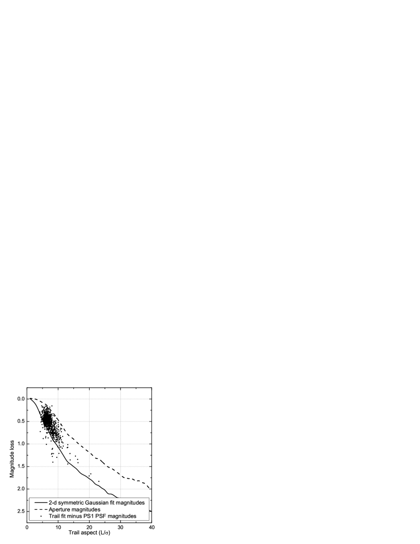
Figure 4: Trailing ‘loss’ as a function of the trail’s aspect ratio (the ratio of its length to width). A perfect algorithm for measuring the magnitude of a trailed detection would provide zero magnitude loss. (solid) The average derived loss in magnitude for synthetic trails fit to 2-d symmetric Gaussians with width equal to the trail width i.e. equal to the PSF. (dashed) The average derived loss in magnitude for synthetic trails using square apertures with sides equal to 3$\times$ the trail width. (data points) The difference in magnitude between the reported Pan-STARRS1 instrumental magnitudes and the correct value for the 1,000 longest real trails for known asteroids.

The trailing loss problem is illustrated in Fig. 4 which shows how the error in the measured or reported magnitude drops as a function of the trail aspect (the ratio of the trail’s length to its width). The figure clearly shows that the trailing loss can induce errors in the flux measurement that are much larger than the statistical uncertainty even for ‘stubby’ trails - those that are trailed only a few times more than their widths. A 2-d symmetric Gaussian fit to the trail is clearly bad. In theory, an aperture magnitude should work very well as long as the aperture is rectangular with its long axis aligned with the trail, of sufficient length to cover the entire trail, and with a width several times the PSF width. The catch-22 is that defining the aperture correctly implies knowing the correct dimension and orientation of the trail in the first place. The aperture magnitudes in Fig. 4 made a simple assumption that the aperture has a dimension equal to 3$\times$ the PSF width so it yields good results to trail aspects of $\sim$3 but degrades quickly thereafter. Assuming larger apertures increases the likelihood of including background flux and thereby increasing the error on the derived flux. The real world Pan-STARRS1 telescope’s Image Processing Pipeline yields excellent photometry on point sources (Schlafly et al., 2012) but fails on trailed sources because it does not implement a trailing fit. Presumably all the contemporary asteroid surveys suffer from this trailing loss at some level.

Due to the worldwide interest in the NEOs, and their relatively high rate of motion that makes them difficult to recover if too long a time passes, NEO candidates are submitted as soon as possible on a per night basis as a set of $\geq 2$ detections known as a ‘tracklet’ (Kubica et al., 2007). Subsequent inter-night linking of tracklets of the same object leads to derivation of the orbit and establishes whether the candidate is in fact a NEO.

Tracklets are constructed by identifying a set of detections that are consistent with being the same object that have moved between exposures. The false tracklet rate is sensitive to the number of detections in the tracklet, the false detection rate, the maximum allowed rate of motion and acceleration, the astrometric and photometric error on each detection, the availability of the detections’ morphological parameters, etc. In practice, the false tracklet rate is surprisingly high, usually due to systematic (rather than statistical) false detections. To reduce the false tracklet rate the Pan-STARRS1 Moving Object Processing System (MOPS; Denneau et al., 2007) implements an upper limit on an object’s rate of motion of 4 deg/day for tracklets containing $\geq 3$ detections and only 0.6 deg/day for tracklets containing just 2 detections. Pan-STARRS1 and contemporary surveys often rely on human observers to identify and verify trails and Pan-STARRS1 is effectively limited to detecting objects with trails $<50$ pixels due to the difficulty in identifying trails and the false tracklet explosion when attempting to link detections of objects that are moving quickly. Fitting all the detections to a trail fitting function helps in every way to reduce the false tracklet rate.

2 The trailing functions

2.1 PSF-convolution trail function

An object moving with a constant apparent angular rate of motion $\omega$ (arcsec/second) in a CCD image with a detector pixel scale $p$ (arcsec/pixel) in an exposure of time $T$ (seconds) leaves a trail of length $L=\omega T/p$ pixels. When $L$ is on the scale of the PSF width the source detection becomes non-PSF like — trailed. We approximate the trail as the convolution of an axisymmetric Gaussian PSF of width $\sigma$ moving at a constant rate in a direction $x^{\prime}$ that is rotated with respect to the image reference frame $(x,y)$. The flux of the trail at any point in the $(x^{\prime},y^{\prime})$ orthogonal coordinate system is then

$$f_{T}(x^{\prime},y^{\prime})=b(x^{\prime},y^{\prime})+\frac{\Phi}{L}\frac{1}{\sqrt{2\pi\sigma^{2}}}\int_{-L/2}^{+L/2}\exp\left[-\frac{1}{2\sigma^{2}}\left\{(x^{\prime}-l)^{2}+(y^{\prime})^{2}\right\}\right]dl$$ (1)

where $\Phi$ is the total photometric flux in the trail and $b(x^{\prime},y^{\prime})$ is the background flux at the same point. The flux in any pixel $(i,j)$ is strictly the integral of $g(x^{\prime},y^{\prime})$ over the bounds of the pixel but in images that are not under-sampled the function changes slowly enough across the pixel that we can assume the pixel flux is simply the flux at the center of the pixel.

This equation can be rewritten using the error function $\mathrm{erf}(z)=\frac{2}{\sqrt{\pi}}{\int_{0}^{z}e^{-t^{2}}\,dt}$, rotating the trail to the image reference frame through an angle $\theta$ with respect to the $+x$-axis, and translating the trail’s centroid to $(x_{0},y_{0})$ such that

$$\begin{split}x^{\prime}=(x-x_{0})\cos\theta-(y-y_{0})\sin\theta\\ y^{\prime}=(x-x_{0})\sin\theta+(y-y_{0})\cos\theta\end{split}$$ (2)

yielding the trail equation

$$\begin{split}f_{T}(x,y)=b(x,y)+\frac{\Phi}{L}\frac{1}{2\sigma\sqrt{2\pi}}\exp\left[-\frac{((x-x_{0})\sin\theta+(y-y_{0})\cos\theta))^{2}}{2\sigma^{2}}\right]\\ \left(\mathrm{erf}\left[\frac{(x-x_{0})\cos\theta+(y-y_{0})\sin\theta+L/2}{\sigma\sqrt{2}}\right]-\mathrm{erf}\left[\frac{(x-x_{0})\cos\theta+(y-y_{0})\sin\theta-L/2}{\sigma\sqrt{2}}\right]\right).\end{split}$$ (3)

It is well known that an axisymmetric Gaussian profile underestimates the flux in real PSFs and other more elaborate PSF models such as the Lorentz or Moffat functional forms could be used (or even empirical functions based on the realized PSFs within an image (e.g. Trujillo et al., 2001)). Any core PSF function can be convolved with a line to provide a trail function though most will of necessity need to be solved numerically. However, the utility of doing so is questionable given that in real images the PSF shape and flux are typically not constant in time — the object leaving a trail may itself be changing its intrinsic flux; the seeing can change during the exposure as may the optical system’s transmission function due to system flexure; wind buffeting, tracking and guiding can change the apparent path of the object on the CCD or its rate of motion across the pixels; etc.

2.2 2-d Gaussian trail function

Elongated detections have classically been recognized when the major axis 2^nd moment significantly exceeds the 2^nd minor axis moment in a fit to a 2-d Gaussian:

$$f_{G}(x^{\prime},y^{\prime})=b(x,^{\prime}y^{\prime})+\frac{\Phi}{2\pi\sigma_{x}^{\prime}\sigma_{y}^{\prime}}\exp\left[-\left(\frac{x^{\prime 2}}{2\sigma_{x^{\prime}}^{2}}+\frac{y^{\prime 2}}{2\sigma_{y^{\prime}}^{2}}\right)\right]$$ (4)

with widths $(\sigma_{x^{\prime}},\sigma_{y^{\prime}})$. Rotating the function using eq. 2 yields

$$f_{G}(x,y)=b(x,y)+\frac{\Phi}{2\pi\sigma_{x}\sigma_{y}}\exp\left[-\left(\frac{(x-x_{0})^{2}}{2\sigma_{x}^{2}}+\frac{(y-y_{0})^{2}}{2\sigma_{y^{\prime}}^{2}}\right)\right]$$ (5)

Fitting a trail to this functional form provides estimates for the centroid position, second order moments, background, and total flux — but not the trail length.

For the 2-d Gaussian we use the major axis 2^nd moment as a proxy for the trail length:

$$L\approx L_{g}=\sigma^{2}_{x^{\prime}}=\int\int\ 2x^{\prime}\int_{-1/2L}^{1/2L}\frac{\Phi}{L}\frac{1}{2\pi\sigma^{2}}\exp\left[-\frac{1}{2\sigma^{2}}\left\{(x^{\prime}-x_{0})^{2}+y^{{}^{\prime}2}\right\}\right]dx_{0}\;dx^{\prime}\;dy^{\prime}.$$ (6)

Integrating equation (6) and dropping the prime notation we find that:

$$L_{g}=\sqrt{12\;(\sigma_{x}^{2}-\sigma_{y}^{2})}$$ (7)

2.3 Acceleration & phase angle effects

Ignoring the topocentric acceleration ($a$) in the trail fit causes an astrometric error at the mid-time of the exposure, the typical time at which astrometry is reported, of $a\;T^{2}/8$ if all the acceleration is parallel to the direction of motion (along-track). Taking as an upper limit a good astrometric error on reported observations of $0.1\arcsec$ than $a\;T^{2}/8\lesssim 0.1\arcsec$ or $a\lesssim 1\arcsec/\;T^{2}$ to guarantee that the acceleration does not induce significant error in the fit. For point of reference, typical exposure times for contemporary asteroid surveys are on the order of 100 s so that accelerations $\gtrsim 10^{-4}$ arcsec/s² induce significant astrometric error.

The fastest topocentric accelerations are observed for objects that are very close to Earth so we examined the apparent rate of motion and acceleration of known asteroids at the moment of their closest approach within 10 lunar distances between 1900 A.D. and 2200 A.D. (see figs. 1 - 3). Of the 601 close approaches only about 2% have accelerations on the order of the canonical limit of $10^{-4}$ arcsec/s². Objects on heliocentric orbits exhibit these accelerations when they are within about one lunar distance (LD), more typically about 0.5 LDs. We note that these objects are moving so quickly across the image plane that they leave very long trails at typical pixel scales — since there is no advantage to long exposures for these trails (the flux per unit trail length is constant) the solution is simply to use shorter exposures to eliminate the astrometric impact of neglecting the objects’ acceleration.

Another possible issue for the astrometric fit to a trail is the effect of changing brightness of the object during the coarse of a single exposure due to the changing phase angle. Figure 2 shows that the fastest moving objects at closest approach to Earth change their brightness at $\gtrsim$0.1 mmag/s so a 100 s exposure would experience $\gtrsim$0.01 mag change in brightness with a mean of $\sim$0.03 mags. This effect is much smaller than typical photometric uncertainty on even slow moving asteroids and comparable to photometric errors induced by variable seeing conditions and sky catalogs. The small asteroids that are typically observed within 1 LD are also rotating on time scales comparable to typical exposure times and the rotation amplitudes are much larger than the phase angle effects (Hergenrother and Whiteley, 2011). Furthermore, linear changes in the brightness will probably not induce large errors in the fitted centroid — only non-linear changes in the flux that occur at an even smaller level. We conclude that the astrometric impact of changing phase angle is extremely small and, in the worst cases as described above, can be ameliorated simply by using shorter exposure times.

Thus, while this work is strictly applicable only to zero acceleration trails with no change in brightness during the exposure, the vast majority of objects exhibit negligible acceleration and brightness change within the exposure time and our technique can be applied without astrometric impact. The method is applicable as long as $a\;T^{2}/8$ is less than the typical astrometric uncertainty which can almost always be achieved simply by decreasing the exposure time.

3 Trail fitting performance

We measured the performance of the trail fitting functions on synthetic and real trails in Pan-STARRS1 images. The synthetic trails were created to mimic the real Pan-STARRS1 trails but allowed us to control the exact flux, position, length and orientation of the trails to determine how well the fitting procedure reproduce the generated values.

We fit the trails to the functions using the IDL procedure mpfit2dfun that employes the Levenberg-Marquardt least-squares fitting technique to minimize the variance between the trail and the model (Levenberg, 1944; Marquardt, 1963).

We imposed several constraints on the fitting procedure to reduce the computation time and reduce the likelihood of non-sensical results. We set the maximum number of iterations to 50 after determining that all good fits were identified by the algorithm in $<50$ iterations and imposed limits on the ranges of the fit parameters — $\sigma$, $L$, $x_{0}$, $y_{0}$. The trail width $\sigma$ is constrained to be within the range of stellar PSF widths from all Pan-STARRS1 images (1.5 pix $<\sigma<$4.5 pix), $L$ must be smaller than the image dimension, and the centroid position ($x_{0}$, $y_{0}$) must be within 20 pixels of the center of the image. The last constraint was implemented because the image ‘source’ detected by the source detection algorithm was placed at the image center.

The resulting fit returned the best values of the 7 fit parameters, $\bar{x}=(b,\Phi,L,\sigma,\theta,x_{0},y_{0})$, and their associated uncertainties, $\delta\bar{x}=(\delta b,\delta\Phi,\delta L,\delta\sigma,\delta\theta,\delta x_{0},\delta y_{0})$. We then calculated the $\chi^{2}$ of the fit in a ‘trail aperture’:

$$\chi^{2}=\sum_{i,j}^{aperture}\frac{[f_{fit}(i,j;\;\bar{x})-f(i,j)]^{2}}{\delta f_{fit}(i,j;\bar{x},\delta\bar{x})}$$ (8)

where $f(i,j)$ is the actual flux in the pixel $(i,j)$, $f_{fit}(i,j)$ is the value of the fit function at pixel $(i,j)$ and $\delta f_{fit}(i,j)$ is the propagated uncertainty in the fit at the same pixel. The ‘trail aperture’ over which the summation is performed has a rectangular shape with center at the fitted centroid position $(x_{0},y_{0})$, length of $L+6\sigma$, width of $3\sigma$, and the long axis of the rectangular aperture is aligned with the major axis of the fitted trail. The reduced chi-squared is $\chi_{red}^{2}=\chi^{2}/(N-7-1)$ where the denominator is the number of degrees of freedom in the fit when ${\it N}$ is the number of the pixels in the aperture. We remind the reader that $\chi_{red}^{2}\sim 1$ for a good fit while much larger or smaller values indicate a bad fit.

In the following sections we quantify the trail fitting algorithms’ performance as a function of the trails’ statistical significance: $S/N=\frac{S}{\sqrt{S+B}}$. The signal $S$ is the integrated flux $\Phi$ of the source as measured by the fit or as generated for synthetic trails. The background $B$ is the integrated total background flux in the trail aperture including readout noise, dark current, sky, and other sources of flux that are not due to the trailed object.

3.1 Generating synthetic trails

Synthetic trails were created using eq. 3. In most astronomical images the background is dominated by the sky and over a small region near a trail the sky is generally flat after correcting for any flat-field issues. Thus, in the absence of noise the flux at a given pixel is $f_{syn}(i,j)=f(i,j;\bar{x})+B$ where $B$ is a constant background level. In the presence of random statistical noise the signal at the pixel is $f^{\prime}_{syn}(i,j)=f_{syn}(i,j)+\mathrm{ran(1)}\sqrt{f_{syn}(i,j)}$ where $\mathrm{ran}(1)$ is a random number from the normal distribution with centroid 0 and width 1.

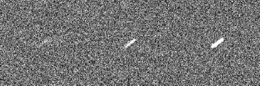
Figure 5: Three synthetic images of synthetic trails with $S/N$= 7, 25, 85. All the trails have $L=30$ pixels, $\sigma$=2 pixels and $\theta=\pi/5=36\deg$.

Figure 5 provides a few examples of synthetic trails where the only difference between them is their $S/N$. The faintest trail at $S/N=7$ is only visible as a faint smudge and the eye is guided to it because we know that the trail lies at the center of that sub-image. Detecting these trails with automated software is not simple — measuring their properties once detected is the purpose of this work.

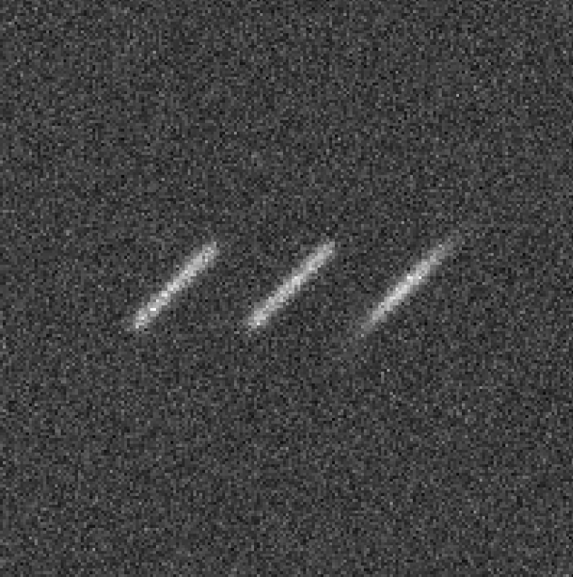
Figure 7: (left) Generated synthetic trail (L=40, $\sigma=2.5$, $\theta=\pi/4$), the same trail reconstructed (center) by the trail fit and the same trail reconstructed with a 2-d Gaussian fit (right).

Figure 6 illustrates the difference between the ‘true’ trail’s profile (eq. 3) and a fit to a 2-d Gaussian (eq. 6). It is clear that in this example the latter can provide reasonable estimates of the trail’s relevant parameters — its flux, centroid and length (perhaps after correction with a simple multiplicative length-based factor). We will show later that the 2-d Gaussian’s utility breaks down for longer trails but its qualitative match to the generated synthetic trails degrades even sooner as shown in figure 7.

3.2 Synthetic trail fitting

We measured the trail fitting performance on 30,000 synthetic trails generated with a flat distribution in length ($10\leq L\leq 50$), orientation ($-90\arcdeg<\theta\leq+90\arcdeg$), width (1.5 pixels $\leq\sigma\leq$ 4.0 pixels), and $3\leq S/N\leq 65$. The range in trail length corresponds to apparent motions of 1.3 to 13.3 deg/day in the Pan-STARRS1 Solar System Survey mode with 45 sec exposure times and a pixel scale of 0.25 arcsec/pixel. The centroids of the synthetic trails were fixed at the center of the small synthetic images.

Figure 8 shows that, as expected, both astrometric error ($\Delta_{x}$) and uncertainty ($\sigma_{x}$) become smaller as $S/N$ increases and $\sigma_{x}\gtrsim\Delta_{x}$. At marginal $S/N$ the error is on the order of 2 pixels. With this metric and for these synthetic trails the 2-d Gaussian fit yields astrometric errors that range from about $\sim 1.5\times$ to $\sim 2.8\times$ higher than the trail fitted errors for $10<S/N<50$. While the astrometric errors are much improved with the trail fitting the reported uncertainties are essentially identical. Thus, the 2-d Gaussian fitting misrepresents the actual error.

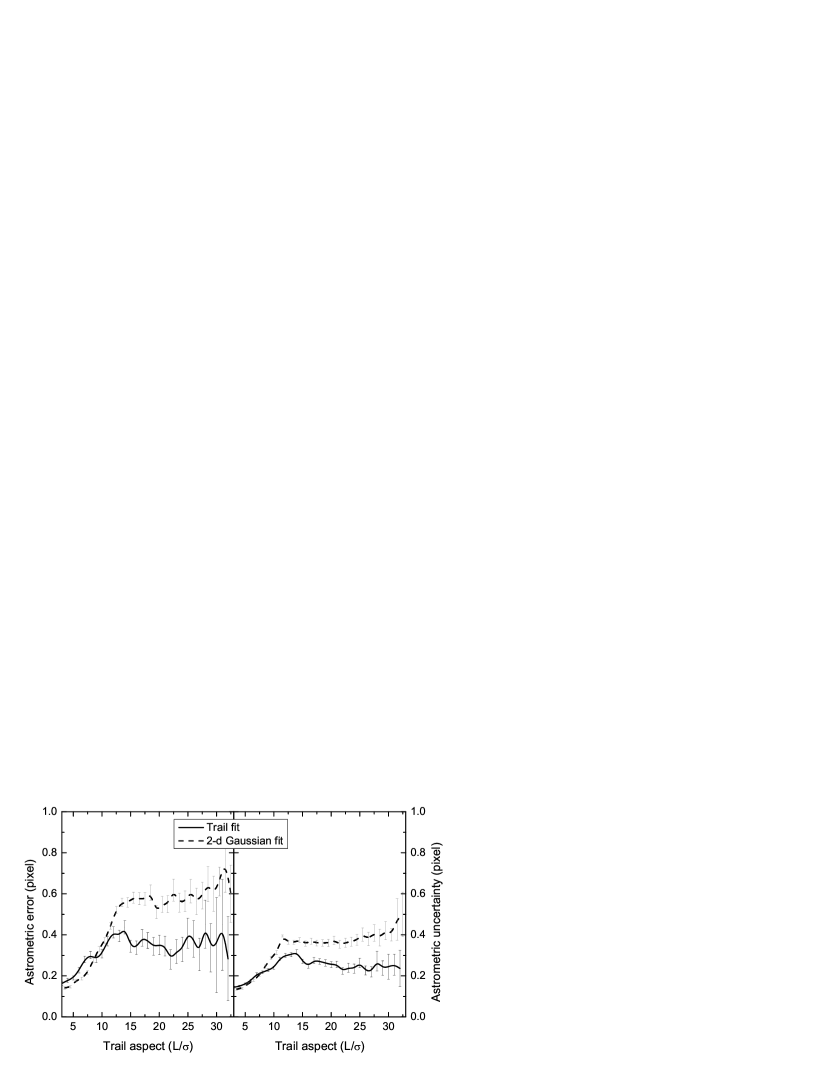
Figure 9: (Left) Moving average of the astrometric error for the PSF-convolution and 2-d Gaussian trail fits as a function of trail aspect ($L/\sigma$) for synthetic trails with $3<S/N<65$. The error bars are the standard error on the mean. (Right) Same as on the left but for the reported uncertainty.

The utility of the trail fitting function is evident in fig. 9 which illustrates how the astrometric error and uncertainty evolve with the trail ‘aspect’: $L/\sigma$, i.e. the length of the trail relative to the PSF. A detection with $L/\sigma\sim 1$ appears untrailed while detections with $L/\sigma\gtrsim 5$ are clearly trailed to eye. The figure shows that as a trail’s aspect increases both the astrometric error and uncertainty increase until they plateau for $L/\sigma\gtrsim 10$. The plateau values are $\sim$50-100% higher for the 2-d Gaussian fit compared to the trail fitting function.

A problem with trailed asteroid detections is the ‘loss’ of $S/N$ as the object becomes trailed. There are two ways to think of this effect: 1) the peak signal per pixel decreases as $1/L$ while the per pixel noise remains roughly constant or 2) the total signal in the trail remains constant as the noise increases because there are more pixels ‘under’ the trail. The former interpretation is a trailing loss because it affects the ability to detect the trail using peak-pixel detection algorithms. The latter interpretation affects the ability of more sophisticated algorithms that attempt to identify trails by integrating the flux along lines. In each case the ability to detect a trailed asteroid decreases due to trailing loss. The amount of trailing loss is not the same in the two classes of algorithms and the implications are too complex to consider in this work that only discusses fitting the trails once they have been identified.

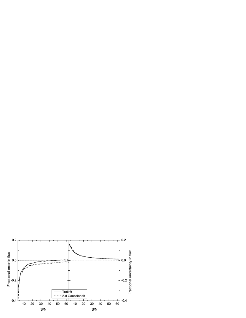
Figure 10: (Left) Fractional error and (right) uncertainty of the flux derived with the trail and 2-d Gaussian fitting as a function of the trail’s total $S/N$. The results include trails of all lengths at the same $S/N$ as described in the text.

Once the trail has been detected it is important to correctly measure the trail’s flux and fig. 10 illustrates the results of the flux determination using the trail and 2-d Gaussian fitting methods. It is clear that the trail fitting is superior to the 2-d Gaussian fit but the figure under-represents the improvements with the trail fitting because it includes trails of all lengths at each total $S/N$. At small total $S/N$ for longer trails the flux is spread over many pixels so that the per pixel $S/N$ is much smaller (the ‘trailing losses’ are described in more detail later in this section). In this situation, by far the most common since the number of trails increases exponentially with decreasing $S/N$, the trail fitting algorithm dramatically outperforms the 2-d Gaussian method.

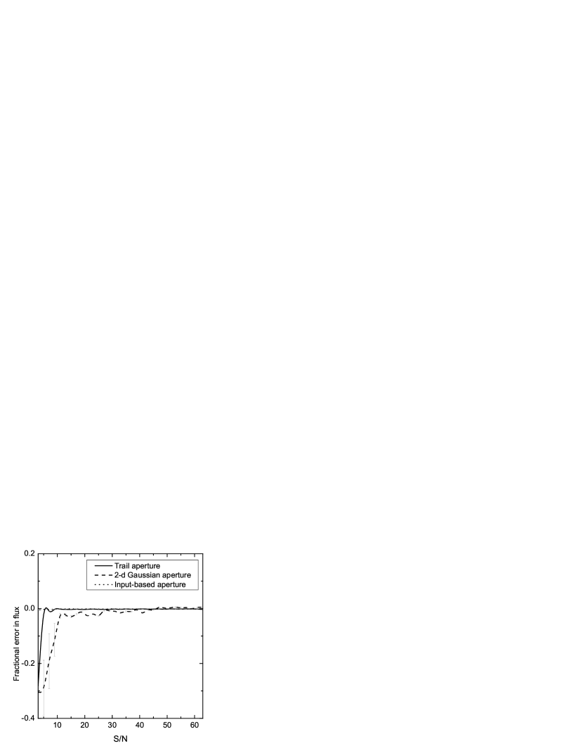
Figure 11: Fractional error of the measured trail flux in rectangular apertures with size and orientation determined by the two types of trail fitting and using the generated (input) parameters versus total $S/N$. The results include trails of all lengths at the same $S/N$.

Figure 11 provides a comparison to the aperture measured photometry using apertures specific to the trail and fit type. i.e. the trail fit uses a rectangular aperture as described in §3 and the 2-d Gaussian aperture uses a similar rectangular apertue but with $L\rightarrow L_{g}$ and $\sigma\rightarrow\sigma_{g}$. We see that trail photometry using apertures based on the generated trail lengths and widths reproduces the expected flux with zero error as expected. An aperture based on the trail-fit length and width performs very well for $S/N\gtrsim 5$ while a flux measurement based on the 2-d Gaussian fit aperture only has approximately zero error for $S/N\gtrsim 25$. Once again, since most trails have small $S/N$-weighted error metric would clearly show that the trail-fitting technique offers a major advantage over the 2-d Gaussian fit.

While the primary purpose of this work was to illustrate the astrometric and photometric improvements when using our PSF-convolution trail fitting the remaining two parameters, the trail length and orientation, are important in linking individual detections on the same night together into ‘tracklets’ (Kubica et al., 2007). This is a common combinatoric explosion when asteroid surveys attempt to link detections of fast moving asteroids — the search area increases as the square of the upper limit on the rate of motion thereby squaring the number of candidate matching detections. One might think that the astrometric and photometric requirements would be sufficient to eliminate false linkages between the detections but, surprisingly, there are often far more false detections than statistics would predict leading to a disturbing number of false tracklets. The typical solution is to decrease the upper rate limit to keep the false tracklet rate manageable and to increase the number of required detections for a valid tracklet.

Another solution to the tracklet formation problem is to use more information — larger areas must be searched as the upper limit on the rate of motion is increased but the faster moving objects will also leave trails rather than point source detections. Those trails will typically be of approximately the same length (assuming constant exposure times) and will have roughly the same orientations. Thus, a good trail fitting algorithm on candidate detections can dramatically reduce the false tracklet formation rate.

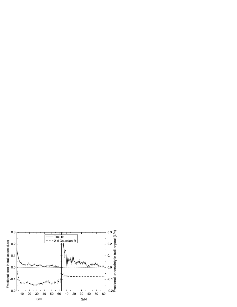
Figure 12: (Left) Moving average of the fractional error on the trail aspect ($L/\sigma$) for the PSF-convolution and 2-d Gaussian trail fits as a function of $S/N$. The error bars are the standard error on the mean. The trail aspect for these synthetic trails ranges from $3<L/\sigma<35$. (Right) Same as on the left but for the reported uncertainty.

The ability to correctly measure the length of a trail is illustrated in fig. 12 in terms of the derived trail aspect error and uncertainty as a function of $S/N$. The length derived with the 2-d Gaussian is always underestimated by $\gtrsim 10\%$ for $S/N\gtrsim 5$ while the PSF-convolution trail fitting provides an error of $\lesssim 3$% in the same $S/N$ range. This is not unsurprising as, by its very nature, the 2-d Gaussian should always underestimate the trail length. The trail aspect uncertainty returned by the 2-d Guassian is always underestimated by about 10% while the trail fit uncertainty is always slightly higher than the error as desired.

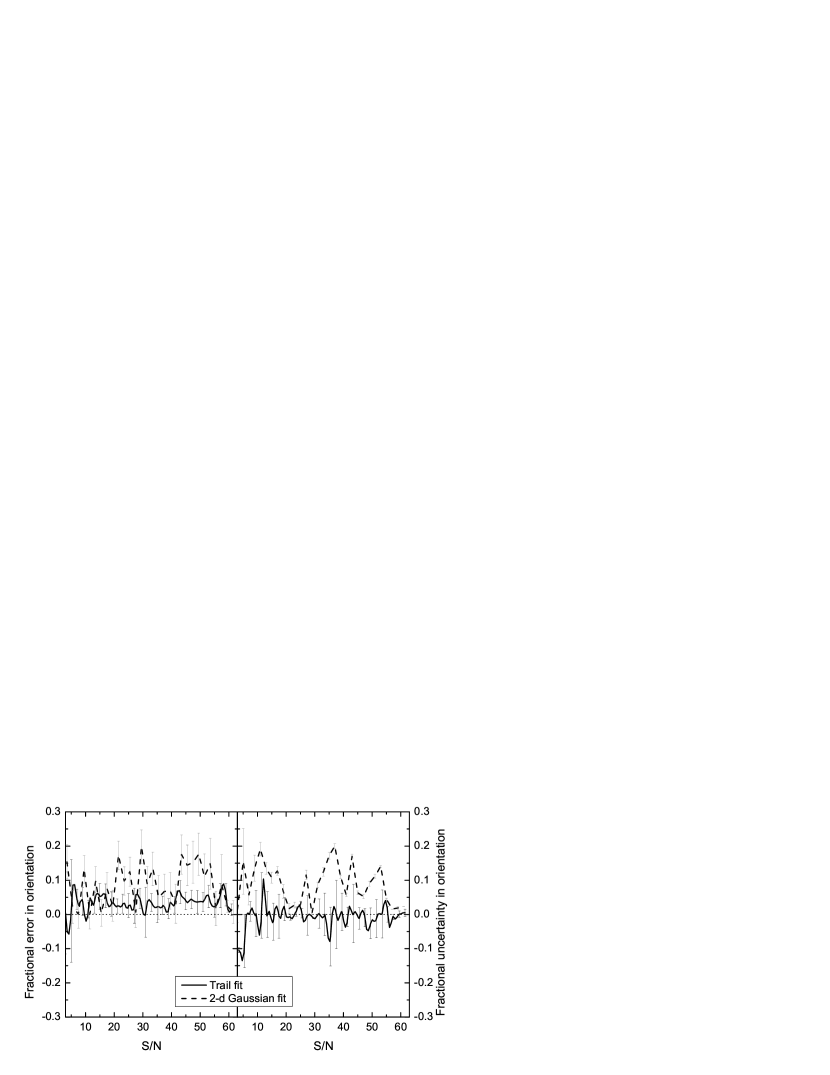
Figure 13: (Left) Moving average of the fractional error on the trail orientation for the PSF-convolution and 2-d Gaussian trail fits as a function of $S/N$. The error bars are the standard error on the mean. The trail aspect for these synthetic trails ranges from $3<L/\sigma<35$. (Right) Same as on the left but for the reported uncertainty.

Similarly, fig. 13 demonstrates that the error in orientation does not depend on the $S/N$ but that the PSF-convolution method consistently performs better than the 2-d Guassian fits. Since the measured trail lengths/aspects and orientations can be used to reduce the false tracklet rate it is important to use a functional form that returns more accurate values and the PSF-convolution trail fit is clearly superior.

4 Real trail fitting

We have shown above that our PSF-convolution trail function performs well on fitting synthetic trails but the true litmus test is how it performs on real detections in real images with all their systematic noise problems, dead and bright pixels, edges and gaps, saturated stars and diffraction spikes, ghost images, cosmic rays, etc.

To test our algorithm on real trails we employed asteroids detected by the Pan-STARRS1 telescope and identified by MOPS. The MOPS database contains hundreds of thousands of known and unknown asteroids of which several thousand are trailed. MOPS stores 200$\times$200 pixel ‘postage stamps’ of all Pan-STARRS1 detections that were incorporated into tracklets. The postage stamp FITS file is the difference of two images of the same portion of the sky exposed at different times (Lupton, 2007) and is therefore already background subtracted.

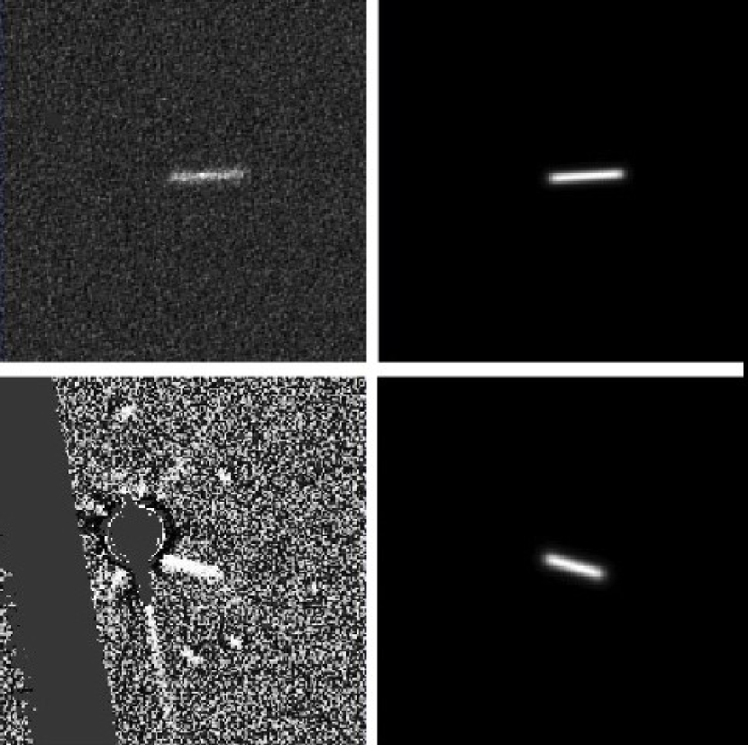
Figure 14: (left) Real Pan-STARRS1 difference images of trailed asteroids and (right) their reconstructed trails from our PSF-convolution trail fitting. (top) An almost ideal case with a nicely trailed detection in the center and no obvious image artifacts and (bottom) a more typical case where the trailed detection passes through the masked pixels of a badly subtracted bright star with diffraction spikes, ‘streaks’, and a gap between CCD chips. Masked or non-existent pixels are in grey.

Figure 14 provides examples of a couple real postage stamps — one ideal and one typical. In the ideal example our trail fitting worked perfectly but even for the more typical case the PSF-convolution trail fit provides a good reconstruction of the visible part of the detection. Even though the trail has been truncated there is still useful information in its orientation and length to assist in linkning similar detections on a night into tracklets. In cases where the trail is truncated our trail fitting algorithm raises a flag that there are masked pixels in the aperture. In these cases the astrometry and photometry are also flagged as suspect.

To measure the astrometric error for real asteroid trails we selected the 1,000 longest trails of numbered asteroid detections from the MOPS database that were submitted to the MPC. These trails have an average length of 15 pixels and the longest automatically detected trail in the sample is 25 pixels long. e.g. an average trail aspect of $\sim$3. For comparison, the average length of the 1,000 longest submitted tracklets irrespective of whether they are known is 18 pixels with the longest being 43 pixels. Since the Pan-STARRS1 survey has not emphasized the detection of trailed, fast moving objects, even longer trails exist in the data that were not detected by the IPP’s source detection algorithms. For instance, we manually identified 114 pixel long trailed detections of 2012 LZ₁ during its close approach to the Earth. These and other trails will be identified and measured as the data are reprocessed but the objects will be impossible to recover. On the other hand, their astrometry and photometry will be useful for future precoveries of the objects by Pan-STARRS1 and other surveys.

We calculated the expected position for each of the 1,000 trailed detections of numbered asteroids at the epoch of observation using OpenOrb (Granvik et al., 2009) that uses DE406 as input for the perturbing planets. Since the numbered asteroids have accurate orbits we can use their calculated positions to measure the astrometric error of our trail fitting method. Figure 15 shows that the PSF-convolution trail fitting provides a 2-3$\times$ improvement in the realized astrometric error over a 2-d Gaussian fit for these trails.

It is clear that figure 15 underestimates the improvement in astrometric error in the trail fitting because we have tested the algorithm only on trails for numbered asteroids. These objects are on average larger, more distant, and leave shorter trails (smaller trail aspects) on the image than the smaller, closer, unnumbered and newly discovered asteroid trails. Reducing the astrometric (and photometric) error on newly discovered objects will have a dramatic impact on the ability to recover the objects shortly after discovery by 1) decreasing the sky-plane ephemeris uncertainty and 2) providing better magnitude estimates to improve target selection by the followup observatories. i.e. to better match the sites’ detection capabilities to the target’s brightness.

As discussed above, false linkages can be dramatically reduced by requiring that the detections within a tracklet have the same orientation (position angle; PA) and roughly the same lengths. The fitted length of real trails is not as robust a filter as the PA because real trails often intersect chip gaps, boundaries, diffraction spikes, etc., that tend to truncate the measured trail length. In practise, the PA filter constraint must be trail length dependent.

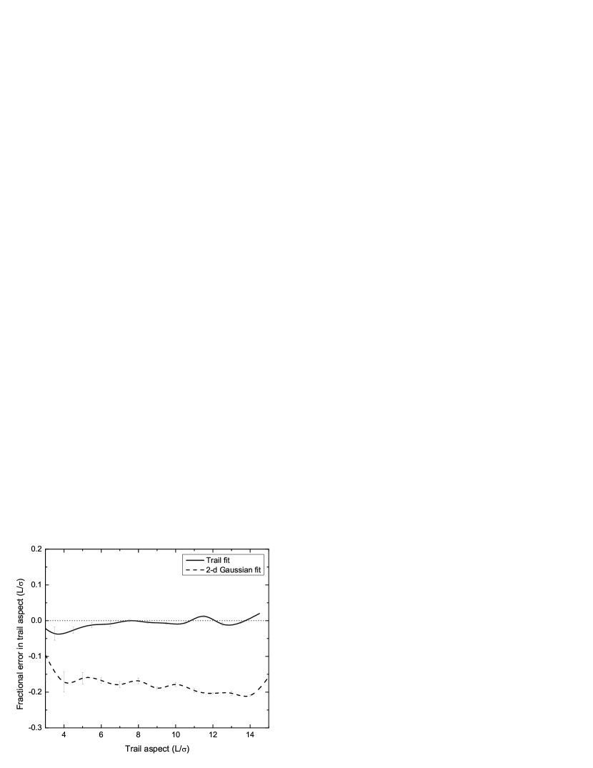
Figure 16: Fractional error in the trail aspect $L/\sigma$ for the 1,000 longest trails for known asteroids for both the (solid) trail fitting and (dashed) 2-d Gaussian fits.

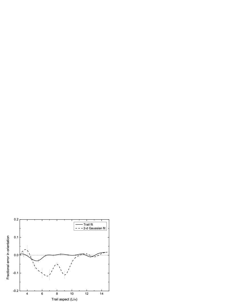
Figure 17: Fractional error in the trail orientation $\theta$ for the 1,000 longest trails for known asteroids for both the (solid) trail fitting and (dashed) 2-d Gaussian fits.

Figures 16 and 17 show the relative error in both measures in our 1,000 trail sample and generally mimic the results from our studies with synthetic trails as shown in figs. 12 and 13. The PSF-convolution trail fit provides lengths (or equivalently, aspects) consistent with the ephemeris prediction but the 2-d Gaussian derived lengths are underestimated by $\lesssim 20$%. The PSF-convolution trail fit derived orientation matches the predicted position angle for all aspect ratios but the 2-d Gaussian-derived orientations show a strange and unexplained error of up to 10% for moderate trail aspect ratios.

One of the major problems with trail identification and characterization is computing time. Even though the human eye and mind are tuned to identify these features writing a computer program to do so in astronomical images and at small $S/N$ has proven to be challenging. Fitting our trail function to a source detection that has already been identified is less time consuming but still $\sim 3\times$ more computationally expensive than simple PSF fitting. For example, Pan-STARRS1 identifies so many false detections that it is computationally impossible with the current hardware resources to fit all identified source detections to the PSF-convolution trail function even though doing so would dramatically reduce the false detection rate.

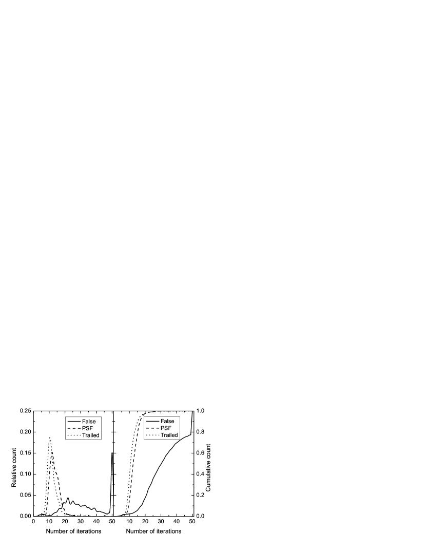
Figure 18: Number of iterations needed for fit convergence for trailed, PSF-like and false detections.

Instead, MOPS currently links detections based purely on the astrometry and consistent motion between detections (Milani et al., 2012) and only fits the PSF-convolution trailing function to those detections vetted and selected by a human observer. Along with the fitted trail’s $\chi^{2}$ we find that we can select for good trails simply by limiting the number of iterations in the fit (see fig.18). The fits to fully 99% of real asteroid detections (both trailed and PSF-like) converged in under 25 iterations while 69% of false detections do not converge. (The number of iterations needed for convergence was tested on a sample of 1,000 trailed, 1,000 PSF-like and 1,000 false detections from Pan-STARRS1.) This is a powerful computational savings since the number of false detections far outnumbers the number of real detections.

4.1 False detection reduction

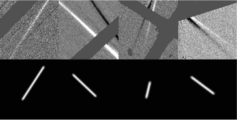
Figure 19: Four examples of (top) diffraction spikes in difference images and (bottom) their corresponding trail fits. The difference images show both the positive and negative diffraction spikes from the same stars but with field rotation between the two images. The trails are only fit to the positive diffraction spikes. The thick gray bands in the difference images represent chip gaps.

Trail fitting is effective at eliminating false detections and even better at eliminating false tracklets. In Pan-STARRS1 images one of the major problems is false detections along diffraction spikes as shown in fig. 19. Statistical fluctuations along the length of the diffraction spikes trigger multiple instances of the PSF-detection algorithm. These false detections can be eliminated by subsequently fitting them to our trailing function because the trail fit returns an unreasonably large RMS and $\chi^{2}$ and position angles that are aligned with the expected PA for diffraction spikes in the image.

We measured the trail fitting’s false detection reduction capability using postage stamps on $\sim$34,000 detections identified by Pan-STARRS1’s PSF-detection algorithm. The maximum number of iterations was set to 25 (as per figure 18) and we required that the fit’s reduced $\chi^{2}<3$. These cuts kept $\sim$96% of real detections and rejected 98% of the false detections.

Tracklet rejection was based on cuts suggested by figures 16 and 17 e.g. detections within a tracklet must have lengths and orientations consistent to within 10% and, as discussed above, the fits can not be compromised by contacting masked detector areas. We achieved a false tracklet rejection rate of 99% while the fraction of rejected real tracklets was only $\sim$1%. The tracklet rejection rate can be higher than the detection rejection rate because the same false detections can appear in multiple tracklets — each of which is rejected by identifying the errant detection.

5 Conclusions

We provide the analytic form for an asteroid trailing function assuming that a symmetrical Gaussian PSF is moving at constant speed during an exposure. We then demonstrate that this function provides accurate photometry and astrometry — much better than the values derived using 2-d Gaussian fits to the trails and much better than the values currently being provided by the Pan-STARRS1 survey.

The trailing function provides astrometry with $>3\times$ smaller errors than are typically reported by the surveys. The photometry with the trail fitting improves by an even larger factor. It is clear that the trail fitting function should be implemented whenever possible — even when fitting stationary objects since they are nothing but trails of length $L=0$. We note that there are extra benefits to using the trailing function for all image sources because the length and orientation can be used to diagnose optical and focus effects within the image plane.

The trail fitting morphological parameters can eliminate on the order of 99% of false tracklets by requiring that detections within the tracklet have the same lengths, orientations, and fluxes. The derived trail lengths and position angles can also help to identify false detections that are saturated streaks and diffraction spikes.

The trail fitting computation time might be an issue because it can be significantly longer than for the 2-d Gaussian. A hybrid method that will be implemented by Pan-STARRS1 is to apply the trail fitting only to detections with large second order moments and/or excessive flux in the aperture that might indicate a trail.

6 Acknowledgements

We would like to thank Jan Kleyna, David Tholen, Marco Micheli, Henry Hsieh, and Eugene Magnier from the Institute for Astronomy at the University of Hawaii for their support and helpful discussions. We thank an anonymous reviewer for helpful feedback. We also thank the PS1 Builders and PS1 operations staff for construction and operation of the PS1 system and access to the data products provided. The Pan-STARRS1 Surveys have been made possible through contributions of the Institute for Astronomy, the University of Hawaii, the Pan-STARRSProject Office, the Max-Planck Society and its participating institutes, the Max Planck Institute for Astronomy, Heidelberg and the Max Planck Institute for Extraterrestrial Physics, Garching, The Johns Hopkins University, Durham University, the University of Edinburgh, Queen’s University Belfast, the Harvard-Smithsonian Center for Astrophysics, and the Las Cumbres Observatory Global Telescope Network, Incorporated, the National Central University of Taiwan, and the National Aeronautics and Space Administration under Grant No. NNX08AR22G issued through the Planetary Science Division of the NASA Science Mission Directorate.

Figure 1: Geocentric distance and apparent rate of motion of known asteroids at the moment of closest Earth approach between the years 1900 and 2200 A.D.

Figure 2: Apparent rate of motion, acceleration, and rate of change in apparent magnitude of known asteroids at the moment of closest Earth approach between the years 1900 and 2200 A.D. (Left) Apparent rate of motion vs. apparent acceleration (Right) Rate of change in apparent magnitude vs. apparent rate of motion.

Figure 3: Along- and cross-trail components of the acceleration of known asteroids at the moment of closest Earth approach between the years 1900 and 2200 A.D. Rates of acceleration above and to the right of the dashed curves are large enough to induce $0.1\arcsec$ astrometric error in the fitted trail position at the specified exposure times of 30, 60 and 100 seconds. i.e. the technique described in this paper does not induce significant astrometric error for rates of acceleration in the lower left corner of the figure.

Figure 6: Profile of a synthetic trail (L = 30, $\sigma=2$, S/N=70) including noise (solid) along its major axis along with the generated trail’s shape (dashed) and the result of a 2-d Gaussian fit (dotted).

Figure 8: (Left) Moving average of the astrometric error for the PSF-convolution and 2-d Gaussian trail fits as a function of the trail’s $S/N$. The error bars are the standard error on the mean. (Right) Same as on the left but for the reported uncertainty.

Figure 15: (solid) Astrometric error after trail fitting for the 1,000 longest trailed detections of numbered asteroids that were submitted to the MPC by Pan-STARRS1and (dashed) for the submitted astrometry from the Pan-STARRS1’s PSF fitting algorithm. For comparison, the average Pan-STARRS1 astrometric error for untrailed detections is $\sim 0.13$ arcsec (Milani et al., 2012).

References

- Denneau et al. (2007) Denneau, L. J., Kubica, J., and Jedicke, R. 2007, in XVI ASP Conference Series, Vol. 376, Astronomical Data Analysis Software and Systems, p. 257
- Granvik et al. (2009) Granvik, M., Virtanen, J., Oszkiewicz, D., and Muinonen, K. 2009, Meteoritics & Planetary Science, 44, 1853
- Hergenrother and Whiteley (2011) Hergenrother, C. W. and Whiteley, R. J. 2011, Icarus, 214, 194
- Jedicke and Herron (1997) Jedicke, R. and Herron, J. 1997, Icarus, 127, 245
- Kaiser et al. (2010) Kaiser, N. et al. 2010, in Proceedings of the SPIE, Vol. 7732, Ground-based and Airborne Telescopes III, ed. G. R. Stepp L.M. and H. H.J., p. 77330E
- Kouprianov (2008) Kouprianov, V. 2008, Advances in Space Research, 41, 1029
- Krugly (2004) Krugly, Y. 2004, Solar System Research, 38, 241
- Kubica et al. (2007) Kubica, J. et al. 2007, Icarus, 189, 151
- Laas-Bourez et al. (2009) Laas-Bourez, M., Blanchet, G., Boër, M., Ducrotté, E., and Klotz, A. 2009, Advances in Space Research, 44, 1270
- Levenberg (1944) Levenberg, K. 1944, Quarterly of Applied Mathematics, 2, 164
- Lupton (2007) Lupton, R. 2007, in ASP Conference Series, Vol. 371, Statistical Challenges in Modern Astronomy IV, ed. B. G.J. and F. E.D., p. 160
- Marquardt (1963) Marquardt, D. 1963, SIAM Journal on Applied Mathematics, 11, 431
- Milani et al. (2012) Milani, A. et al. 2012, Icarus, 220, 114
- Rabinowitz (1991) Rabinowitz, D. 1991, Astronomical Journal, 101, 1518
- Schlafly et al. (2012) Schlafly, E. et al. 2012, eprint arXiv:1201.2208, 1
- Trujillo et al. (2001) Trujillo, I., Aguerri, J., Cepa, J., and Gutiérrez, C. 2001, Monthly Notices of the Royal Astronomical Society, 328, 977