THE INFRARED COLORS OF THE SUN

Abstract

Solar infrared colors provide powerful constraints on the stellar effective temperature scale, but to this purpose they must be measured with both accuracy and precision. We achieve this requirement by using line-depth ratios to derive in a model independent way the infrared colors of the Sun, and use the latter to test the zero-point of the Casagrande et al. (2010) effective temperature scale, confirming its accuracy. Solar colors in the widely used 2MASS $JHK_{s}$ and WISE $W1\,W2\,W3\,W4$ systems are provided: $(V-J)_{\odot}=1.198$, $(V-H)_{\odot}=1.484$, $(V-K_{s})_{\odot}=1.560$, $(J-H)_{\odot}=0.286$, $(J-K_{s})_{\odot}=0.362$, $(H-K_{s})_{\odot}=0.076$, $(V-W1)_{\odot}=1.608$, $(V-W2)_{\odot}=1.563$, $(V-W3)_{\odot}=1.552$, $(V-W4)_{\odot}=1.604$. A cross check of the effective temperatures derived implementing 2MASS or WISE magnitudes in the infrared flux method (IRFM) confirms that the absolute calibration of the two systems agree within the errors, possibly suggesting a 1% offset between the two, thus validating extant near and mid infrared absolute calibrations. While 2MASS magnitudes are usually well suited to derive $T_{\rm{eff}}$, we find that a number of bright, solar-like stars exhibit anomalous WISE colors. In most cases this effect is spurious and traceable to lower quality measurements, although for a couple of objects ($3\pm 2$% of the total sample) it might be real and hints towards the presence of warm/hot debris disks.

1. INTRODUCTION

Photometric systems and filters carry information on various fundamental stellar properties, such as effective temperature ($T_{\rm{eff}}$), metallicity ($\rm{[Fe/H]}$) and surface gravity ($\log g$). Also when studying more complex systems, integrated magnitudes and colors of stars can be used to infer properties of the underlying stellar populations, by interpreting observations via theoretical population synthesis models. However, stars with well known physical parameters and colors are needed to establish how observed photometric data must be translated into physical quantities and placed on an absolute scale. The absolute calibration of photometric systems precisely deal with this matter and it has a long and noble history, especially in using solar-type stars to this purpose (e.g. Johnson, 1965; Wamsteker, 1981; Campins et al., 1985; Rieke et al., 2008). Arguably, the star with best known parameters as well as the most important benchmark in astrophysics is the Sun, but for obvious reasons it can not be observed with the same instruments and under the same conditions applied to distant stars, thus making virtually impossible to directly measure its colors (Stebbins & Kron, 1957).

Photometry of stars with stellar properties very similar to the Sun provides a way to cope with this limit, although it is not obvious how to identify stars satisfying such a condition in first place. Linking photometric measurements to stellar parameters is in fact the goal, and selecting Sun-like stars based on colors would clearly introduce a circular argument. On the other hand, spectroscopy provides an excellent way of determining $T_{\rm{eff}}$, $\log g$ and $\rm{[Fe/H]}$ in stars, and it is routinely used to this purpose, although it can be heavily model-dependent. Nevertheless, this major limit is easily overcome when restricting to a purely differential analysis of stars with spectra largely identical to a reference one. If the latter is solar, it is thus possible to identify the stars most closely resembling the Sun, the so called solar-twins.

Over the last few years, some of us (Meléndez et al., 2006; Meléndez & Ramírez, 2007; Meléndez et al., 2006, 2009; Ramírez et al., 2009) have conducted a systematic search aimed to characterise and discover the best solar-twins in the local $\sim 100$ pc volume, starting from an initial sample of about one hundred stars in the Hipparcos catalogue chosen to be broadly consistent with being solar-like. For each candidate, high resolution, high signal-to-noise observations were conducted and compared to solar reference spectra (which in fact are reflected Sun-light of asteroids) obtained with the same instrumentation and within each observing runs (at McDonald and Las Campanas observatories, see Section 2 in Ramírez et al., 2012).

Because the procedure adopted to identify solar-twins does not assume any a priori $T_{\rm{eff}}$, solar-twins have already been used to set the zero-point of the effective temperature scale via the infrared flux method (IRFM, Casagrande et al., 2010). The effective temperature scale is then a basic ingredient for measuring metallicities and, by comparison with theoretical isochrones, to derive stellar ages. Thus, the zero-point of the effective temperature scale directly impacts basic constraints of Galactic chemical evolution models (e.g the metallicity distribution function and the age-metallicity relation) as well it is important to correctly interpret the Sun in a Galactic context (e.g. Nordström et al., 2004; Casagrande et al., 2011; Datson et al., 2012). Because of its far reaching implications, we have continued to investigate this topic (see also Huber et al., 2012, for a comparison between the angular diameters measured by interferometry with those obtained via the IRFM); in particular we have conducted dedicated observations to overcome the major bottleneck in linking stellar parameters to photometry, i.e. the availability of homogeneous and high accuracy photometric data. In Meléndez et al. (2010) we have presented new Strömgren $uvby$ observations of more than seventy solar-analogs and derived the colors of the Sun in this system, which then have been used to investigate the zero-point of various metallicity scales. Similarly, in Ramírez et al. (2012) we have presented new $UBV(RI)_{\mathrm{C}}\,$photometry of 80 solar-analogs and derived solar colors in the widely used Johnson-Cousins system, obtaining a definitive value for the long debated value of $(B-V)_{\odot}=0.653\pm 0.003$.

In this paper we finally focus on the infrared colors of the Sun and the tight contraints they can provide on the $T_{\rm{eff}}$ scale. In fact, even though it is possible to use Strömgren and Johnson-Cousins colors (Meléndez et al., 2010; Ramírez et al., 2012), infrared ones are better suited to this purpose, being nearly independent on blanketing and surface gravity effects for the spectral types considered here (e.g. Bessell et al., 1998).

In addition to this motivation, highly standardised and precise infrared photometry is nowadays available from all-sky surveys, essentially defining new standard systems for the years to come: 2MASS in the near-infrared, and the WISE satellite in the mid-infrared. Accurate solar colors in these two systems are thus crucial for a numbers of purposes. Most importantly, the reliability at which infrared measurements can be used to infer stellar properties must also be assessed: while 2MASS data can be confidently adopted in most cases, a number of stars seem to exhibit anomalous WISE colors. We find that most of those are artifacts which can be avoided by imposing more stringent observational constraints, although in a few cases they might be real and indicate the presence of debris disks.

2. SAMPLE AND PHOTOMETRIC DATA

Our sample consists of the 112 stars used in Ramírez et al. (2012), from whom we have adopted $V$ magnitudes and stellar parameters. The latter were derived using excitation and ionization equilibrium conditions (Ramírez et al., 2012, and references therein), and because of the strictly differential analysis with respect to the solar reference spectrum, the impact of systematic errors is minimised across the limited parameter space covered by our sample. Although a few stars in our sample might have faint companions, the effect seems negligible for 2MASS, but we detected a few anomalous stars in the WISE colors. As we discuss later, these stars were discarded from the analysis.

For each star we have queried the 2MASS $J\,(1.25\mu\rm{m})$ $H\,(1.65\mu\rm{m})$ $K_{s}\,(2.17\mu\rm{m})\,$ and the WISE $W1\,(3.4\mu\rm{m})\,W2\,(4.6\mu\rm{m})\,W3\,(12\mu\rm{m})\,W4\,(22\mu\rm{m})$ catalogues (Cutri et al., 2003, 2012, respectively) for photometry. Some of the bright targets have saturated or unreliable 2MASS magnitudes; to retain the best data, in a given band we consider only observations having photometric quality flag “A”, read flag “1”, blend flag “1” (i.e. one component fit to the source), contamination and confusion flag “0” (i.e. source unaffected by known artifacts). This set of flags automatically retains stars with photometric uncertainty (“msigcom”) in a given band better than $0.06$ mag, and for the full sample mean errors are $0.02$ mag in $J$ and $K_{s}$ and $0.03$ mag in $H$ band.

Similarly, for WISE observations we restrict our analysis to measurements consistent with being point sources ($\rm{ext}=0$, meaning that no band has a reduced $\chi^{2}>3$ and the source is not within 5 arcsec of a 2MASS Extended Source Catalogue entry), unaffected by known artifacts ($\rm{ccf}=0$), quality flag “A” and variability flag “n” or $0-5$ (i.e. most likely not variable). The “A” quality flag implies a signal-to-noise ratio higher than $10$, automatically curbing large photometric uncertainties. As detailed in the WISE Explanatory Supplement, the $W1-4$ channels saturate at $\sim 8.1,6.7,3.8,-0.4$ mag respectively, although fits to the unsaturated wings of the PSF allow viable magnitudes to be obtained up to $2.0,1.5,-3.0$ and $-4.0$ mag. Given the brightness of our targets, this is never a concern as the saturated pixel fraction is on average $0.07$ in $W1$ and it essentially drops to zero in the other bands. Finally, to further decrease the possibility of having spurious identifications we also require each WISE source to have a 2MASS point source counterpart associated with it. All WISE sources identified with the above constraints have a position offset smaller than 3 arcsec (average $1.5$) with respect to the target coordinate. Some $20-30$ percent of the stars do fall severely apart from the main locus of the color-$T_{\rm{eff}}$ relations, especially in $W2$ and $W4$ band (no such effect is visible using 2MASS), although all quality records listed above are fulfilled (Fig. 1); somewhat arbitrarily we exclude stars having $V-W2\geq 1.65$ and $V-W4\geq 1.80$ and we shall briefly discuss this in Section 4. Altogether, this set of choices limits the mean (max) error to $0.03$ ($0.05$), $0.02$ ($0.02$), $0.02$ ($0.02$), $0.07$ ($0.11$) in $W1,W2,W3,W4$ respectively.

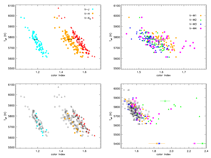
Figure 1.— Color indices versus effective temperatures obtained from the IRFM. Top panels: using only stars satisfying the photometric criteria discussed in Section 2. The colors of the Sun are also shown with the uncertainties derived via the IRFM (Table 3; notice that in the right panel $T_{\rm{eff,\odot}}$ is offset by a few K for clarity purposes). Bottom panels: objects having $V-W2\geq 1.65$ or $V-W4\geq 1.80$ but satisfying all other photometric and quality constraints of Section 2 are highlighted in colors. Stars from the upper panels are now shown with empty circles. In the bottom right panel the effective temperature and color ranges have been increased to include HD 69830 (asterisk); also shown is HD 72905 (pentagram). For both objects WISE’s photometric error bars are shown (see further discussion in Section 4).

3. THE SOLAR INFRARED COLORS

For solar-type stars, $V-J$, $V-H$ and $V-K_{s}$ are known to display a remarkably tight correlation with $T_{\rm{eff}}$, while being nearly independent of other parameters such as $\rm{[Fe/H]}$ and $\log g$. The strong temperature sensitivity in solar-type stars is due to the long wavelength baseline, which almost brackets the region of maximum flux in these stars, covering part of the spectrum with similar continuum opacity but differing temperature sensitivity to the Planck function; this argument continues to hold also when replacing 2MASS with WISE filters (Fig. 1).

In the literature there are various calibrations relating optical/near-infrared indices to effective temperatures of giants and dwarfs (e.g. Ridgway et al., 1980; Alonso et al., 1996; Ramírez & Meléndez, 2005; Casagrande et al., 2010; Boyajian et al., 2012a); for the set of filters used in this work, it can be easily estimated that a change of about $0.03$ mag in solar colors implies an uncertainty of about $50$ K on the zero point of the $T_{\rm{eff}}$ scale. Therefore, to check the reliability of various $T_{\rm{eff}}$ scales, accurate and precise colors must be derived. This is done model independently in Section 3.1, while in Section 3.2 we check upon the zero-point of our effective temperature scale.

For this reason, it is important that the colors under investigation are obtained directly, without resorting on transformations between different systems. Cousins (1987a, b) provides relations between the Strömgren and Johnson-Cousins photometry, and more recently, Bilir et al. (2008, 2011) have derived an extensive set of color transformations relating the 2MASS, WISE and $BV(RI)_{\mathrm{C}}$ systems. Using those, the solar colors derived in Meléndez et al. (2010); Ramírez et al. (2012) and here are usually reproduced within $0.05$ mag (with better performances when transforming from the Strömgren system), although certain color combinations are offset by as much $0.10$ mag, nevertheless still consistent with the standard deviation of the transformations reported in Bilir et al. (2008, 2011).

3.1. Spectral Line-Depth Ratios

Here we use the line-depth ratios (LDRs) technique as described in Ramírez et al. (2012) to derive the infrared colors of the Sun in a model independent way. Briefly, this technique exploits the fact that the ratios of depths of spectral line pairs with very different excitation potential are excellent $T_{\rm{eff}}$ indicators –thus correlating well with observed colors– essentially independent of $\rm{[Fe/H]}$ and $\log g$ (e.g. Gray, 1994). For main sequence stars having $v\,\sin\,i\lesssim 5\,\rm{km\,s}^{-1}$, as the case of our stars, LDRs are also weakly depended on rotational broadening (Biazzo et al., 2007). For each set of line pairs (from Kovtyukh et al., 2003) we measured the ratios in all stars of our sample and linearly fitted those ratios as function of the color index under consideration (Fig. 2), after the exclusion of stars not satisfying the photometric quality requirements discussed in Section 2. From each fit the standard deviation of the fit minus data residual ($\sigma_{\rm{fit}}$) was also obtained. Notice that only line pairs for which the color vs. LDR slope was greater than $0.3$ have been used. Slopes shallower than this imply a lower sensitivity, leading to larger errors in the derived solar color. Since the slope errors are about $0.03$, this criterion is equivalent to a $10\,\sigma$ cut. An example of all line pairs used to derive the solar $(V-K_{s})$ color is given in Table A. The interpolation of those fits at the solar ratio (measured in the reflected Sun-light of asteroids with the same procedure used for stars) returns the color index of the Sun. Since we have nine reflected Sun-light observations, nine solar line-depth ratio values are available for each line pair, resulting in nine solar colors. Columns 7 and 8 of Table A provide the mean and standard deviation ($\sigma_{\rm{ss}}^{2}$) of those nine values. For each color index there are usually about one hundred pairs available, thus making possible to derive extremely robust colors (Table 2), using the weighted mean of the values obtained from each line-depth ratio, where the weight $w$ is $1/w=\sigma_{\rm{fit}}^{2}+\sigma_{\rm{ss}}^{2}$ (see also Ramírez et al., 2012).

Figure 2.— Observed colors as a function of line-depth ratio for the 6119.53 Å (V I), 6145.02 Å (Si I) pair. The solid line is a linear fit to the data.

Table 2Solar colors inferred from LDR Measurements.

color	value	$N_{\mathrm{pairs}}$
$(V-J)$	$1.198\pm 0.005$	87
$(V-H)$	$1.484\pm 0.009$	102
$(V-K_{s})$	$1.560\pm 0.008$	100
$(V-W1)$	$1.608\pm 0.008$	101
$(V-W2)$	$1.563\pm 0.008$	102
$(V-W3)$	$1.552\pm 0.009$	103
$(V-W4)$	$1.604\pm 0.011$	92

3.2. Color-$T_{\rm{eff}}$ Relations

Table 3Solar colors inferred from different $T_{\rm{eff}}$ measurements: spectroscopic (i.e. excitation and ionization equilibrium) and the IRFM implemented using Tycho2$+$2MASS (TY2M) or Johnson-Cousins$+$2MASS (JC2M) photometry.

color	spectroscopic	$\rm{IRFM_{TY2M}}$	$\rm{IRFM_{JC2M}}$	$N_{\mathrm{stars}}$
$(V-J)$	$1.207\pm 0.013$	$1.197\pm 0.013$	$1.185\pm 0.013$	87
$(V-H)$	$1.499\pm 0.014$	$1.489\pm 0.013$	$1.475\pm 0.014$	87
$(V-K_{s})$	$1.572\pm 0.013$	$1.563\pm 0.013$	$1.549\pm 0.013$	95
$(V-W1)$	$1.620\pm 0.015$	$1.613\pm 0.014$	$1.601\pm 0.016$	52
$(V-W2)$	$1.576\pm 0.011$	$1.570\pm 0.011$	$1.561\pm 0.012$	56
$(V-W3)$	$1.564\pm 0.013$	$1.558\pm 0.014$	$1.545\pm 0.016$	59
$(V-W4)$	$1.610\pm 0.021$	$1.601\pm 0.018$	$1.592\pm 0.018$	42

The technique presented in Section 3.1 provides an elegant and model independent way of determining the colors of the Sun. Alternatively, it is possible to perform a multiple regression of the stellar parameters (e.g. $T_{\rm{eff}},\log g,\rm{[Fe/H]}$) relevant to a given color index and derive that of the Sun by solving with respect to its parameters (e.g. Holmberg et al., 2006; Meléndez et al., 2010; Ramírez et al., 2012). Works focusing on the $T_{\rm{eff}}$ scale adopt essentially the same approach, where the colors of the Sun are inferred by reverting polynomial $\rm{color}-\rm{[Fe/H]}-T_{\rm{eff}}$ relations derived for dwarf stars (e.g. Ramírez & Meléndez, 2005; Casagrande et al., 2006). While indices in Table 2 tightly correlate with $T_{\rm{eff}}$, because of the relatively narrow parameter space covered by of our stars, we have verified that they do not display any significant dependence on $\log g$ nor $\rm{[Fe/H]}$. In fact, performing a multiple linear regression with respect to all three parameters or $T_{\rm{eff}}$ only did not improve upon the residual nor changed within $0.001$ mag the values derived. Such a simple linear relation has also the advantage of making straightforward the connection between a given color index and the underlying $T_{\rm{eff}}$ scale. Depending on the band considered, several tens of stars survive the quality cuts we impose on 2MASS/WISE photometry (Section 2 and Table 3). Using the spectroscopic (excitation and ionization equilibrium) temperatures determined for the full sample of solar-analogs returns solar indices systematically redder by $\sim 0.01$ mag with respect to those obtained via LDRs. This implies that on average our spectroscopic $T_{\rm{eff}}$ are overestimated by about $20$ K, in agreement with what found by Ramírez et al. (2012) using optical indices.

For all stars in our sample we also run the IRFM to derive effective temperatures uncorrelated to the spectroscopic analysis. In fact, the IRFM is essentially model independent and very little affected by the metallicity and surface gravity of each star, the most relevant ingredient being the absolute calibration of the photometric systems adopted. Since all these stars are nearby, reddening is also not a concern as confirmed by using intrinsic Strömgren color calibrations (Meléndez et al., 2010). In Casagrande et al. (2010) the zero point of the IRFM scale was calibrated using solar-twins having Tycho2 and 2MASS photometry. Now, the availability of $UBV(RI)_{\mathrm{C}}\,$magnitudes allows to check whether this is also the case when using instead the Johnson-Cousins system. Replacing the Tycho2 with the Johnson-Cousins system in the IRFM returns effective temperatures cooler by $26\pm 4$ K ($\sigma=41$ K) which is within the zero-point uncertainty of our effective temperature scale. The same conclusion is obtained restricting the analysis to solar-twins only for which we obtain a median/mean $T_{\rm{eff}}$ of $5787/5786$ K and $5762/5750$ K using Tycho2 and Johnson-Cousins photometry, respectively. These differences are mirrored in the color indices of Table 3: those inferred using Johnson-Cousins in the IRFM are in fact slightly bluer than obtained via LDRs, by an amount which would be almost perfectly offset should the effective temperatures increase by $20$ K. As expected, $(V-J)_{\odot}$, $(V-H)_{\odot}$ and $(V-K_{s})_{\odot}$ derived here agree extremely well with those obtained by Casagrande et al. (2010) reverting $\rm{color}-\rm{[Fe/H]}-T_{\rm{eff}}$ polynomials defined over a much wider parameter space.

Effective temperatures determined using Tycho2 photometry in the IRFM return color indices which agree almost perfectly with LDRs. These results confirm the overall good consistency obtained implementing different photometric systems in the IRFM, with systematic uncertainties at the level of about $20$ K, i.e. $\sim 0.01$ mag in colors. Errors in Table 3 take this into account, by adding such zero-point systematic to the uncertainties derived analytically from the fits.

4. The WISE through excess of infrared is made a fool?

As discussed in Section 2, stars having exceedingly red indices in WISE (Table 4) were not used to derive solar colors, although all other photometric quality constraints were satisfied (apart from a few cases having in a given band $\rm{ccf}\neq 0$ or signal-to-noise lower than 10, bands which were always excluded from the analysis). The unusual colors of these stars are clearly visible in the bottom right panel of Figure 1. The bands most strikingly affected are $W2$ and partly $W4$, while $W1$ and $W3$ seem only slightly offset to the red with respect to the main locus defined by the full sample. This sort of signature ($W1-W2\gtrsim 0.3$) would not be entirely unexpected if looking at brown dwarfs. In fact, WISE’s two shortest bands are designed to optimize sensitivity to this class of objects, by probing their deep $\rm{CH}_{4}$ absorption band at $\sim 3.3\mu\rm{m}$ ($W1$) and the region relatively free of opacity at $\sim 4.6\mu\rm{m}$ ($W2$) where their Planck function approximately peaks (e.g. Wright et al., 2010; Mainzer et al., 2011; Kirkpatrick et al., 2011).

To quantify the amount of contamination expected from a potential low mass star companion we combine a synthetic MARCS (Gustafsson et al., 2008) solar spectrum with that of a late type M dwarf ($T_{\rm{eff}}=2500$ K) of the same metallicity, and assuming a secondary to primary radius ratio of $0.2$ (Boyajian et al., 2012b), we conclude that the effect on the color indices shown in Figure 1 would be of order $0.01$ mag. Therefore, even if the spectral features of a brown dwarf could account for the red $W1-W2$ index we observe, the overwhelming flux of the primary makes this solution not viable even for an M dwarf, in addition to the fact that it would still be difficult not to affect $W3$ . Neither the alignment/confusion with extragalactic sources (which would be considerably fainter than our objects, see below) or cool (sub)-stellar objects is likely. The angular resolution of WISE passes from $6.1$ arcsec in $W1$ to $12$ arcsec in $W4$; using the higher resolution of 2MASS, none of the targets discussed here has more than one counterpart within $12$ arcsec. All anomalous sources have $W1$ brighter than $7.6$ mag ($5.9$ mag if considering the reddest $V-W2>1.8$). Using this constraint with the previous synthetic model ($T_{\rm{eff}}=2500$ K) would imply the presence of cool M dwarfs closer than $7.5$ ($3.5$) pc and brighter than $V\sim 17$ ($15.5$) mag. Using instead a synthetic brown dwarf spectrum ($T_{\rm{eff}}=1000$ K, Burrows et al., 2006) and adopting $R=0.1R_{\odot}$ the above estimates would change into distances closer than $1$ ($0.5$) pc and $V$ magnitudes brighter than $\sim 21$ ($19.5$) mag, thus making extremely unlikely the superposition of brown dwarfs to our solar-like stars.

Interpreting the color anomaly as mid-infrared emission could hint toward the presence of warm/hot debris disks, even though this class of object is thought to be very rare compared to most of the known cold Kuiper-belt type disks, especially around old main sequence stars (e.g. Bryden et al., 2006; Wyatt, 2008). In Figure 1 it is interesting to include for comparison HD 69830 (HIP 40693), a $\sim 2-4$ Gyr old, solar metallicity dwarf known to host a warm disk closer than $\sim 1$ AU (Beichman et al., 2005) as well as three Neptune-mass planets within $0.6$ AU (Lovis et al., 2006). Although HD 69830 has a $T_{\rm{eff}}$ somewhat cooler than the bulk of our stars (Sousa et al., 2008), it shows a clear excess in $W2$ and $W4$, while $W1$ and $W3$ are barely affected. A somewhat similar trend is also shown by HD 72905 (HIP 42438), a $\sim 0.2$ Gyr old, solar-like star surrounded by hot dust (Beichman et al., 2006).

However, producing emission in $W2$ while keeping the other two contiguous bands essentially unaffected requires major fine tunings, thus rendering also the disk interpretation difficult. At first, interpreting all anomalous WISE colors as suspected and/or poor photometry seems difficult because of the various quality constraints imposed (Section 2), although a number of W2 excesses have a saturated pixel fraction higher than usual (c.f. Section 2) and more stringent cuts do alleviate the problem. Kennedy & Wyatt (2012) have conducted a throughout study of stars in the Kepler field using WISE photometry to identify disk candidates, and concluded in fact that spurious detections are less likely when using photometric measurements with source extraction $\chi^{2}$ smaller than $2,\,1.5,\,1.2,\,1.2$ in $W1-4$, respectively. The requirement $\rm{ext}=0$ we adopt is in fact less stringent (Section 2); the tighter $\chi^{2}$ constraints listed above are satisfied by $98\%$ ($W1$), $80\%$ ($W2$), $53\%$ ($W3$), $93\%$ ($W4$), of the stars used in Section 3, and by $100\%$ ($W1$), $50\%$ ($W2$), $50\%$ ($W3$), $95\%$ ($W4$) of the stars in Table 4. This suggests that any excess we see in $W4$ might be real, but it casts some doubts on $W2$. Adopting these constraints the number of outliers in Table 4 considerably reduces, although a number of them still remains: HIP 109110, objects with excess in $W2$ only (HIP 38228, HIP 88194 HIP 100963) and $W4$ only (HIP 38072 and HIP 66885).

For these six stars (plus HD 69830 and HD 72905), photospheric models tailored at the measured spectroscopic parameters are compared to fluxes derived from the adopted photometry (Figure 3). The absolute calibration of those model fluxes is done by forcing them to return synthetic $V$ magnitudes that match the observed ones. We also tested on the full sample of stars in Section 2 that the mean difference in physical fluxes is $0.25\%$ and never exceeds $1.5\%$ if doing instead the absolute calibration using angular diameters obtained from the IRFM. These differences are essentially indistinguishable on the scale of the plot, and are taken into account when computing the flux uncertainty associated to each photometric measurement. Magnitudes in the $BV(RI)_{\mathrm{C}}\,JHK_{s}$ system are converted into fluxes using the same absolute calibration adopted in Casagrande et al. (2010), which has an intrinsic uncertainty of order $1-2\%$. Because of the aforementioned difference between using $V$ magnitudes or angular diameters, we have increased the global flux error to a conservative $3\%$. Similarly, for the $WISE$ system, we have adopted the absolute calibration and errors from Jarrett et al. (2011), further increasing the latter by $1\%$, which also takes into account the possible zero-point offset discussed in Appendix A. Observed magnitude errors are then added to the aforementioned uncertainties regarding the absolute flux of each band. As already expected from color indices, any difference with respect to photospheric models in $W2$ and $W4$ is significant, and it does not stem from uncertainties on the flux scale, nor in the observed magnitudes. The advantage of fitting photospheric models instead of using color indices is that we are now able to better quantify the observed anomalies. The same comparison with synthetic spectra have also been done for all other stars in our sample not showing anomalous WISE colors, and indeed there are no mismatches between synthetic spectra and observations, thus validating the overall flux scale we adopt and also excluding major model deficiencies in those bands for solar-like stars (but see Kennedy & Wyatt, 2012, for possible model inaccuracies at cooler $T_{\rm{eff}}$).

As we already discussed, adding a cool companion does not modify the energy distribution in a way which is able to explain the observations, apart from HIP 109110, which longward of the $J$ band shows fluxes systematically higher than predicted. This likely indicates the presence of a cool companion (which we are able to fit with a model having $T_{\rm{eff}}\sim 4000$ K), an interpretation which is consistent with its suspected binarity (Frankowski et al., 2007) and with the linear trend observed in its radial velocity (Nidever et al., 2002). This infrared excess is then further confirm by the Spitzer-IRAC and -MIPS measurements (Carpenter et al., 2008) shown in Figure 3 as open squares.

The $W2$ measurements for HD 69830 and HD 72905 do not pass the more stringent requirements we impose on the source extraction. The spurious nature of $W2$ photometry for these two stars is then confirmed by the absence of excess in other measurements at similar wavelengths (Carpenter et al., 2008; Beichman et al., 2011). Note though, for HD 69830 the IRS, Spitzer-MIPS and IRAS data (Beichman et al., 2011) confirm the excess we see in $W4$. Thus, we are inclined to regard any $W2$ excess among our stars as artificial, even if the source extraction is fine; this is further supported by the fact that in Figure 3 the $W2$ photometry of HIP 100963 does not agree with Spitzer-IRAC (Carpenter et al., 2008). No additional measurements around $4.6\mu\rm{m}$ exist for HIP 38228 and HIP 88194, but from the previous discussion, and because these excesses seem rather challenging to interpret when contiguos bands agree well with photospheric models, we conclude that also their nature is likely spurious.

Finally, for HIP 38072 and HIP 66885 the deviation from photospheric models starts only in $W4$. Despite these two stars being the faintest among those in Table 4, so far our adopted quality constraints have been enough to discard unreliable $W4$ measurements, and what we see could be indeed the signature of debris disks around these two stars. For HIP 38072 we have a measured flux of $10.7\pm 0.7$ mJy and a photospheric prediction of $6.7\pm 0.2$ mJy, thus resulting in an excess ratio of $1.6$ with a $5\sigma$ significance, while for HIP 66885 the measured flux is $8.7\pm 0.8$ mJy versus a photospheric prediction of $7.0\pm 0.2$ mJy, the excess ratio being $1.2$ at $2\sigma$. Using the absence of emission in $W3$ to constrain their temperature, we are able to easily fit these excesses with a black-body, but measurements at other wavelengths are clearly required to confirm or discard the presence of any disk. Should these two detections be confirmed, and using the variance of the the binomial distribution to derive a realistic error bar for such a low number statistic (e.g. Bevington, 1969) the occurrence rate of debris disk at $22\mu\rm{m}$ from our solar-like sample would thus be $3\pm 2$%, in good agreement with the $\sim 4$% estimated by Trilling et al. (2008) at $24\mu\rm{m}$.

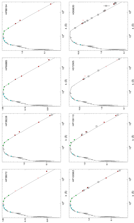
Figure 3.— Observed fluxes vs. photospheric models (from Castelli & Kurucz, 2004) for stars still having anomalous WISE colors after imposing more stringent requirements on the source extraction. Fluxes $-\,F_{\nu}\rm{(Jy)}\,-$ are derived from optical (cyan), 2MASS (green) and WISE (red) magnitudes as described in text: filled (open) symbols identify WISE photometric measurements that do (not) satisfy the requirements discussed in Section 4, including the stricter $\chi^{2}$ extraction threshold. Open squares are independent flux measurements available in literature (Carpenter et al., 2008; Plavchan et al., 2009; Beichman et al., 2011).

Table 4Stars having $V-W2\geq 1.65$ or $V-W4\geq 1.80$. Bands that do not satisfy all of the quality constraints discussed in Section 2 are written in italics. The $\chi^{2}$ of the source extraction in each band is given in parenthesis.

HIP	$V$	$W1$	$W2$	$W3$	$W4$
8507	$8.899$	$7.185$	$7.217$	$7.230$	$7.109$
		$(1.45)$	$(1.25)$	$(1.00)$	$(1.09)$
11072	$5.190$	${\it 3.607}$	$2.903$	$3.631$	$3.594$
		$(0.28)$	$(2.09)$	$(2.12)$	$(1.04)$
12186	$5.785$	$4.241$	$3.741$	$4.252$	$4.210$
		$(0.73)$	$(2.25)$	$(1.71)$	$(0.87)$
15457	$4.836$	${\it 3.334}$	${\it 2.614}$	$3.334$	$3.243$
		$(0.38)$	$(1.21)$	$(1.66)$	$(0.96)$
22263	$5.497$	$3.956$	$3.467$	$3.981$	$3.912$
		$(0.37)$	$(2.04)$	$(1.37)$	$(0.93)$
29525	$6.442$	$4.768$	$4.475$	$4.857$	$4.800$
		$(0.33)$	$(1.70)$	$(0.76)$	$(0.91)$
38072	$9.222$	${\it 7.627}$	${\it 7.678}$	${\it 7.626}$	$7.227$
		$(1.57)$	$(0.90)$	$(1.26)$	$(1.21)$
38228	$6.900$	$5.198$	$5.048$	$5.293$	$5.170$
		$(0.42)$	$(1.30)$	$(0.79)$	$(1.17)$
44713	$7.306$	${\it 5.650}$	${\it 5.629}$	${\it 5.744}$	$5.717$
		$(0.49)$	$(1.26)$	$(1.14)$	$(0.96)$
55459	$7.646$	$5.965$	$5.990$	$6.045$	$5.994$
		$(0.63)$	$(1.53)$	$(0.92)$	$(0.89)$
57291	$7.466$	$5.802$	$5.730$	$5.831$	$5.694$
		$(1.05)$	$(1.25)$	$(1.35)$	$(1.16)$
66885	$9.302$	$7.638$	$7.691$	$7.665$	$7.445$
		$(1.05)$	$(0.88)$	$(1.13)$	$(0.92)$
77052	$5.868$	$4.129$	$3.547$	$4.166$	$4.143$
		$(0.65)$	$(2.02)$	$(1.73)$	$(0.83)$
80337	$5.391$	$3.919$	${\it 3.378}$	${\it 3.902}$	$3.834$
		$(0.74)$	$(2.03)$	$(0.65)$	$(0.74)$
85042	$6.287$	${\it 4.676}$	${\it 4.240}$	$4.708$	$4.657$
		$(0.89)$	$(2.14)$	$(0.85)$	$(0.82)$
88194	$7.101$	$5.472$	$5.343$	$5.506$	$5.492$
		$(0.94)$	$(1.32)$	$(1.74)$	$(1.15)$
96895	$5.959$	${\it 4.385}$	${\it 4.004}$	${\it 4.444}$	$4.412$
		$(0.47)$	$(1.66)$	$(0.78)$	$(0.92)$
100963	$7.089$	$5.517$	$5.416$	$5.583$	$5.538$
		$(0.52)$	$(1.08)$	$(0.75)$	$(1.06)$
109110	$7.570$	$5.870$	$5.743$	$5.857$	$5.810$
		$(1.22)$	$(1.01)$	$(1.18)$	$(0.92)$
113357	$5.467$	$3.881$	$3.361$	$3.927$	$3.914$
		$(0.29)$	$(1.75)$	$(2.38)$	$(0.84)$

5. CONCLUSIONS

The uncertainty on the zero point of the effective temperature scale has been addressed using one of the most stringent photometric contraints available, i.e. the infrared colors of Sun, here determined in a model independent way via LDRs. Such analysis leads to an excellent agreement with the indices derived using the $T_{\rm{eff}}$ scale of Casagrande et al. (2010), thus confirming its accuracy. Effective temperatures have also been determined implementing the IRFM in the WISE system, thus validating the overall consistency between the 2MASS and WISE absolute calibration. This work also shows the importance of using solar twins for the absolute calibration of photometric quantities, something which is getting increasingly more important in the era of large all-sky photometric surveys.

However, while 2MASS magnitudes are very well suited for the purpose of determining $T_{\rm{eff}}$ –once stars affected by binarity are removed and/or using the full quality and flag information available in 2MASS to discard bad photometry– this does not necessarily hold for the WISE data. Special attention on WISE’s photometric quality flags and source extraction information must be paid, yet a number of excess emissions in $W2$ seem artificial. In this respect 2MASS magnitudes lie in a “sweet spot”, enough in the red to sample the Planck tail, yet largely unaffected by contamination and/or flux excess, that being real or spurious.

At this stage it is still unclear if all WISE mid-infrared anomalies found are stemming from bad measurements or they are rather associate to real physical phenomena. Either cases being possible, those stars are clearly not representative of the Sun and have not been used to derive its colors. It is extremely difficult to interpret in a consistent manner objects showing intense excess in $W2$ only (and in fact, comparison with independent measurements confirms the spurious nature), while on the contrary it seems genuine for $W4$. This latter excess could be the signature of warm/hot debris disks, the best candidates from our sample being HIP 38072 and HIP 66885. Data at longer wavelengths are clearly needed: should HIP 38072 be confirmed, it would be the first solar-analog/twin ($T_{\rm{eff}}^{\rm{{\tiny spec}}}=5839$ K, $\log g=4.53$ dex, $\rm{[Fe/H]}=0.06$ dex) found to host such a debris disk. This star is also relatively young ($2.4$ Gyr) and has $\sim 4$ times more lithium than the Sun (Baumann et al., 2010), and it is included in our HARPS radial velocity monitoring, thus making it a potentially interesting target to gauge new insights into the planet–disk interaction.

Note added in proof. The reason for the anomalously bright $W2$ magnitudes likely stems from problems in the profile fitting photometry for bright saturated stars, see http://wise2.ipac.caltech.edu/docs/release/allsky/expsup/
sec6$\_$3c.html

Appendix A The InfraRed Flux Method using WISE photometry

The availability of 2MASS and WISE photometry for most of the stars in our sample permits to run the IRFM using these two systems separately, and to check that consistent effective temperatures are derived. The implementation of the method is identical to that described in Casagrande et al. (2006, 2010), i.e. for each star the bolometric flux is recovered using all available broad-band optical/near-infrared/mid-infrared colors, while infrared fluxes needed to derive $T_{\rm{eff}}$ are now computed using 2MASS or WISE photometry, respectively.

For solar-type stars, the main driver in setting the zero-point of the $T_{\rm{eff}}$ scale is the absolute calibration of infrared bands. We have already discussed and tested that of 2MASS (Casagrande et al., 2010, and references therein), thus focusing on the WISE system here. We adopt the $W1\,W2\,W3\,W4$ relative system response curves and physical monochromatic fluxes $F_{\lambda}\rm{(iso)}$ from Jarrett et al. (2011). The latter are built on the same absolute basis established for the Spitzer Space Telescope, ultimately constructed on the “Cohen-Walker-Witterborn ” framework (Cohen et al., 2003, and references therein) and tied directly to the absolute mid-infrared calibrations by the Midcourse Space Experiment (MSX, Price et al., 2004). These WISE fluxes have an expected overall systematic uncertainty of order $\sim 1.5\%$ and define the Vega zero-magnitude attributes upon which the effective temperatures we derive in this system directly depend. For each star we used the photometric constraints discussed in Section 2 and derived $T_{\rm{eff}}$ if at least two WISE bands were simultaneously available. $W4$ magnitudes have the largest photometric errors (Section 2) thus showing the weakest correlation with $T_{\rm{eff}}$; indeed the scatter in the comparison with the effective temperatures obtained using 2MASS magnitudes reduces when $W4$ is not implemented in the IRFM (Figure 4).

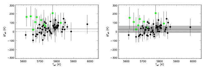
Figure 4.— $\Delta T_{\rm{eff}}(\rm{2MASS}-\rm{WISE})$ when implementing one or another system in the IRFM. Filled squares are stars having $V-W2$ and $V-W4$ redder than the thresholds discussed in Section 2, and are not used to derive the mean difference (continuous line). Left panel: using in the IRFM at least two bands among $W1\,W2\,W3\,W4$. Right panel: when restricting to at least two bands among $W1\,W2\,W3$. Gray shaded area is the systematic offset ($\pm 36$ K) allowed by the uncertainty in the WISE’s absolute calibration.

The maximum zero-point uncertainty in the effective temperatures derived using WISE photometry can be easily estimated by increasing or decreasing the adopted absolute calibration according to the error reported in Jarrett et al. (2011). As expected, for the stellar parameter space covered here, the effect is essentially a constant offset of $\pm 36\pm 0.4$ K ($\sigma=3$ K). Notice that our reference 2MASS effective temperatures also have a zero-point uncertainty of order $20$ K (Casagrande et al., 2010). The $25-30$ K mean difference when using 2MASS or WISE magnitudes in the IRFM is thus fully consistent within the uncertainties, and it would disappear if the WISE absolute calibration had been decreased by about $1\%$ (or conversely, the 2MASS absolute calibration increased by the same amount). Such a nice agreement is not entirely unexpected, since the 2MASS and WISE absolute calibration are built within the same “Cohen-Walker-Witterborn ” framework: nevertheless, the fact that the 2MASS absolute calibration has been independently verified using solar-twins confirms that the accuracy of the infrared absolute calibration extend also to the mid-infrared regime probed by WISE.

Table 1$(V-K_{s})_{\odot}$ colors inferred from LDR Measurements. $N_{\star}$ is the number of stars used for the fit, $\sigma_{\rm{fit}}$ is the standard deviation of the fit minus data residual, and $\sigma_{\rm{ss}}$ is the standard deviation of the color inferred from the nine reflected Sun-ligh asteroid observations used for solar reference.

$\lambda_{1}$ (Å)	species	$\lambda_{2}$ (Å)	species	$N_{\star}$	$\sigma_{\mathrm{fit}}$	$(V-K_{s})_{\odot}$	$\sigma_{\mathrm{ss}}$
5490.15	TiI	5517.53	SiI	85	0.038	1.555	0.011
5645.62	SiI	5670.85	VI	85	0.036	1.556	0.014
5650.71	FeI	5670.85	VI	85	0.036	1.558	0.009
5665.56	SiI	5670.85	VI	85	0.036	1.558	0.016
5665.56	SiI	5703.59	VI	85	0.031	1.567	0.016
5670.85	VI	5701.11	SiI	85	0.039	1.554	0.006
5690.43	SiI	5703.59	VI	85	0.037	1.552	0.017
5690.43	SiI	5727.05	VI	85	0.032	1.557	0.017
5701.11	SiI	5703.59	VI	85	0.036	1.557	0.006
5701.11	SiI	5727.05	VI	85	0.033	1.563	0.010
5701.11	SiI	5727.65	VI	84	0.040	1.559	0.004
5708.41	SiI	5727.05	VI	85	0.036	1.560	0.015
5727.05	VI	5753.65	SiI	85	0.030	1.573	0.006
5727.05	VI	5772.15	SiI	48	0.031	1.573	0.008
5727.65	VI	5753.65	SiI	84	0.039	1.561	0.007
5778.47	FeI	5793.08	SiI	67	0.040	1.557	0.006
5862.36	FeI	5866.45	TiI	78	0.037	1.559	0.009
6039.73	VI	6046.00	SI	85	0.037	1.550	0.012
6039.73	VI	6052.68	SI	85	0.037	1.563	0.008
6046.00	SI	6064.63	TiI	83	0.035	1.544	0.014
6046.00	SI	6091.18	TiI	85	0.038	1.547	0.013
6046.00	SI	6093.14	CoI	83	0.032	1.559	0.015
6052.68	SI	6081.44	VI	31	0.033	1.573	0.006
6052.68	SI	6091.18	TiI	85	0.037	1.558	0.009
6052.68	SI	6093.14	CoI	83	0.030	1.574	0.009
6055.99	FeI	6085.27	FeI	39	0.031	1.556	0.021
6064.63	TiI	6091.92	SiI	83	0.039	1.557	0.006
6078.50	FeI	6085.27	FeI	31	0.032	1.592	0.072
6085.27	FeI	6086.29	NiI	39	0.026	1.544	0.008
6085.27	FeI	6155.14	SiI	39	0.031	1.563	0.010
6089.57	FeI	6090.21	VI	83	0.031	1.561	0.005
6089.57	FeI	6126.22	TiI	83	0.037	1.553	0.006
6090.21	VI	6091.92	SiI	85	0.037	1.565	0.009
6090.21	VI	6106.60	SiI	85	0.041	1.566	0.003
6090.21	VI	6125.03	SiI	85	0.032	1.565	0.009
6090.21	VI	6131.86	SiI	78	0.036	1.562	0.011
6090.21	VI	6155.14	SiI	85	0.034	1.561	0.010
6091.92	SiI	6111.65	VI	84	0.038	1.556	0.008
6091.92	SiI	6119.53	VI	85	0.035	1.560	0.011
6091.92	SiI	6126.22	TiI	85	0.032	1.552	0.007
6091.92	SiI	6128.99	NiI	85	0.035	1.569	0.009
6106.60	SiI	6111.65	VI	84	0.037	1.566	0.014
6106.60	SiI	6119.53	VI	85	0.038	1.566	0.003
6106.60	SiI	6126.22	TiI	85	0.038	1.563	0.004
6106.60	SiI	6135.36	VI	84	0.037	1.571	0.012
6108.12	NiI	6155.14	SiI	85	0.031	1.572	0.007
6111.65	VI	6131.86	SiI	77	0.036	1.551	0.007
6119.53	VI	6125.03	SiI	85	0.031	1.559	0.007
6119.53	VI	6131.86	SiI	78	0.034	1.560	0.013
6091.92	SiI	6111.65	VI	84	0.038	1.556	0.008
6119.53	VI	6142.49	SiI	85	0.032	1.560	0.010
6119.53	VI	6145.02	SiI	85	0.032	1.559	0.007
6119.53	VI	6155.14	SiI	85	0.037	1.556	0.009
6125.03	SiI	6126.22	TiI	85	0.029	1.551	0.004
6125.03	SiI	6128.99	NiI	85	0.034	1.575	0.007
6126.22	TiI	6131.86	SiI	78	0.031	1.553	0.008
6126.22	TiI	6142.49	SiI	85	0.032	1.554	0.006
6126.22	TiI	6145.02	SiI	85	0.033	1.555	0.008
6126.22	TiI	6155.14	SiI	85	0.037	1.554	0.009
6128.99	NiI	6131.86	SiI	78	0.037	1.568	0.015
6128.99	NiI	6142.49	SiI	85	0.031	1.576	0.013
6128.99	NiI	6145.02	SiI	85	0.032	1.575	0.010
6151.62	FeI	6155.14	SiI	85	0.034	1.566	0.004
6155.14	SiI	6180.22	FeI	78	0.038	1.559	0.003
6155.14	SiI	6199.19	VI	71	0.039	1.555	0.008
6175.42	NiI	6224.51	VI	78	0.038	1.561	0.006
6176.81	NiI	6224.51	VI	78	0.038	1.561	0.006
6186.74	NiI	6224.51	VI	29	0.033	1.572	0.004
6199.19	VI	6230.09	NiI	71	0.038	1.549	0.006
6204.64	NiI	6224.51	VI	78	0.038	1.556	0.006
6204.64	NiI	6243.11	VI	85	0.028	1.558	0.006
6204.64	NiI	6251.82	VI	85	0.035	1.542	0.015
6215.15	FeI	6243.11	VI	85	0.037	1.558	0.010
6215.15	FeI	6251.82	VI	85	0.040	1.558	0.005
6223.99	NiI	6224.51	VI	78	0.038	1.559	0.004
6223.99	NiI	6243.11	VI	84	0.030	1.554	0.012
6223.99	NiI	6251.82	VI	84	0.039	1.549	0.013
6224.51	VI	6230.09	NiI	78	0.037	1.560	0.007
6230.09	NiI	6243.11	VI	85	0.033	1.564	0.008
6230.09	NiI	6251.82	VI	85	0.035	1.550	0.011
6237.33	SiI	6240.66	FeI	85	0.036	1.567	0.010
6237.33	SiI	6243.11	VI	85	0.034	1.559	0.012
6237.33	SiI	6261.10	TiI	85	0.031	1.555	0.012
6240.66	FeI	6243.81	SiI	85	0.039	1.565	0.022
6240.66	FeI	6244.48	SiI	85	0.039	1.566	0.019
6243.11	VI	6243.81	SiI	85	0.031	1.558	0.006
6243.11	VI	6244.48	SiI	85	0.031	1.559	0.010
6243.81	SiI	6251.82	VI	85	0.038	1.552	0.008
6243.81	SiI	6261.10	TiI	85	0.033	1.550	0.018
6244.48	SiI	6261.10	TiI	85	0.031	1.551	0.017
6327.60	NiI	6414.99	SiI	32	0.035	1.577	0.004
6330.13	CrI	6330.86	FeI	85	0.030	1.560	0.014
6330.13	CrI	6414.99	SiI	32	0.038	1.577	0.003
6392.55	FeI	6414.99	SiI	32	0.039	1.573	0.007
6414.99	SiI	6498.95	FeI	32	0.036	1.576	0.005
6703.57	FeI	6721.85	SiI	85	0.036	1.565	0.007
6710.31	FeI	6721.85	SiI	85	0.039	1.555	0.004
6710.31	FeI	6748.84	SI	84	0.037	1.557	0.012
6710.31	FeI	6757.17	SI	85	0.034	1.558	0.014
6746.96	FeI	6757.17	SI	65	0.030	1.555	0.010

References

- Alonso et al. (1996) Alonso, A., Arribas, S., & Martinez-Roger, C. 1996, A&A, 313, 873
- Baumann et al. (2010) Baumann, P., Ramírez, I., Meléndez, J., Asplund, M., & Lind, K. 2010, A&A, 519, A87
- Beichman et al. (2005) Beichman, C. A., Bryden, G., Gautier, T. N., et al. 2005, ApJ, 626, 1061
- Beichman et al. (2006) Beichman, C. A., Tanner, A., Bryden, G., et al. 2006, ApJ, 639, 1166
- Beichman et al. (2011) Beichman, C. A., Lisse, C. M., Tanner, A. M., et al. 2011, ApJ, 743, 85
- Bessell et al. (1998) Bessell, M. S., Castelli, F., & Plez, B. 1998, A&A, 333, 231
- Bevington (1969) Bevington, P. R. 1969, Data reduction and error analysis for the physical sciences (New York: McGraw-Hill)
- Biazzo et al. (2007) Biazzo, K., Frasca, A., Catalano, S., & Marilli, E. 2007, Astronomische Nachrichten, 328, 938
- Bilir et al. (2008) Bilir, S., Ak, S., Karaali, S., et al. 2008, MNRAS, 384, 1178
- Bilir et al. (2011) Bilir, S., Karaali, S., Ak, S., et al. 2011, MNRAS, 417, 2230
- Boyajian et al. (2012a) Boyajian, T. S., McAlister, H. A., van Belle, G., et al. 2012a, ApJ, 746, 101
- Boyajian et al. (2012b) Boyajian, T. S., von Braun, K., van Belle, G., et al. 2012b, arXiv:1208.2431
- Bryden et al. (2006) Bryden, G., Beichman, C. A., Trilling, D. E., et al. 2006, ApJ, 636, 1098
- Burrows et al. (2006) Burrows, A., Sudarsky, D., & Hubeny, I. 2006, ApJ, 640, 1063
- Campins et al. (1985) Campins, H., Rieke, G. H., & Lebofsky, M. J. 1985, AJ, 90, 896
- Carpenter et al. (2008) Carpenter, J. M., Bouwman, J., Silverstone, M. D., et al. 2008, ApJS, 179, 423
- Casagrande et al. (2006) Casagrande, L., Portinari, L., & Flynn, C. 2006, MNRAS, 373, 13
- Casagrande et al. (2010) Casagrande, L., Ramírez, I., Meléndez, J., Bessell, M., & Asplund, M. 2010, A&A, 512, A54
- Casagrande et al. (2011) Casagrande, L., Schönrich, R., Asplund, M., et al. 2011, A&A, 530, A138
- Castelli & Kurucz (2004) Castelli, F., & Kurucz, R. L. 2004, arXiv:astro-ph/0405087
- Cayrel de Strobel (1996) Cayrel de Strobel, G. 1996, A&A Rev., 7, 243
- Cohen et al. (2003) Cohen, M., Megeath, S. T., Hammersley, P. L., Martín-Luis, F., & Stauffer, J. 2003, AJ, 125, 2645
- Cousins (1987a) Cousins, A. W. J. 1987a, The Observatory, 107, 80
- Cousins (1987b) Cousins, A. W. J. 1987b, Monthly Notes of the Astronomical Society of South Africa, 46, 144
- Cutri et al. (2003) Cutri, R. M., Skrutskie, M. F., van Dyk, S., et al. 2003, VizieR Online Data Catalog, 2246, 0
- Cutri et al. (2012) Cutri, R. M., Wright, E. L., Conrow, T., et al. 2012, Explanatory Supplement to the WISE All-Sky Data Release Products, 1
- Datson et al. (2012) Datson, J., Flynn, C., & Portinari, L. 2012, MNRAS, 426, 484
- Frankowski et al. (2007) Frankowski, A., Jancart, S., & Jorissen, A. 2007, A&A, 464, 377
- Gray (1994) Gray, D. F. 1994, PASP, 106, 1248
- Gustafsson et al. (2008) Gustafsson, B., Edvardsson, B., Eriksson, K., et al. 2008, A&A, 486, 951
- Holmberg et al. (2006) Holmberg, J., Flynn, C., & Portinari, L. 2006, MNRAS, 367, 449
- Huber et al. (2012) Huber D., et al 2012, submitted to ApJ
- Jarrett et al. (2011) Jarrett, T. H., Cohen, M., Masci, F., et al. 2011, ApJ, 735, 112
- Johnson (1965) Johnson, H. L. 1965, Communications of the Lunar and Planetary Laboratory, 3, 73
- Kennedy & Wyatt (2012) Kennedy, G. M., & Wyatt, M. C. 2012, MNRAS, 426, 91
- Kirkpatrick et al. (2011) Kirkpatrick, J. D., Cushing, M. C., Gelino, C. R., et al. 2011, ApJS, 197, 19
- Kovtyukh et al. (2003) Kovtyukh, V. V., Soubiran, C., Belik, S. I., & Gorlova, N. I. 2003, A&A, 411, 559
- Lovis et al. (2006) Lovis, C., Mayor, M., Pepe, F., et al. 2006, Nature, 441, 305
- Mainzer et al. (2011) Mainzer, A., Cushing, M. C., Skrutskie, M., et al. 2011, ApJ, 726, 30
- Meléndez et al. (2006) Meléndez, J., Dodds-Eden, K., & Robles, J. A. 2006, ApJ, 641, L133
- Meléndez & Ramírez (2007) Meléndez, J., & Ramírez, I. 2007, ApJ, 669, L89
- Meléndez et al. (2009) Meléndez, J., Asplund, M., Gustafsson, B., & Yong, D. 2009, ApJ, 704, L66
- Meléndez et al. (2010) Meléndez, J., Schuster, W. J., Silva, J. S., et al. 2010, A&A, 522, A98
- Nidever et al. (2002) Nidever, D. L., Marcy, G. W., Butler, R. P., Fischer, D. A., & Vogt, S. S. 2002, ApJS, 141, 503
- Nordström et al. (2004) Nordström, B., Mayor, M., Andersen, J., et al. 2004, A&A, 418, 989
- Plavchan et al. (2009) Plavchan, P., Werner, M. W., Chen, C. H., et al. 2009, ApJ, 698, 1068
- Price et al. (2004) Price, S. D., Paxson, C., Engelke, C., & Murdock, T. L. 2004, AJ, 128, 889
- Ramírez & Meléndez (2005) Ramírez, I., & Meléndez, J. 2005, ApJ, 626, 465
- Ramírez et al. (2009) Ramírez, I., Meléndez, J., & Asplund, M. 2009, A&A, 508, L17
- Ramírez et al. (2012) Ramírez, I., Michel, R., Sefako, R., et al. 2012, ApJ, 752, 5
- Ridgway et al. (1980) Ridgway, S. T., Joyce, R. R., White, N. M., & Wing, R. F. 1980, ApJ, 235, 126
- Rieke et al. (2008) Rieke, G. H., Blaylock, M., Decin, L., et al. 2008, AJ, 135, 2245
- Sousa et al. (2008) Sousa, S. G., Santos, N. C., Mayor, M., et al. 2008, A&A, 487, 373
- Stebbins & Kron (1957) Stebbins, J., & Kron, G. E. 1957, ApJ, 126, 266
- Trilling et al. (2008) Trilling, D. E., Bryden, G., Beichman, C. A., et al. 2008, ApJ, 674, 1086
- Wamsteker (1981) Wamsteker, W. 1981, A&A, 97, 329
- Wyatt (2008) Wyatt, M. C. 2008, ARA&A, 46, 339
- Wright et al. (2010) Wright, E. L., Eisenhardt, P. R. M., Mainzer, A. K., et al. 2010, AJ, 140, 1868