Buildup and Release of Magnetic Twist during the X3.4 Solar Flare of December 13, 2006

Abstract

We analyze the temporal evolution of the three-dimensional (3D) magnetic structure of the flaring active region (AR) NOAA 10930 by using the nonlinear force-free fields extrapolated from the photospheric vector magnetic fields observed by the Solar Optical Telescope on board Hinode. This AR consisted mainly of two types of twisted magnetic field lines: One has a strong negative (left-handed) twist due to the counterclockwise motion of the positive sunspot and is rooted in the regions of both polarities in the sunspot at a considerable distance from the polarity inversion line (PIL). In the flare phase, dramatic magnetic reconnection occurs in those negatively twisted lines in which the absolute value of the twist is greater than a half-turn. The other type consists of both positively and negatively twisted field lines formed relatively close to the PIL between two sunspots. A strong CaII image began to brighten in this region of mixed polarity, in which the positively twisted field lines were found to be injected within one day across the pre-existing negatively twisted region, along which strong currents were embedded. Consequently, the central region near the PIL distributed with a mix of differently twisted field lines and the strong currents may play a prominent role in flare onset.

1 Introduction

Solar flares and coronal mass ejections (CMEs) are eruptive liberation of the accumulated free magnetic energy in the solar corona and are considered the biggest explosions in our heliosphere. These phenomena affect geospace in the form of electromagnetic disturbances called geomagnetic storms. Therefore, it is an important issue for the space weather forecast to have the better understanding of the physical reason responsible for triggering these phenomena.

Many models based on the magnetohydrodynamic (MHD) approach have been proposed and have indicated that twist and shear of the magnetic field lines in particular are responsible for these processes. The twist number of the magnetic field is crucial for analyzing the stability of the magnetic flux tubes. For instance, in a periodic system such as a cylinder, a twist with more than one turn could destabilize a flux tube; this is widely known as the Kruskal-Shafranov limit (Kruskal & Kulsrud 1958). The dynamics of cylindrical flux tubes in the solar corona have been investigated by Forbes (1990) and Isenberg et al. (1993) in two-dimensional (2D) space, and their work was later extended to three-dimensional (3D) space by Inoue & Kusano (2006). In an anchored flux tube, such as a coronal loop, a stronger twist is required to destabilize the ideal MHD modes (Török et al. 2004). Therefore, an accurate quantification of the magnetic twist is necessary in order to clarify the role of the ideal MHD instabilities in triggering solar flares. However, there is still no consensus on the question of how strong the twist and shear of the magnetic field lines must be to trigger a flare.

Active region (AR) NOAA 10930 produced an X3.4-class flare at 02:10 UT on December 13, 2006, and also generated a coronal mass ejection (CME) that caused electromagnetic disturbances in geospace (Liu et al. 2008; Kataoka et al. 2009). Flare-associated features (e.g., the flare ribbon, X-ray sigmoid, and cusp loop structure) in this region were observed well by Hinode (Kosugi et al. 2007). Furthermore, Hinode successfully conducted continuous observations of the photospheric magnetic field corresponding to this AR at an unprecedentedly high resolution before and after the X3.4-class flare occurred. Therefore, this is an ideal object to study in order to understand the characteristics of ARs producing X-class flares.

The positive sunspot in AR 10930 was associated with strong sheared and twisted counterclockwise motion, whereas the negative sunspot was almost stationary compared to the positive one. As a result of the counterclockwise motion of the positive sunspot, a negative (left-handed) twist was injected into the overlying coronal magnetic loops. Su et al. (2007) reported a strong shear field on the basis of X-ray observations in the solar corona. The development of the magnetic energy and its injection into the corona in the form of magnetic helicity because of the strong shearing and twisting motions of the sunspot were also reported recently by Magara & Tsuneta (2008), Su et al. (2009), and Park et al. (2010).

The apparent motions of the positive sunspot associated with this region were also reported in some previous studies; e.g., Zhang et al. (2007) investigated the sunspot rotation using white-light images from the Transition Region And Coronal Explorer and estimated its rotation for three days beginning on December 11, 2006, finding that it was about $240^{\circ}$. On the other hand, Min & Chae (2009) estimated that it was about $540^{\circ}$ by using G-band images taken by the Solar Optical Telescope (SOT) on board Hinode (Tsuneta et al. 2008). Furthermore, the local area surrounding the polarity inversion line (PIL) contains small-scale complex magnetic structures of mixed polarities due to the twisting motion of the positive sunspot. Some authors also suggested the formation of such structures because of flux emergence around the PIL ( Zhang et al. 2007; Kubo et al. 2007; Wang et al. 2008; Lim et al. 2010 ) and indicated that it plays a key role in triggering flares ( Park et al. 2010; Ravindra et al. 2011). It is obvious from the above information that the apparent rotation of the sunspot might be rather ambiguous for quantitative measurement of the magnetic field twist. Therefore, it is difficult to obtain appropriate information on the field line twist in 3D space.

Consequently, nonlinear force-free field (NLFFF) extrapolation becomes a powerful tool for understanding the 3D magnetic structure. Schrijver et al. (2008) applied NLFFF extrapolation to AR 10930 and identified a strong electric current region above the neutral line before the flare, most of which disappeared as the flare proceeded. Inoue et al. (2008) also indicated the possibility of field line relaxation during this flare. Furthermore, Guo et al. (2008) suggested that a magnetic dip might be formed in the AR and suggested that it could sustain a filament above the magnetic neutral line. Jing et al. (2008) analyzed the altitude variation in the magnetic structure in the pre- and post-flare phases and found that the energy release process proceeded in some height range from $\sim 8$ Mm to $\sim 70$ Mm, whereas the non-potentiality of the magnetic field increased after the flare below $\sim 8$ Mm. However, there is still no commonly accepted explanation for the entire flare dynamics (i.e., from energy accumulation to relaxation) based on the quantitative twist or topology of the field lines.

Recently, Inoue et al. (2011) also developed an NLFFF extrapolation procedure based on the MHD relaxation method and applied it to AR 10930. They confirmed its reliability by comparing the location of the footpoints of the sheared field lines across the PIL with that of the CaII illumination obtained by SOT/Hinode. Their results show that the footpoints before the flare correspond well to the location of the CaII illumination in the central area of the entire domain. They also introduced the magnetic twist, which represents the degree of twist in the magnetic field lines, and clarified that the many strongly twisted lines in this AR have less than a one-turn twist, which indicates robustness against kink instability. The fraction of the magnetic flux corresponding to the strongly twisted lines having more than a one-turn twist was found to be negligibly small compared to those of less twisted ($\sim$0.5- to $\sim$ 1.0-turn twist) field lines. On the other hand, in a later study, Inoue et al. (2012) investigated the 3D magnetic structure making up the sigmoid and clarified the relationship between the X-ray intensity obtained from the X-Ray Telescope (XRT) on Hinode and the magnetic twist or field-aligned current obtained from the NLFFF. They found that strong X-ray intensity is closely related to the field-aligned current flowing in the chromosphere rather than the twist values of the strongly twisted field lines. They further indicated that the field line patterns generated by the NLFFF are quite similar to the profiles obtained in the flux-emergence simulation of Magara (2004). In addition, other topics, such as the characteristics of the 3D magnetic field in this AR, the formation process of flare-producing ARs, and a quantitative interpretation of the flare dynamics in terms of the magnetic twist, were not addressed in our previous studies.

In this paper, we also analyze the magnetic twist of AR 10930 by applying NLFFF extrapolation to time series vector magnetogram data obtained from Hinode in order to understand these problems. The rest of the paper is structured as follows. The numerical model and data set are described in Section 2. The results of our analysis of the 3D structure, magnetic twist, and topology of AR 10930 are presented in Section 3. Their implications for the flare onset mechanism are discussed in Section 4, and the key conclusions are summarized in Section 5.

2 Numerical Method

2.1 Extrapolation of the NLFFF

We adopt the same force-free extrapolation method as in our previous studies (e.g., Inoue et al. 2011 and Inoue et al. 2012), which employed the MHD relaxation method. A 3D field ideally has to be extrapolated so that it satisfies a force-free condition, such as

$$\mbox{\boldmath$\nabla$}\times\mbox{\boldmath$B$}=\alpha\mbox{\boldmath$B$}.$$ (1)

Unfortunately, the photospheric field obtained from an observation is not necessary to satisfy the force-free condition. Nevertheless, Inoue et al. (2011) and Inoue et al. (2012) carefully evaluated the reliability of an extrapolated field by comparing it with CaII and X-ray images from the SOT and XRT on board Hinode. They found that their results are quite consistent with the observations. Su et al. (2009), Savcheva & van Ballegooijen (2009), and He et al. (2011) also compared their force-free field with multi-wave observations. The magnetic field lines obtained from their results were also found to be quite reasonable for recapturing the X-ray or EUV images obtained by Hinode; hence, these results support the suggestion that the NLFFF is a solid tool for describing 3D magnetic structure.

In this study, the solved equations are governed by the MHD-like equations for a low-$\beta$ plasma,

$$\frac{\partial\mbox{\boldmath$v$}}{\partial t}=-(\mbox{\boldmath$v$}\cdot\mbox{\boldmath$\nabla$})\mbox{\boldmath$v$}+\frac{1}{\rho}\mbox{\boldmath$J$}\times\mbox{\boldmath$B$}+\nu\mbox{\boldmath$\nabla$}^{2}\mbox{\boldmath$v$},$$ (2)

$$\frac{\partial\mbox{\boldmath$B$}}{\partial t}=\mbox{\boldmath$\nabla$}\times(\mbox{\boldmath$v$}\times\mbox{\boldmath$B$}-\eta\mbox{\boldmath$J$})-\mbox{\boldmath$\nabla$}\phi,$$ (3)

$$\mbox{\boldmath$J$}=\mbox{\boldmath$\nabla$}\times\mbox{\boldmath$B$},$$ (4)

$$\frac{\partial\phi}{\partial t}+c^{2}_{h}\mbox{\boldmath$\nabla$}\cdot\mbox{\boldmath$B$}=-\frac{c^{2}_{h}}{c^{2}_{p}}\phi,$$ (5)

where the last equation was originally introduced by Dedner et al. (2002) for calculating an MHD solution that also avoids deviation from the solenoidal condition $\mbox{\boldmath$\nabla$}\cdot\mbox{\boldmath$B$}=0$. Here, $B$ is the magnetic flux density, $v$ is the velocity, $J$ is the electric current density, $\rho$ is the pseudo-density (which is assumed to be proportional to $|\mbox{\boldmath$B$}|$), and $\phi$ is the convenient potential. The length, magnetic field, velocity, time, and electric current density are normalized by $L_{0}=5.325\times 10^{9}$ (cm), $B_{0}=3957$ (G), $V_{A}\equiv B_{0}/(\mu_{0}\rho_{0})^{1/2}$, $\tau_{A}\equiv L_{0}/V_{A}$, and $J_{0}=B_{0}/\mu_{0}L_{0}$, respectively. The non-dimensional viscosity $\nu$ is fixed at $(1.0\times 10^{-3})$, and the non-dimensional resistivity $\eta$ is assumed to have the functional form given in Inoue et al. (2011) and Inoue et al. (2012),

$$\eta=\eta_{0}+\eta_{1}\frac{|\mbox{\boldmath$J$}\times\mbox{\boldmath$B$}||\mbox{\boldmath$v$}|^{2}}{\mbox{\boldmath$|B|$}},$$ (6)

where $\eta_{0}=5\times 10^{-5}$, and $\eta_{1}=1.0\times 10^{-3}$, in non-dimensional units. The other parameters, $c_{h}^{2}$ and $c_{p}^{2}$, are fixed at 0.04 and 0.1, respectively.

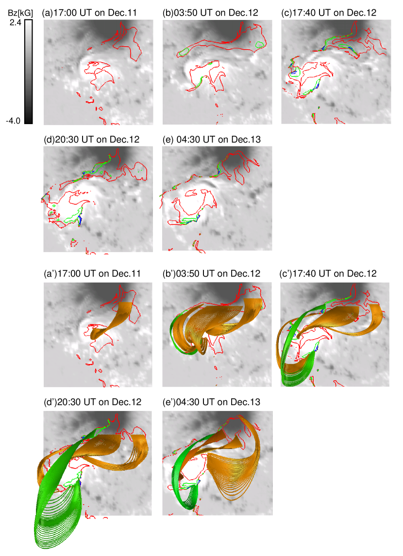
Figure 2: Upper panels(a$-$e): temporal evolution of selected twist magnitudes $|T_{n}|=0.5$, $|T_{n}|=1.0$, and $|T_{n}|=1.5$, plotted in red, green, and blue lines, respectively, over the normal component of the magnetic field in gray scale in the same field of view as Figure 1. Lower panels(a’$-$e’): selected magnetic field lines are also plotted. Orange and green field lines represent twist ranges of $0.5<|T_{n}|<1.0$ and $1.0<|T_{n}|<1.5$, respectively.

The magnetogram set on the bottom boundary is a hybrid map from SOT/Hinode and the Michelson Doppler Imager (MDI) on the Solar and Heliospheric Observatory (SOHO) (Scherrer et al. 1995). To obtain an extensive overview of the numerical box (see Figure 2(a) in Inoue et al. 2012), the magnetogram from the spectropolarimeter (SP) on Hinode is located at the center of the MDI/SOHO data. The area outside of the region covered by the SP magnetogram is maintained by the longitudinal field of MDI/SOHO, whereas its tangential components are fixed by the potential field derived on the basis of a synoptic chart of the line-of-sight component of the magnetic field observed by MDI/SOHO. The lateral and upper boundary conditions are also fixed by the potential field components.

An initial condition is given by the potential field calculated from the normal component of the magnetic field on all the boundaries after satisfying $\int B_{n}dS=0$ in the entire domain, where $dS$ represents the surface element on all the boundaries, and the subscript n represents the component normal to the surfaces of the boundaries. The 3D configuration is shown in Figure 2(b) of Inoue et al. (2012). The velocity field $v$ set to zero on all the boundaries. A Neumann-type boundary condition ($\partial_{n}\phi=0$) is applied to the potential $\phi$ at all the boundaries, where $\partial_{n}$ represents the derivative along the normal direction on the surface.

The numerical scheme for this calculation is given by the Runge-Kutta-Gill scheme with fourth-order accuracy for the temporal integral and the central finite difference with second-order accuracy for the spatial derivative. The simulation domain is a rectangular box spanning $(0,0,0)<(x,y,z)<(4.0L_{0},4.4L_{0},2.2L_{0})$, which corresponds to $(295.2^{\prime\prime},324.6^{\prime\prime},162.3^{\prime\prime})$ in view angle. The domain is uniformly divided by a $128\times 128\times 64$ grid. The vector-field magnetogram located on the bottom boundary ($125\times 64$ grid) was formed by binning from the original magnetogram, which had a $1000\times 512$ grid.

2.2 Observations

We extrapolated the 3D force-free field of AR 10930 by using the vector magnetograms of an observation provided by the SP on SOT/Hinode. We used five magnetograms, which were observed at 17:00 UT on December 11; at 03:50 UT, 17:40 UT, and 20:30 UT on December 12; and at 04:30 UT on December 13, 2006. The first four data sets were taken before the onset of the X3.4-class flare, which occurred at 02:10 UT on December 13, 2006, whereas the last one was observed just after it. These data were obtained by Milne-Eddington inversion of the FeI lines at 630.15 nm and 630.25 nm. The minimum energy method was applied to solve the $180^{\circ}$ ambiguity (Metcalf 1994; Metcalf et al. 2006; Leka et al. 2009). We also compared the CaII H 3968 $\AA$ images with the 3D NLFFF. These images were provided by the Broadband Filter Imager (BFI) on SOT/Hinode, which has a time cadence of 2 min. The field of view is 223.15”$\times$111.58”, with a pixel size of about 0.109”. The CaII line is sensitive to temperature at $10^{4}$K, which corresponds to the lower chromosphere, and reacts strongly to chromospheric heating. In this study, the CaII images were employed from just after the flare onset to the growth phase of the two-ribbon structure, which corresponds to the time interval from 02:14 UT to 02:40 UT on December 13.

2.3 Analysis of the magnetic twist

We focus on the magnetic twist, which is defined as the turnover number of magnetic field lines in magnetic flux tubes and plays a key role in judging the stability or instability of a magnetic configuration, as mentioned in section 1. Although the detailed formulation and its implementation in terms of the results obtained from the NLFFF on AR 10930 using this magnetic twist are illustrated in our previous works, (e.g., Inoue et al. 2011 and Inoue et al. 2012), we briefly describe this key issue again here to refresh readers memories.

The magnetic twist ($T_{n}$) is related to the magnetic helicity; e.g., the helicity of a closed flux tube anchored on the solar surface is described by the following equation ( Berger & Field 1984; Moffatt & Ricca 1992; Berger & Prior 2006),

$$H=(T_{n}+W_{r}){\Phi}^{2},$$ (7)

where H, $\Phi$, and $W_{r}$ are the magnetic helicity, magnetic flux of a cross section of the flux tube, and magnetic writhe corresponding to the helical structure of an axis of the field line, respectively. $T_{n}$ indicates how much of the magnetic helicity is generated by the currents parallel to the flux tube axes $J_{||}$; thus, $T_{n}$ is described by

$$T_{n}=\int\frac{dT_{n}}{ds}ds=\int\frac{J_{||}}{4\pi B_{||}}ds,$$ (8)

where $||$ indicates the component parallel to the field line, and the line integral $\int ds$ is taken along the central magnetic field line of the flux tube (Berger & Prior 2006; Török et al. 2010).

In this study, because we assume the force-free state and calculate $T_{n}$ for each field line, the twist value can be replaced by

$$T_{n}=\frac{1}{4\pi}\int\alpha dl=\frac{1}{4\pi}\alpha L,$$ (9)

where $\alpha$ is the force-free $\alpha$ given in equation (1), the line integral $\int dl$ is taken along the magnetic field line, and $L$ represents the field line length.

We introduce the average force-free $\alpha$, which is defined as

$$\bar{\alpha}=\frac{1}{2}(\alpha_{+}+\alpha_{-}),$$ (10)

where $\alpha_{+}$ and $\alpha_{-}$ indicate the force-free $\alpha$ on the footpoints of each field line on the positive and negative polarities, respectively. This formulation is adopted to minimize the deviation of the force-free condition in the photosphere. Consequently, the twist is formulated in this study as

$$T_{n}=\frac{1}{4\pi}\bar{\alpha}L.$$ (11)

Before calculating the average force-free $\alpha$ ($\bar{\alpha}$), we first focus on those specific magnetic fields for which the normal component exceeds 30 G in order to avoid numerical errors; further, $\alpha=0$ is assumed for the rest of the area. Next, we average $\alpha$ over $3\times 3$ cells, and finally we obtain the average force-free $\alpha$ ($\bar{\alpha}$) after calculating $\alpha_{+}$ and $\alpha_{-}$.

Note that we should use this formulation of the twist with caution, as given in equations (8) or (9). Because its value also depends on the field line length, one would obtain very large values corresponding to the very long field lines that have one footpoint outside the AR. However, in this study we do not consider such long field lines and essentially restrict our analysis to closed field lines, using the original definition in which the footpoints of the magnetic field lines are anchored somewhere inside the AR, and the magnetic twist is considered as being effectively propagated along the field lines through the strong shearing and twisting motions of the sunspot.

3 Results

3.1 3D structure of the Solar Active Region 10930

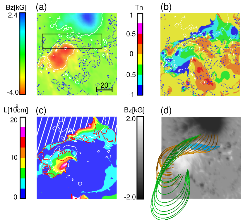
Figure 1: (a) Distribution of the normal component of the magnetic field ($B_{z}$) on the photosphere at 20:30 UT on December 12 (6 h before the flare). White solid lines indicate selected contours of $B_{z}$ (=790 G and $-$790 G); blue dotted lines are the PIL. Black solid square indicates the region near the PIL between the positive and negative polarities. (b) Twist ($T_{n}$) distribution of the field lines from NLFFF at 20:30 UT on December 12 mapped on the photosphere with the same white and blue contours as in (a). Positive and negative signs represent the distributions of right- and left-handed twisted lines, respectively. (c) Field line length mapped on the photosphere. Thin white lines have the same meaning as in (a); thick white diagonal lines indicate the region occupied by the open field lines that are connected outside the field of view. Red lines indicate a twist magnitude of $|T_{n}|=0.5$; i.e., the regions surrounded by red lines represent $|T_{n}|>0.5$. (d) Selected field lines plotted over the $B_{z}$ distribution. Blue, orange, and green field lines correspond to twist ranges of $|T_{n}|<$0.5, 0.5$<|T_{n}|<$1.0, and $|T_{n}|>$1.0, respectively. All panels(a$-$d) have the same field of view.

First, we try to understand the characteristics of the 3D magnetic structure 6 h before the flare associated with AR 10930 using twist analysis. The choice of this time is obvious because the vector field in its final pre-flare phase was observed around this time. The details of the force-freeness of the extrapolated fields were given in our previous work, Inoue et al. (2012). Figure 1(a) shows the distribution of the normal component of the magnetic field with the selected contours in white solid lines corresponding to $B_{z}$ = 790 G and $-$790 G, whereas the blue dotted lines correspond to the PIL. The black solid square box indicates the region surrounding the PIL between the positive and negative polarities of the sunspot.

Figure 1(b) represents the twist distribution of the field lines of the NLFFF mapped on the photosphere in the same field of view as in Figure 1(a), where the white solid and blue dotted lines have the same meaning. Note that these twisted values are focused on closed field lines only, as mentioned in subsection 2.3. The positive and negative twist distributions describe right- and left-handed field line twists, respectively. A strong negative twist ($|T_{n}|>0.5$) is clearly distributed on both sunspots; the strongest twisted region (more than one turn) also appears here. Hereafter, “strong twisted lines” usually refers to field lines having more than a half-turn twist ($|T_{n}|>0.5$). From this result, it is evident that the energy accumulated field lines are connected mainly between these strong twisted regions, which are at a considerable distance from the PIL. On the other hand, the region near the PIL surrounded by the black solid square in Figure 1(a) is of mixed polarity, containing both positively and negatively twisted field lines. However, the magnitudes of the twist values are much smaller ($|T_{n}|<0.25$) than those of the outer field lines characterized by strong negative twist that occupy the main twisted region of both polarities

Figure 1(c) shows the field line length ($L$) mapped on the photosphere in the same field of view as Figure 1(a), where the regions surrounded by red lines correspond to a twist value of $|T_{n}|>0.5$. The region marked by diagonal lines is occupied by open field lines that are connected outside the field of view. The mixed region of positively and negatively twisted field lines near the PIL enclosed by the solid square in Figure 1(a) consists of shorter magnetic field lines compared to the strongly twisted region surrounded by the red contours. From these results, AR 10930 can be roughly divided into two regions. One is occupied by the strongly negatively twisted field lines of single magnetic helicity and is located at a considerable distance from the PIL. The other corresponds to a mixed region of both positively and negatively twisted field lines near the PIL between the positive and negative polarities of the sunspot.

A 3D representation of the magnetic field lines is shown in Figure 1(d), which covers the same field of view as Figure 1(a). The blue, orange, and green field lines represent selected 3D magnetic field lines having twist values of $|T_{n}|<0.5$, $0.5<|T_{n}|<1.0$, and $1.0<|T_{n}|<1.5$, respectively. The orange and green lines are clearly longer than the blue one. On the other hand, the magnetic shear corresponding to the blue lines is stronger than that of the other field lines despite its weaker twist strength. This will be discussed in more detail in a later section.

3.2 An Evolution of the Magnetic Twist in the Solar Active Region 10930

3.2.1 An Evolution of the Strong Twisted field Lines Forming at a Considerable Distance from the PIL

In the previous section, we investigated the 3D magnetic structure of AR NOAA 10930 6 h before the flare. Here, we investigate the temporal evolution of the magnetic twist associated with this AR using the NLFFF derived from the time series of the vector fields taken before and after the flare. In the upper panels of Figure 2(a$-$e), the temporal evolution of twist having three different values, $|T_{n}|=0.5$, $|T_{n}|=1.0$, and $|T_{n}|=1.5$, is plotted in red, green, and blue contours, respectively, over the normal component of the magnetic field, represented in gray scale. The field of view is the same as in Figure 1. In the lower panels (a’$-$e’), the orange and green lines represent selected 3D magnetic field lines having twist strengths of $0.5<|T_{n}|<1.0$ and $1.0<|T_{n}|<1.5$, respectively.

At 17:00 UT on December 11, the strong twist ($|T_{n}|>0.5$) was distributed on the positive sunspot and the southwest edge of the negative sunspot. It was built up by the counterclockwise motion of the positive sunspot, as mentioned in section 1. The strongly twisted regions are connected with orange field lines, as shown in the Figure 2(a’). At 03:50 UT on December 12, the twist distribution grew wider, and in some regions, even stronger twist (more than one turn) can be seen. A comparison of the twist analysis at three different times before the flare, 03:50 UT, 17:40 UT, and 20:30 UT on December 12, reveals that the regions having a twist of more than one turn were spreading more at both polarities, and some magnetic lines with strong twist appear in the expansion stage owing to the continuous shearing and twisting motions of the positive sunspot. Figure 2(d), obtained 6 h before the flare, is the final picture of the magnetic configuration in the pre-flare phase. Although the strongly twisted lines ($|T_{n}|>1.0$) are widely distributed compared to the previous times, they are localized on the edge of the sunspot, where the magnetic field strength is weaker than at the central part of the sunspot. The post-flare image, Figure 2(e), corresponds to 2 h after flare onset. The twisted field lines decrease, which is also reported for another AR in a recent paper Sun et al. (2012), in the central part of the positive sunspot, which consisted mainly of field lines of twist $|T_{n}|<1.0$ before the flare. However, the part of the strong twist confined at the edge of the positive sunspot remained even after the flare.

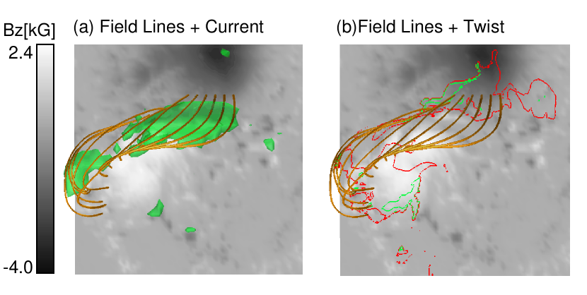
Figure 3: Magnetic field lines and surface having strong current density ($|J|>$ 2.4) at 20:30 UT on December 12 (orange and green, respectively) over the normal component of the magnetic field (gray scale) in the same field of view as Figure 1. (b) Twist distributions in red ($|T_{n}|=0.5$) and green ($|T_{n}|=1.0$) contours with the field lines as in (a).

From these analyses, we infer that although the positive sunspot is capable of generating strongly twisted lines of more than half a turn in the energy accumulation process because of its strong twisting and shearing motions, the strongest twist (in particular, $|T_{n}|>1.0$) does not seem to contribute efficiently to the main energy release. To further investigate this point, let us examine the distribution of the current density along the twisted field lines. An estimation of the strong current density, which is related to the measurement of a large free energy through the twisted field lines, would provide a way to clarify whether the most strongly twisted lines ($|T_{n}|>1.0$) are capable of causing X-class flares. Figure 3(a) shows the field lines in orange with the strong current density region represented by the green surface over the normal component of the magnetic field in gray scale at 20:30 UT on December 12. Because these field lines surround the surface of the strong current density region, they are expected to store considerable free energy. Figure 3(b) represents the twist distribution by red ($|T_{n}|=0.5$) and green ($|T_{n}|=1.0$) contours mapped on the photosphere, with the same field lines as in Figure 3(a). The footpoints of most field lines are clearly rooted in the regions surrounded by the red contours, which clarifies that the twist values of the field lines supporting the strong current density are distributed in the range of $0.5<|T_{n}|<1.0$. Hence, these results suggest that the field lines having a twist of more than one turn could not be deeply connected with the release of free energy in X-class flares.

3.2.2 An Evolution of the Twisted Lines Near the Polarity Inversion Lines

In this subsection, we present the temporal evolution of the magnetic twist near the PIL. Because many flares are observed to originate at the PIL, it becomes imperative to observe the behavior of the magnetic twist near this region. The left panels in Figure 4 shows the temporal evolution of the twist distribution near the PIL. Blue and red lines indicate the locations of the negative and positive sunspots, respectively, which are defined as in Figure 1. The green lines represent the PIL. The black and white areas represent the negatively and positively twisted regions occupied by closed field lines, whereas the regions occupied by open field lines are shown in gray and are outside the scope of discussion in this study. At 17:00 UT on December 11, this active region consisted almost entirely of field lines having negative twist values. The positive sunspot’s motion had already developed this twisted region more than a day before flare onset. The positively twisted regions gradually increased as the flare onset approached. Finally, after the flare, most regions near the PIL between the positive and negative sunspots were occupied by positively twisted field lines. The time evolution of field lines in this AR is characterized mainly by the negatively twisted field due to the positive sunspot’s motion (Figure 2). However, positive twist begins to buildup at 03:50 UT on December 12, about one day before flare onset, and it formed in less time than the strongly negatively twisted regions. This result is consistent with Park et al. (2010), which describes the injection of positive helicity into a pre-existing system having negative helicity on a shorter time scale. Recently, Ravindra et al. (2011) also showed the injection of an opposite vertical current near the PIL through the net current distribution on both polarities.

We also check the average force-free $\alpha$, denoted as $\bar{\alpha}$. The color map in the right panels in Figure 4 shows the temporal evolution of $\bar{\alpha}$. Its pattern is also very similar to that of the twisted field lines shown in the left panels. The negative $\bar{\alpha}$ is already injected in the early phase, whereas the positive $\bar{\alpha}$ increases gradually near the PIL as time proceeds. Unlike the twist distribution, some of the positive $\bar{\alpha}$, for example, the region surrounded by the solid square in the right panels, is comparable in strength to the negative $\bar{\alpha}$, although the magnitudes of the positive twist values are much smaller than those in the negative $\bar{\alpha}$ regions (see Figure 1(b)). Consequently, we see a much different picture in terms of the twist analysis.

3.3 Release Process of the Magnetic Twist in the X3.4 Class Flare Occurred in the Solar Active Region 10930

3.3.1 Twist distribution vs. Evolution of the Flare Ribbon

Here, we investigate the release process of the magnetic twist before and after the flare in detail in order to understand the flare dynamics in terms of the variations in the twist value. First, we check the temporal evolution of the CaII illumination obtained from SOT/Hinode and compare it with the magnetic twist obtained through the NLFFF to clarify the relationship between them.

The gray scale map in Figure 5 shows running difference images of CaII from 02:14 UT to 02:24 UT on December 13. This time period corresponds to the growth phase of the two-ribbon structure. The white solid and dashed lines represent the locations of the positive and negative sunspots at 20:30 UT on December 12, which are defined as in Figure 1. At the initial onset phase, around 02:14 UT on December 13, the CaII image shows strong illumination around the local area nearby the PIL, which is surrounded by the white dotted square. The two-ribbon structure had still not formed at this time. A thin two-ribbon structure started to form around 02:18 UT on December 13 and finally became thick and showed strong illumination from 02:22 UT to 02:24 UT on December 13.

Figure 5 shows contours corresponding to the twist value $|T_{n}|=0.5$ (red lines), which were obtained from the NLFFF at 20:30 UT on December 12. The regions surrounded by the red lines are occupied by strongly twisted field lines (greater than a half-turn twist, i.e., $|T_{n}|>0.5$). The initial illumination at 02:14 UT on December 13 clearly comes from the weakly twisted region where $|T_{n}|<$ 0.25. Although the initial two-ribbon structure at 02:18 UT on December 13 formed in the weakly twisted region, it seems to be associated with strong illumination in the later stage (02:22 UT and 02:24 UT on December 13) in the strongly twisted region. From this result, we infer that the strong CaII illumination seems to be related to the strongly twisted magnetic fields.

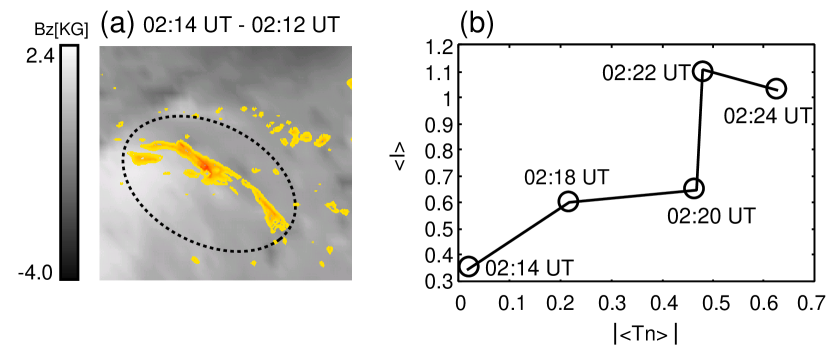
Figure 6: (a) Areas of strong CaII intensity ($I>$150, filled contours) at 02:14 UT on December 13 plotted on a distribution map of the normal component of the magnetic field (gray scale) at 20:30 UT on December 12. Image covers the area enclosed by the dotted square in Figure 5(a). Northern and southern ribbons cannot be distinguished at this time because the two-ribbon structure had not formed yet, as shown in Figure 5. (b) Profile of $\langle I\rangle$, normalized by the $\langle I\rangle$ = 1000, as a function of $|\langle T_{n}\rangle|$ at various times on December 13.

We further investigate the relationship between the CaII intensity and magnetic twist value more quantitatively. We define the average CaII intensity $\langle I\rangle$ and average twist value $|\langle T_{n}\rangle|$. The CaII intensities are also based on the running difference images, as shown in Figure 6. Here “average” indicates the average intensity in the northern ribbon, where only the region of strong CaII illumination is selected by setting the threshold value of the CaII intensity to $I$ = 200. However, because the two-ribbon structure had not formed at 02:14 UT on December 13, we cannot distinguish the northern and southern ribbons. Hence, we need to calculate these average intensities using another path instead of the northern ribbon. Figure 6(a) shows the area surrounded by the dotted square in Figure 5(a); the strong CaII intensity (filled contours at $I>$ 150) at 02:14 UT on December 13 is plotted on a distribution map of the normal component of the magnetic field (gray scale) at 20:30 UT on December 12. At this time only, $\langle I\rangle$ and $|\langle T_{n}\rangle|$ were calculated for the strong CaII intensity region surrounded by a dotted circle in Figure 6(a). Figure 6(b) shows the profile of $\langle I\rangle$, which is normalized by the $\langle I\rangle$ = 1000, as a function of $|\langle T_{n}\rangle|$. This result clearly shows that $\langle I\rangle$ suddenly increased for $|\langle T_{n}\rangle|$ = 0.47 at 02:22 UT on December 13, which indicates that a dramatic reconnection occurred in the magnetic twist having values of $|\langle T_{n}\rangle|>0.47$ because strong CaII illumination is strongly correlated with magnetic reconnection (Priest & Forbes 2002). From these results, we find that the strong twist has a significant relationship with the strong CaII intensity.

Note that this conclusion is not inconsistent with our previous finding (Inoue et al. (2012)), in which we showed that strong X-ray intensity is not related to strongly twisted lines but rather shows a good correlation with the field-aligned current. Our previous study examined the core region of the sigmoid, which consisted of weakly twisted field lines and was located inside the strongly twisted field lines forming the elbow part of the sigmoid and revealing strong CaII intensity. Therefore, the environment of the magnetic field lines making up the core of the sigmoid differs from the environment we discuss in this work.

3.3.2 Relaxation of the Magnetic Twist through the Flare

We proceed with a detailed investigation of the changes in the magnetic topology due to magnetic reconnection before and after the flare by using the magnetic twist obtained through the NLFFF and CaII images. Figures 7(a) and (b) show the magnetic field lines (in gray) before and after the flare over a time integration of the CaII images from 02:20 UT to 02:40 UT on December 13, that is, from the growth to the formation of the two-ribbon flare structure. The regions surrounded by red lines, labeled R1 and R2 or R1’ and R2’, are occupied by closed strongly twisted lines ($|T_{n}|>0.5$) from the NLFFF (a) before and (b) after the flare (20:30 UT on December 12 and 04:30 UT on December 13, respectively). Selected magnetic field lines, labeled L1 (L1’) and L2 (L2’) connect the strongly twisted regions R1 (R1’) and R2 (R2’) before (after) the flare. Note that although L1 (or L2) and L1’ (or L2’) are plotted for the same location, there is no similarity among them.

The strongly twisted regions R1 and R2 before the flare are clearly located in the area where the CaII image showed brightening, some parts of which disappeared after the flare even though regions R1’ and R2’ remained as such. In the region where the strong twist disappeared, the selected magnetic fluxes L1’ and L2’ seemed to relax into an untwisted field relative to L1 and L2. In particular, the field line L1 forms a compact loop, as shown in Sun et al. (2012). Because this relaxation appears on the image of the strong CaII illumination, magnetic reconnection may be a candidate for explaining the relaxation of the magnetic twist.

Figures 7(c) and (d) show scatter plots of the twist $T_{n}$ (vertical axis) vs. the normal component of the magnetic field $B_{z}$ (horizontal axis) before and after the flare, respectively. Negatively twisted lines are distributed over a wide range of the normal component of the magnetic field. Dashed circles A and B indicate the strong negatively twisted regions in the negative and positive polarities, respectively, before the flare. Many of the points in regions A and B before the flare clearly disappeared after the flare, although some remained. The twisted field lines representing $T_{n}\approx-0.5$ seem to still be distributed over a wide range of the normal component of the magnetic field after the flare. Therefore, we suggest that most of the twist release is caused by field lines with at least $T_{n}<-0.5$. On the other hand, the positively twisted regions marked by dashed circle C appear for $|B_{z}|<0.2$ before the flare and remain as such even after the flare. From this result, we clearly see again that the mixed region indicating coexistence of the negatively and positively twisted lines is formed at $|B_{z}|<0.2$, as shown in the left panels in Figure 4.

4 Discussion

In the previous section, we discussed the buildup and release processes of the magnetic twist through the huge X-class flare associated with AR 10930. Here, we address a possible mechanism for the onset of this flare.

The above results (Figures 5 - 7) showed that energy is released mainly by magnetic reconnection of the field lines having a strong negative twist. However, we still have not answered the question regarding the flare onset mechanism that we posed at the beginning of the paper. Figure 5(a) shows that flare onset starts at around 02:14 UT between the positive and negative polarities of the sunspot, where weakly twisted lines ($|T_{n}|<0.25$) appear near the PIL. Because this region is also composed of a mixture of field lines having both positive and negative twist, magnetic reconnection may be easily induced between lines having opposite twist. The mixed-twist region was able to form because positively twisted field lines were injected across the pre-existing negatively twisted lines.

Further, we investigate the temporal evolution of the magnetic flux corresponding to the positive twist and compare it with that of the magnetic flux corresponding to the negative twist. Figure 8 shows the temporal evolution of the magnetic flux, log ($\Phi$) ($B_{z}>0$), for $T_{n}<-0.5$ and $T_{n}>0$, which are represented by solid and dashed lines, respectively, corresponding to the areas displayed in Figures 2 and 4, respectively. The vertical dashed line indicates the flare onset time. We found that most of the magnetic twist producing the flare was greater than a half-turn in the negative sense ($T_{n}<-0.5$). The time profiles of both magnetic fluxes show an increase as the flare onset time approached. However, the magnetic flux related to $T_{n}<-0.5$ decreased dramatically around the flare onset time. We believe that this decrement in the magnetic flux related to the negative twist is due to the relaxation via magnetic reconnection shown in Figures 5-7. In contrast, the magnetic flux corresponding to $T_{n}>0$ increased continuously before and after flare onset.

In previous studies, Inoue et al. (2011) and Inoue et al. (2012) indicated that the magnetic configuration occupying the strongly twisted regions before the flare was robust against kink mode instability; therefore, this AR cannot be destabilized through kink instability. Hence, flare onset is triggered via another mechanism: breaking of the equilibrium condition of the strongly twisted field; the buildup of positive twist may be a candidate cause of that collapse. Consequently, we can say that the increase in the magnetic flux due to injection of twist of the opposite sign across the pre-existing field is an important process for understanding the flare trigger mechanism.

We again look at the distribution maps of the twisted and average force-free $\alpha$ (denoted as $\bar{\alpha}$) at 20:30 UT on December 12 in the left and right panels in Figures 4. Although the twist value in the mixed-sign region marked by the black square in Figure 1(a) is weak relative to the negative twist values distributed at a considerable distance from the PIL (Figure 1(b)), the strong $\bar{\alpha}$ is injected into the region occupied by this weak mixed-sign field (for example, the region surrounded by the solid square in the right panels in Figure 4). The twist value is small in this region because it depends strongly on the field line length, even though strong force-free $\alpha$ exists at their footpoints. Pevtsov et al. (1997) reported a strong correlation between the force-free $\alpha$ and the geometric shear angle $\theta$ (equation (5.3.18) in Aschwanden 2004) from the soft X-ray loops observed by the Soft X-Ray Telescope (SXT) on Yohkoh. Therefore, this result implies that the buildup of strong magnetic shear of opposite sign may be related to flare onset, even though the field lines are extremely short (see Figure 1(c)). However, we cannot identify the essential process related to the amount of positively twisted magnetic flux or the strength of the average force-free $\alpha$. We need further statistical analysis using data with a higher time cadence or numerical experiments to answer this question.

Some authors have already proposed theoretical flare/CME models in which small-scale reconnection in the local area at the lower corona leads to large-scale reconnection, releasing the magnetic energy. In a 2D model, Chen & Shibata (2000) and Shiota et al. (2005) successfully interpreted an eruption as magnetic reconnection between the emerging flux and the pre-existing magnetic flux, which leads to a loss of equilibrium in the flux tube; subsequently, another magnetic reconnection is induced in the pre-existing lines under the eruptive flux rope.

On the other hand, Kusano et al. (2004) conducted a 3D simulation to determine the role of local instability to determine whether it leads to an ejective eruption. They reported that tearing instability occurs at the lower corona where the reversed magnetic shear field is formed against the overlying field and eventually leads to ejective eruption through a nonlinear feedback process, that is the mutual interaction between large-scale strongly twisted lines and a small-scale region of mixed twist (Kusano et al. 2004 ). They also proposed that the key process of flare onset is magnetic reconnection between field lines having different twist in the local area of the lower corona, which becomes an important cause of large-scale flares. Thus, our result shows behavior similar to that of the theoretical model proposed by Kusano et al. (2004). However, it is much difficult to conclude an answer of the onset mechanism in term of the only quasi-static pictures obtained from NLFFF.

Although we suggest that the formation of two different regions is important for flare onset, the detailed formation process is still not well known. Nevertheless, Park et al. (2010), Ravindra et al. (2011), and Ravindra et al. (2011) recently suggested that the process of building up positively twisted lines over pre-existing negatively twisted lines seems to be a possible component of the flare onset mechanism. Wang et al. (2008) and Lim et al. (2010) indicated that flux emergence is a key process in the formation of these structures and is also responsible for flare onset. The key problems are how the mixed-helicity region is formed on the local area near the PIL and how it plays a key role in exciting a flare. A flux emergence simulation may address these questions in the future.

5 Summary

In this paper, we investigated the temporal evolution of the 3D magnetic structure of AR 10930. We examined the buildup and release processes of the magnetic twist associated with this AR using a time series of the vector fields before and after a flare. Our analysis is based on the NLFFF extrapolation method, which is applied to time series data obtained from SP/Hinode. We also suggested a possible flare onset mechanism in terms of magnetic reconnection between field lines having opposite twist.

We found that the 3D magnetic structure of this AR can be roughly separated into two regions containing field lines having different twist. One is occupied by field lines of strong negative twist, (i.e., left-handed twist) rooted in the regions of both polarities and is located at a considerable distance from the PIL. The other is of mixed polarity and contains both positively and negatively twisted lines near the PIL between two sunspots. We investigated the temporal evolution of the magnetic twist (i.e., from its buildup to its release) associated with this AR using time series NLFFF. We found that a day before flare onset, most regions were occupied by negatively twisted field lines. Positively twisted lines were also built up near the PIL within one day; consequently, the mixed region was formed, which was eventually occupied and dominated by positively twisted lines after the flare.

For flare onset, we suggest the importance of the buildup near the PIL of twisted magnetic lines of different sign compared to the ambient field. In this situation, magnetic reconnection can be induced between field lines having different twist, which would destroy the equilibrium of the magnetic configuration. We also found that the main relaxation process in the flare dynamics is caused by magnetic reconnection in strongly negatively twisted lines by comparing CaII images with the NLFFF. This scenario is similar to a previous model proposed by Kusano et al. (2004). Unfortunately, we cannot extract much more information from the NLFFF and conclude a clear answer for the onset mechanism because it is useful for magnetic structures in a quasi-static state. Thus, we still have problems such as the transition process from a stable condition to an unstable or non-equilibrium condition and the 3D dynamics of magnetic reconnection in the solar corona. We believe that MHD simulations may provide strong clues regarding these points.

In addition, this study is essentially limited by the low time cadence of the SP data ($\sim$10 h) used in this analysis. To achieve a more comprehensive view of the temporal evolution of the 3D magnetic structure, high-cadence data are essential. A new solar physics satellite, Solar Dynamics Observatory (SDO) was launched recently by the National Aeronautics and Space Administration (NASA). The Helioseismic and Magnetic Imager (HMI) on board SDO can provide vector magnetograms with higher time cadence and a larger field of view compared to the data obtained from Hinode. The detailed time evolution of the magnetic field lines and accurate reproduction of the location of the separatrix are important issues for the understanding of the flare onset and dynamics. We will deepen our understanding of the onset of solar flares by combining high temporal resolution data from SDO with high spatial resolution data obtained by Hinode.

Figure 4: Left panels; Positive and negative twist distributions for closed loops plotted in white and black, respectively. Gray regions are occupied by open field lines. Red and blue lines indicate the locations of the positive and negative sunspots, respectively, which correspond to a normal component of the magnetic field of 790 G and $-$790 G, respectively. Dotted green lines indicate the PIL. Right panels; Average force-free $\alpha$, denoted by $\bar{\alpha}$, plotted in color. White solid lines indicate positive and negative polarities; white dotted line represents the PIL, which is also shown in (a).

Figure 5: (a)-(d) Gray scale maps showing the temporal evolution of CaII images, which are running difference images, corresponding to growth of the flare ribbon in the early phase of the flare (02:14 UT to 02:24 UT on December 13). The field of view is the same as in Figure 1. Red lines indicate contours of twist $|T_{n}|=0.5$ obtained from the NLFFF at 20:30 UT on December 12. White solid and dashed lines represent contours of the normal component of the magnetic field, defined as in Figure 1(a). Dotted square suggests the location of illumination corresponding to the flare onset.

Figure 7: Color maps of time integration of CaII images from 02:20 UT to 02:40 UT on December 13. Red lines represent twist values of $|T_{n}|$ = 0.5 from the NLFFF at (a) 20:30 UT on December 12 (before the flare) and (b) 04:30 UT on December 13 (after the flare). R1 (R1’) and R2 (R2’) represent the strongly twisted regions ($|T_{n}|>$0.5) on the negative and positive polarities, respectively. L1 (L1’) and L2 (L2’) are selected magnetic field lines connecting R1 (R1’) and R2 (R2’). (c) and (d) Scatter plots of twist $T_{n}$ (vertical axis) vs. $B_{z}$ (horizontal axis) before and after the flare, respectively. Dashed circles A and B in (c) show the regions where the strong twist was distributed before the flare. Region C represents the positively twisted region of approximately $|B_{z}|<$ 0.2 before the flare.

Figure 8: Temporal evolution of the magnetic flux, log($\Phi$) ($B_{z}>0$), for $T_{n}>0$ (dashed line) and $T_{n}<-0.5$ (solid line), respectively, corresponding to the areas displayed in Figures 2 and 4, respectively. These values are normalized by $10^{24}$ (Mx) (=$\int B_{0}dS$; $dS$ represents an surface element in the bottom surface). Vertical dashed line indicates the time at which the flare occurred.

References

- Aschwanden (2004) Aschwanden, M. J. 2004, Physics of the Solar Corona,
- Berger & Field (1984) Berger, M. A., & Field, G. B. 1984, Journal of Fluid Mechanics, 147, 133
- Berger & Prior (2006) Berger, M. A., & Prior, C. 2006, Journal of Physics A Mathematical General, 39, 8321
- Chen & Shibata (2000) Chen, P. F., & Shibata, K. 2000, ApJ, 545, 524
- Chen (2011) Chen, P. F. 2011, Living Reviews in Solar Physics, 8, 1
- Dedner et al. (2002) Dedner, A., Kemm, F., Kröner, D., Munz, C.-D., Schnitzer, T., & Wesenberg, M. 2002, Journal of Computational Physics, 175, 645
- Demoulin et al. (1996) Demoulin, P., Henoux, J. C., Priest, E. R., & Mandrini, C. H. 1996, A&A, 308, 643
- Forbes (1990) Forbes, T. G. 1990, J. Geophys. Res., 951, 11919
- Guo et al. (2008) Guo, Y., Ding, M. D., Wiegelmann, T., & Li, H. 2008, ApJ, 679, 1629
- He et al. (2011) He, H., Wang, H., & Yan, Y. 2011, Journal of Geophysical Research (Space Physics), 116, 1101
- Inoue & Kusano (2006) Inoue, S., & Kusano, K. 2006, ApJ, 645, 742
- Inoue et al. (2008) Inoue, S., Kusano, K., Masuda, S., et al. 2008, First Results From Hinode, 397, 110
- Inoue et al. (2011) Inoue, S., Kusano, K., Magara, T., Shiota, D., & Yamamoto, T. T. 2011, ApJ, 738, 161
- Inoue et al. (2012) Inoue, S., Magara, T., Watari., & Choe, G. S. 2012, ApJ, 747, 65
- Isenberg et al. (1993) Isenberg, P. A., Forbes, T. G., & Demoulin, P. 1993, ApJ, 417, 368
- Jing et al. (2008) Jing, J., Chae, J., & Wang, H. 2008, ApJ, 672, L73
- Jing et al. (2008) Jing, J., Wiegelmann, T., Suematsu, Y., Kubo, M., & Wang, H. 2008, ApJ, 676, L81
- Kataoka et al. (2009) Kataoka, R., Ebisuzaki, T., Kusano, K., et al. 2009, Journal of Geophysical Research (Space Physics), 114, 10102
- Kosugi et al. (2007) Kosugi, T., et al. 2007, Sol. Phys., 243, 3
- Kubo et al. (2007) Kubo, M., et al. 2007, PASJ, 59, 779
- Kruskal & Kulsrud (1958) Kruskal, M. D., & Kulsrud, R. M. 1958, Physics of Fluids, 1, 265
- Kusano et al. (2004) Kusano, K., Maeshiro, T., Yokoyama, T., & Sakurai, T. 2004, ApJ, 610, 537
- Leka et al. (2009) Leka, K. D., Barnes, G., & Crouch, A. 2009, Astronomical Society of the Pacific Conference Series, 415, 365
- Lim et al. (2010) Lim, E.-K., Chae, J., Jing, J., Wang, H., & Wiegelmann, T. 2010, ApJ, 719, 403
- Liu et al. (2008) Liu, Y., Luhmann, J. G., Müller-Mellin, R., et al. 2008, ApJ, 689, 563
- Magara (2004) Magara, T. 2004, ApJ, 605, 480
- Magara & Tsuneta (2008) Magara, T., & Tsuneta, S. 2008, PASJ, 60, 1181
- Metcalf (1994) Metcalf, T. R. 1994, Sol. Phys., 155, 235
- Metcalf et al. (2006) Metcalf, T. R., Leka, K. D., Barnes, G., et al. 2006, Sol. Phys., 237, 267
- Metcalf et al. (2008) Metcalf, T. R., et al. 2008, Sol. Phys., 247, 269
- Min & Chae (2009) Min, S., & Chae, J. 2009, Sol. Phys., 258, 203
- Moffatt & Ricca (1992) Moffatt, H. K., & Ricca, R. L. 1992, Royal Society of London Proceedings Series A, 439, 411
- Park et al. (2010) Park, S.-H., Chae, J., Jing, J., Tan, C., & Wang, H. 2010, ApJ, 720, 1102
- Pevtsov et al. (1997) Pevtsov, A. A., Canfield, R. C., & McClymont, A. N. 1997, ApJ, 481, 973
- Priest & Forbes (2002) Priest, E. R., & Forbes, T. G. 2002, A&A Rev., 10, 313
- Ravindra et al. (2011) Ravindra, B., Venkatakrishnan, P., Tiwari, S. K., & Bhattacharyya, R. 2011, ApJ, 740, 19
- Ravindra et al. (2011) Ravindra, B., Yoshimura, K., & Dasso, S. 2011, ApJ, 743, 33
- Savcheva & van Ballegooijen (2009) Savcheva, A., & van Ballegooijen, A. 2009, ApJ, 703, 1766
- Scherrer et al. (1995) Scherrer, P. H., Bogart, R. S., Bush, R. I., et al. 1995, Sol. Phys., 162, 129
- Schrijver et al. (2008) Schrijver, C. J., et al. 2008, ApJ, 675, 1637
- Shibata & Magara (2011) Shibata, K., & Magara, T. 2011, Living Reviews in Solar Physics, 8, 6
- Shiota et al. (2005) Shiota, D., Isobe, H., Chen, P. F., Yamamoto, T. T., Sakajiri, T., & Shibata, K. 2005, ApJ, 634, 663
- Su et al. (2007) Su, Y., et al. 2007, PASJ, 59, 785
- Su et al. (2009) Su, J. T., Sakurai, T., Suematsu, Y., Hagino, M., & Liu, Y. 2009, ApJ, 697, L103
- Su et al. (2009) Su, Y., van Ballegooijen, A., Lites, B. W., Deluca, E. E., Golub, L., Grigis, P. C., Huang, G., & Ji, H. 2009, ApJ, 691, 105
- Sun et al. (2012) Sun, X., Hoeksema, J. T., Liu, Y., et al. 2012, ApJ, 748, 77
- Török et al. (2004) Török, T., Kliem, B., & Titov, V. S. 2004, A&A, 413, L27
- Török et al. (2010) Török, T., Berger, M. A., & Kliem, B. 2010, A&A, 516, A49
- Tsuneta et al. (2008) Tsuneta, S., Ichimoto, K., Katsukawa, Y., et al. 2008, Sol. Phys., 249, 167
- Wang et al. (2008) Wang, H., Jing, J., Tan, C., Wiegelmann, T., & Kubo, M. 2008, ApJ, 687, 658
- Zhang et al. (2007) Zhang, J., Li, L., & Song, Q. 2007, ApJ, 662, L35
- Zhang (2010) Zhang, H. 2010, ApJ, 716, 1493