People born in the Middle East but residing in the Netherlands: Invariant population size estimates and the role of active and passive covariates

Abstract

Including covariates in loglinear models of population registers improves population size estimates for two reasons. First, it is possible to take heterogeneity of inclusion probabilities over the levels of a covariate into account; and second, it allows subdivision of the estimated population by the levels of the covariates, giving insight into characteristics of individuals that are not included in any of the registers. The issue of whether or not marginalizing the full table of registers by covariates over one or more covariates leaves the estimated population size estimate invariant is intimately related to collapsibility of contingency tables [Biometrika 70 (1983) 567–578]. We show that, with information from two registers, population size invariance is equivalent to the simultaneous collapsibility of each margin consisting of one register and the covariates. We give a short path characterization of the loglinear model which describes when marginalizing over a covariate leads to different population size estimates. Covariates that are collapsible are called passive, to distinguish them from covariates that are not collapsible and are termed active. We make the case that it can be useful to include passive covariates within the estimation model, because they allow a finer description of the population in terms of these covariates. As an example we discuss the estimation of the population size of people born in the Middle East but residing in the Netherlands.

, , , and

1 Introduction

A well-known technique for estimating the size of a human population is to find two or more registers of this population, to link the individuals in the registers and to estimate the number of individuals that occur in neither of the registers [Fienberg (1972); Bishop, Fienberg and Holland (1975); Cormack (1989); International Working Group for Disease Monitoring and Forecasting, IWGDMF (1995)]. For example, with two registers $A$ and $B$, linkage gives a count of individuals in $A$ but not in $B$, a count of individuals in $B$ but not in $A$, and a count of individuals both in $A$ and $B$. The counts form a contingency table denoted by $A\times B$, with the variable labeled $A$ being short for “inclusion in register $A$” taking the levels “yes” and “no,” and likewise for register $B$. In this table the cell “no, no” has a zero count by definition, and the statistical problem is to better estimate this value in the population. An improved population size estimate is obtained by adding this estimated count of missed individuals to the counts of individuals found in at least one of the registers.

With two registers the usual assumptions under which a population size estimate is obtained are as follows: inclusion in register $A$ is independent of inclusion in register $B$; and in at least one of the two registers the inclusion probabilities are homogeneous [see Chao et al. (2001) and Zwane, van der Pal and van der Heijden (2004)]. Interestingly, it is often, but incorrectly, supposed that both inclusion probabilities have to be homogeneous. Other assumptions are that the population is closed and that it is possible to link the individuals in registers $A$ and $B$ perfectly.

However, it is generally agreed that these assumptions are unlikely to hold in human populations. Three approaches may be adopted to make the impact of possible violations less severe. One approach is to include covariates into the model, in particular, covariates whose levels have heterogeneous inclusion probabilities for both registers [see Bishop, Fienberg and Holland (1975); Baker (1990); compare Pollock (2002)]. Then loglinear models can be fitted to the higher-way contingency table of registers $A$ and $B$ and the covariates. The restrictive independence assumption is replaced by a less restrictive assumption of independence of $A$ and $B$ conditional on the covariates; and subpopulation size estimates are derived (one for every level of the covariates) that add up to a population size estimate. Another approach is to include a third register, and to analyze the three-way contingency table with loglinear models that may include one or more two-factor interactions, thus getting rid of the independence assumption. Here the (less stringent) assumption made is that the three-factor interaction is absent. However, including a third register is not always possible, as it is not available, or because there is no information that makes it possible to link the individuals in the third register to both the first and to the second register. A third approach makes use of a latent variable to take heterogeneity of inclusion probabilities into account [see Fienberg, Johnson and Junker (1999); Bartolucci and Forcina (2001)]. Of course, these three approaches are not exclusive and may be used concurrently in one model.

When the approach is adopted to use covariates, the question is which covariates should be chosen. In the traditional approach, only covariates that are available in each of the registers can be chosen. Recently, Zwane and van der Heijden (2007) showed that it is also possible to use covariates that are not available in each of the registers. For example, when a covariate is available in register $A$ but not in $B$, the values of the covariate missed by $B$ are estimated under a missing-at-random assumption [Little and Rubin (1987)]; and the subpopulation size estimates are then derived as a by-product. Whether or not the covariates are available in each of the registers, the number of possible loglinear models that can be fit grows rapidly.

In this paper we study the (in)variance of population size estimates derived from loglinear models that include covariates. Including covariates in loglinear models of population registers improves population size estimates for two reasons. First, it is possible to take heterogeneity of inclusion probabilities over the levels of a covariate into account; and second, it allows subdivision of the estimated population by the levels of the covariates, giving insight into characteristics of individuals that are not included in any of the registers. The issue of whether or not marginalizing the full table of registers by covariates over one or more covariates leaves the estimated population size estimate invariant is intimately related to collapsibility of contingency tables. With information from two registers it is shown that population size invariance is equivalent to the simultaneous collapsibility of each margin consisting of one register and the covariates. Covariates that are collapsible are called passive, to distinguish them from covariates that are not collapsible and are termed active. We make the case that it may be useful to include passive covariates within the estimation model, because they allow a description of the population in terms of these covariates. As an example we discuss the estimation of the population size of people born in the Middle East but residing in the Netherlands.

By focusing on population size estimates, collapsibility in loglinear models is studied in this paper from a different perspective than found in Bishop, Fienberg and Holland (1975) who are interested in parametric collapsibility. Our work applies model collapsibility of Asmussen and Edwards (1983), later discussed by Whittaker [(1990), pages 394–401] and Kim and Kim (2006), concerning the commutativity of model fitting and marginalization. We use model collapsibility in the context of population size invariance and show invariance requires model collapsibility of each margin consisting of one register and the covariates. A novel feature is to apply collapsibility in the context of a table containing structural zeros. We give a short path characterization of the loglinear model which describes when marginalizing over a covariate leads to different population size estimates.

The second result can be fruitfully applied in population size estimation. In a specific loglinear model, we denote covariates as passive when they are collapsible and active when they are not collapsible. In principle, the approach of Zwane and van der Heijden (2007) permits the inclusion of many passive covariates in a model; we make a case for including such passive covariates because they allow the description of both the observed part as well as the unobserved of the population in terms of these covariates.

The paper is built up as follows. In Section 2 we discuss the data to be analyzed. These refer to the population of people with Afghan, Iranian and Iraqi nationality residing in the Netherlands. In Section 3 we discuss theoretical properties of the loglinear models in the context of population size estimation. This is discussed in detail for the case of two registers. We illustrate the two properties of loglinear models using a number of examples, and then prove the properties using results from graphical models. We distinguish the standard situation that every covariate is available in each of the registers from the situation that there are one or more covariates that are available in only one of the registers [Zwane and van der Heijden (2007)]. For completeness we also discuss the situation when three registers are available and illustrate that the same properties apply. In Section 4 we develop the notion of active and passive covariates, and in Section 5 we present an example. We end with a discussion. In Appendix A we extend the work of Asmussen and Edwards (1983) to population size invariance.

2 The population of people with Middle Eastern nationality staying in the Netherlands

The preparations for the 2011 round of the Census are in progress at the time of writing. More countries now make use of administrative data (rather than polling) for that purpose. There are countries who are repeating this method, such as Denmark, Finland and the Netherlands, and more than ten European countries that are using administrative data for the first time [Valente (2010)]. The administrative registers are combined by data-linking and micro-integration to clean and improve consistency. The outcome of these processes is called a statistical register or a register for short.

The most important administrative register to be used in the Netherland Census is an automated system of decentralized (municipal) population registers (in Dutch, Gemeentelijke BasisAdminstratie, referred to by the abbreviation GBA). This register is used for the definition of the population. The GBA contains all information on people that are legally allowed to reside in the Netherlands and are registered as such. The register is accurate for that part of the population such as people with the Dutch nationality and foreigners that carry documents that allow them to be in the Netherlands for work, study, asylum, and their close relatives. However, these data do not cover the total population, in particular, those residing in the Netherlands but who are not allowed to stay under current Dutch law. These latter groups are sometimes referred to as undocumented foreigners or illegal immigrants.

Under Census regulations a quality report is obligatory, and one of the aspects that needs to be addressed is the undercoverage of the Census data. This asks for an estimate of the size of the population that is not included in the GBA. In this paper we approach the problem by linking the GBA to another register and then apply population size estimation methods to arrive at an estimate of the total population. Therefore, we implicitly estimate that part of the population not covered by the GBA. The second register that we employ is the central Police Recognition System or HerkenningsDienst Systeem (HKS) that is a collection of decentralized registration systems kept by 25 separate Dutch police regions. In HKS suspects of offences are registered. Each report of an offence has a suspect identification where, if possible, information about the suspect is copied from the GBA. If a suspect does not appear in the GBA, finger prints are taken so that he or she can be found in the HKS if apprehension at a later stage occurs.

We test the methodology described in the next sections using previously collected data of the 15–64 year old age group of people with Afghan, Iranian or Iraqi nationality. For the GBA we extract the registered information of 2007. For HKS we extract information on apprehensions made during 2007. Table 1 illustrates the problem. For people with Afghan, Iranian or Iraqi nationality $1085+26\mbox{,}254=27\mbox{,}339$ are registered in the population register GBA; $1085+255=1340$ are registered in the police register HKS, of whom 255 are missed by the GBA. The number of people not in the GBA and not in HKS is to be estimated: this is the number of people missed by both registers. This latter estimate plus 255 should be the size of the population with Afghan, Iranian and Iraqi nationality that do not carry documents for a legal stay in the Netherlands. (We ignore the small group of persons who travel on a tourist visa, and are also not in the GBA and HKS.) This latter estimate plus ($255+1085+26\mbox{,}254$) is the size of the population with Afghan, Iranian or Iraqi nationality that stays in the Netherlands, either with or without legitimate documents.

Table 1: Linked registers $\mathit{GBA}$ and $\mathit{HKS}$

	HKS
GBA	Included	Not included
Included	1085	26,254
Not included	1255	–

An estimate of the number of people missed by both registers can be obtained under the assumption that inclusion in GBA is independent of inclusion in HKS. In other words, that the odds for in HKS to not in HKS (1085: 26,254) for the people included in the GBA also holds for the people not included in the GBA. The validity of this assumption is difficult to assess. From a rational choice perspective people without legitimate documents do their best to stay out of the hands of the police and so make the probability of apprehension smaller for those not in the GBA. On the other hand, people without legitimate documents may be more involved in activities that lead to a higher probability of apprehension and so make the probability larger for those not in the GBA. Both perspectives have face validity but, as far as we know, there is little empirical evidence to support either. The only relevant work we found was Hickman and Suttorp (2008), who compared the recidivism of deportable and nondeportable aliens released from the Los Angeles County Jail over a 30-day period in 2002, and found no difference in their rearrest rates. Yet the relevance of this research for the data at hand, that discuss people from the Middle-East residing in the Netherlands, is of course questionable.

With the data at hand, we start from the independence assumption, but mitigate this by using covariates. If a covariate is related to inclusion in GBA as well as to inclusion in HKS but that, conditional on the covariate, inclusion in GBA is independent of inclusion in HKS, so that ignoring the covariate leads to dependence between inclusion in GBA and HKS. For both registers we have gender, age (levels: 15–25, 25–35, 35–50, 50–64) and nationality (levels: Afghan, Iraqi, Iranian). For GBA we additionally have the covariate marital status (levels: unmarried, married), and for HKS we have the covariate police region of apprehension (levels: large urban, not large urban). We first study theoretical properties for the models employed and then discuss an analysis of the data.

3 Theoretical properties of loglinear models

3.1 Two registers, all covariates observed in both registers

We denote inclusion in the two registers by $A$ and $B$, with levels $a,b=1,2$ where level 2 refers to not registered, and we assume that there are $I$ categorical covariates denoted by $X_{i}$, where $i=1,\ldots,I$. The contingency table classified by variables $A$, $B$ and $X_{1}$ is denoted by $A\times B\times X_{1}$. We denote hierarchical loglinear models by their highest fitted margins using the notation of Bishop, Fienberg and Holland (1975). For example, in the absence of covariates, the independence model is denoted by $[A][B]$, and when there is one covariate $X_{1}$ the model with $A$ and $B$ conditionally independent given $X_{1}$ is $[AX_{1}][BX_{1}]$. In each of the models considered the two-factor interaction between $A$ and $B$ is absent, as this reflects the (conditional) independence assumption discussed in the Introduction.

Under the saturated model the number of independent parameters is equal to the number of observed counts, and the fitted counts are equal to the observed counts. The table $A\times B$ has a single structural zero so that the saturated model is $[A][B]$. When there are $I$ covariates, the saturated model for the table $A\times B\times X_{1}\times\cdots\times X_{I}$ is $[AX_{1}\cdots X_{I}][BX_{1}\cdots X_{I}]$, where $A$ and $B$ are conditionally independent given the covariates.

We use the following terminology. We use the word marginalize to refer to the contingency table formed by considering a subset of the original variables. For example, starting with contingency table $A\times B\times X_{1}$, if we marginalize over $X_{1}$, we obtain the table $A\times B$. We use the word collapse to refer to the situation that when a table is marginalized the population size estimate remains invariant. For example, as we see below, the table $A\times B\times X_{1}$ is collapsible over $X_{1}$ when the loglinear model is $[AX_{1}][B]$ (or is $[A][BX_{1}]$), as the model gives the same population size estimate as does the $[A][B]$ model for the marginal table $A\times B$.

There are two closely related properties of loglinear models that we wish to examine: [(2)]

There exist loglinear models for which the table is collapsible over specific covariates.

For a given contingency table there exist different loglinear models that yield identical total population size estimates. The properties are closely related because if Property 2 applies, for both loglinear models the contingency table to which Property 2 refers is collapsible over the same covariates. We first illustrate the properties and then provide an explanation.

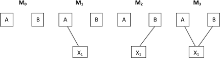
Figure 1: Interaction graphs for loglinear models with one covariate.

Example 1. Assume that there is one covariate $X_{1}$. The data are collated in a three-way contingency table $A\times B\times X_{1}$. The total population size estimates under loglinear models $M_{1}=[AX_{1}][B]$ and $M_{2}=[A][BX_{1}]$ are equal; this illustrates Property 2. Both total population size estimates are equal to the population size estimate under model $M_{0}=[A][B]$ in the two-way contingency table $A\times B$. Hence, the three-way table is collapsible over $X_{1}$ and this illustrates Property 1. In passing, we note that this result illustrates the second assumption of population size estimation from two registers discussed in the Introduction, namely, that the inclusion probabilities only need to be homogeneous for one of the two registers. The population size estimate under loglinear model $M_{3}=[AX_{1}][BX_{1}]$ is different from these population size estimates. See Figure 1 for interaction graphs of models $M_{0}$, $M_{1}$, $M_{2}$ and $M_{3}$.

We present a numerical example in Tables 2 and 3. Here $A$ refers to inclusion in the official register GBA, $B$ refers to inclusion in the police register HKS and the covariate $X_{1}$ is gender. See Section 2 for more details. We note that, even though the total population size estimates for models $M_{1}$ and $M_{2}$ are equal, estimates of the subpopulations (i.e., males and females) for $M_{1}$ are different from those under $M_{2}$.

=230pt Model Deviance df Missed $M_{0}$: $[A][B]$ 540.0 0 6170.3 $M_{1}$: $[AX_{1}][B]$ 548.5 1 6170.3 $M_{2}$: $[A][BX_{1}]$ 541.1 1 6170.3 $M_{3}$: $[AX_{1}][BX_{1}]$ 540.0 0 5696.1

Table 2: Models fitted to contingency table of variables $A$ (GBA), $B$ (HKS) and to $A,B$ and $X_{1}$ (gender), deviances, degrees of freedom and estimated numbers missed

= $\bm{A}$ $\bm{B}$ $\bm{X_{1}}$ obs $\bm{M_{1}}$ $\bm{M_{2}}$ $\bm{M_{3}}$ 1 1 1 972 629.2 976.5 972.0 2 1 1 234 234.0 229.5 234.0 1 2 1 14,883 15,225.8 14,883.0 14,883.0 2 2 1 0 5662.2 3497.9 3582.9 1 1 2 113 455.8 108.5 113.0 2 1 2 21 21.0 25.5 21.0 1 2 2 11,371 11,028.2 11,371.0 11,371.0 2 2 2 0 508.1 2672.5 2113.2

Table 3: Observed and fitted counts for the three-way table of $A$ (GBA), $B$ (HKS) and $X_{1}$ (gender); for $A$ and $B$ level 1 is present and for $X_{1}$ level 1 is male

Example 2. Suppose that there are two covariates, namely, $X_{1}$ and $X_{2}$. Table 4 presents a fairly comprehensive list of typical models including the estimated numbers missed and deviances. We note that models $M_{4}$, $M_{6}$ and $M_{6}^{\prime}$ have identical total population size estimates. Models $M_{5}$, $M_{8}$, $M_{9}$, $M_{11}$ and $M_{11}^{\prime}$ also have identical total population size estimates. The remaining models $M_{7}$, $M_{10}$ and $M_{12}$, $M_{12}^{\prime}$ and $M_{12}^{\prime\prime}$ have different total population size estimates.

= Model Deviance df Missed $M_{4}$ $[AX_{1}][BX_{2}]$ $617.6$ 13 6170.3 $M_{5}$ $[AX_{1}][BX_{1}][X_{2}]$ $228.6$ 15 5696.1 $M_{6}$ $[AX_{1}X_{2}][B]$ $718.2$ 7 6170.3 $M_{6}^{\prime}$ $[AX_{1}][AX_{2}][X_{1}X_{2}][B]$ $725.6$ 10 6170.3 $M_{7}$ $[AX_{1}][BX_{2}][X_{1}X_{2}]$ $588.6$ 10 6179.4 $M_{8}$ $[AX_{1}][BX_{1}][BX_{2}]$ $69.1$ 12 5696.1 $M_{9}$ $[AX_{1}][BX_{1}][X_{1}X_{2}]$ $200.2$ 12 5696.1 $M_{10}$ $[AX_{1}][BX_{2}][AX_{2}][BX_{1}]$ $65.9$ 9 5837.1 $M_{11}$ $[AX_{1}][BX_{1}X_{2}]$ $4.9$ 6 5696.1 $M_{11}^{\prime}$ $[AX_{1}][BX_{1}][BX_{2}][[X_{1}X_{2}]$ $34.4$ 9 5696.1 $M_{12}$ $[AX_{1}X_{2}][BX_{1}X_{2}]$ $0.0$ 0 5910.1 $M_{12}^{\prime}$ $[AX_{1}X_{2}][BX_{1}][BX_{2}]$ $23.3$ 3 6257.1 $M_{12}^{\prime\prime}$ $[AX_{1}][AX_{2}][BX_{1}][BX_{2}][X_{1}X_{2}]$ $31.2$ 6 5831.4

Table 4: Models fitted in four-way array of variables $A,B,X_{1}$ and $X_{2}$; registers $A$ (GBA), $B$ (HKS), covariates $X_{1}$ (gender), $X_{2}$ (age coded in four levels); deviances, degrees of freedom and estimated numbers missed

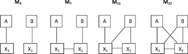
Figure 2: Interaction graphs of loglinear models with two covariates.

We discuss Properties 1 and 2 together. We use two notions from graph theory and graphical models, namely, of a path and a short path [e.g., see Whittaker (1990)]. The two registers $A$ and $B$ are connected by a path if there is a sequence of adjacent edges connecting the variables $A$ and $B$ in the graph. A short path from $A$ to $B$ is a path that does not contain a sub-path from $A$ to $B$. Figures 1 and 2 illustrate.

• In models where $A$ and $B$ are not connected, so that there is no path from $A$ to $B$, the contingency table can be collapsed over all of the covariates in the graph. So in Figure 1 the contingency table $A\times B\times X_{1}$ can be collapsed over $X_{1}$ in model $M_{1}$ and in model $M_{2}$. This illustrates Property 1 that under models $M_{1}$ and $M_{2}$ the population size estimate is identical to the population size estimate $M_{0}$. In this example this also implies Property 2, that models $M_{1}$ and $M_{2}$ have identical population sizes estimates. The table $A\times B\times X_{1}\times X_{2}$ can be collapsed over both $X_{1}$ and $X_{2}$ in models $M_{4}$, $M_{6}$ and $M_{6}^{\prime}$ because $X_{1}$ and $X_{2}$ are not on a short path from $A$ to $B$. In passing, we note this property of model $M_{4}$ shows that the inclusion probabilities of $A$ and of $B$ may both be heterogeneous as long as the sources of heterogeneity, that is, $X_{1}$ and $X_{2}$, are not related.

• In models with a short path connecting $A$ and $B$, the table is not collapsible over the covariates in the path. A simple example is model $M_{3}$ of Figure 1, where the contingency table $A\times B\times X_{1}$ cannot be collapsed over $X_{1}$. Another simple example is model $M_{7}$ of Figure 2, where the contingency table cannot be collapsed over either $X_{1}$ or $X_{2}$.

• When the covariate $X_{2}$ is not part of any path from $A$ to $B$ as in models $M_{5}$ and $M_{8}$, then $A\times B\times X_{1}\times X_{2}$ is collapsible over $X_{2}$, illustrating Property 1. Again, for this example, Property 1 implies Property 2, namely, that these models have identical population size estimates.

• For model $M_{11}$ of Figure 2 there are two paths from $A$ to $B$, $A-X_{1}-B$ and $A-X_{1}-X_{2}-B$; however, the table is collapsible over $X_{2}$, as the second path is not short, containing the unnecessary detour $X_{1}-X_{2}-B$.

• The other models have no covariates over which the contingency table can be collapsed. For example, in model $M_{12}$ of Figure 2, and its reduced versions $M_{12}^{\prime}$ and $M_{12}^{\prime\prime}$, there are again two short paths, one through $X_{1}$ and one path through $X_{2}$.

3.2 Two registers, covariates observed in only one of the registers

In Section 3.1 it is presumed that covariates are present in both register $A$ as well as in register $B$. Recently, it has been made possible to estimate the population size making use of covariates that are only observed in one of the registers [see Zwane and van der Heijden (2007); for examples, see van der Heijden, Zwane and Hessen (2009), and Sutherland, Schwartz and Rivest (2007)]. A simple example illustrates the problem [see Panel 1 of Table 5] where covariate $X_{1}$ (Marital status) is only observed in register $A$ (GBA) and covariate $X_{2}$ (Police region) is only observed in register $B$ (HKS). As a result, $X_{1}$ is missing for those observations not in $A$ and $X_{2}$ is missing for those observations not in $B$. Zwane and van der Heijden (2007) show that the missing observations can be estimated using the EM algorithm under a missing-at-random (MAR) assumption [Little and Rubin (1987), Schafer (1997a, 1997b)] for the missing data process. After EM, in a second step, the population size estimates are obtained for each of the levels of $X_{1}$ and $X_{2}$.

=295pt Panel 1: Observed counts $\bm{A=1}$ $\bm{A=2}$ $\bm{X_{1}=1}$ $\bm{X_{1}=2}$ $\bm{X_{1}}$ missing $B=1$ $X_{2}=1$ 259 539 13,898 $X_{2}=2$ 110 177 12,356 $B=2$ $X_{2}$ missing 091 164 – Panel 2: Fitted values under $[AX_{2}][BX_{1}][X_{1}X_{2}]$ $\bm{A=1}$ $\bm{A=2}$ $\bm{X_{1}=1}$ $\bm{X_{1}=2}$ $\bm{X_{1}=1}$ $\bm{X_{1}=2}$ $B=1$ $X_{2}=1$ 259.0 539.0 4510.8 9387.2 $X_{2}=2$ 110.0 177.0 4735.8 7620.3 $B=2$ $X_{2}=1$ 063.9 123.5 1112.4 2150.2 $X_{2}=2$ 027.1 040.5 1167.9 1745.4

Table 5: Covariate $X_{1}$ is only observed in register $A$ and $X_{2}$ is only observed in $B$

The number of observed cells is lower than in the standard situation. For example, in Panel 1 of Table 5 this number is $8$, whereas it would have been $12$ if both $X_{1}$ and $X_{2}$ were observed in both $A$ and $B$. For this reason only a restricted set of loglinear models can be fit to the observed data. Zwane and van der Heijden (2007) show that the most complicated model is $[AX_{2}][BX_{1}][X_{1}X_{2}]$; note that the graph is similar to the graph of $M_{7}$ in Figure 2, but $X_{1}$ and $X_{2}$ are interchanged. At first sight this model appears counter-intuitive, as one might expect an interaction between variables $A$ and $X_{1}$, and between $B$ and $X_{2}$. However, the parameter for the interaction between $A$ and $X_{1}$ (and $B$ and $X_{2}$) cannot be identified, as the levels of $X_{1}$ do not vary over individuals for which $A=2$.

This most complicated loglinear model $[AX_{2}][BX_{1}][X_{1}X_{2}]$ is saturated, as the number of parameters is $8$ (namely, the general mean, four main effect parameters and three interaction parameters) and there are just $8$ observed values. Consequently, these $8$ observed values are identical to the corresponding $8$ fitted values. The fitted values under this model are presented in Panel 2 of Table 5. Note that, for example, the EM algorithm spreads out the observed value 13,898 over the levels of $X_{1}$ into fitted values 4510.8 and 9387.2; note also that the ratio 4510.8/9387.2 of these fitted values is identical to the ratio 259/539 of the observed values.

By comparison, when $X_{1}$ and $X_{2}$ are observed in both $A$ and $B$, the saturated model is $M_{12}=[AX_{1}X_{2}][BX_{1}X_{2}]$. This is a less restrictive model than the model $[AX_{2}][BX_{1}][X_{1}X_{2}]$ and the difference is due to the MAR assumption.

We now consider the more general case when there are also covariates observed in both $A$ and $B$. Suppose that there is one covariate $X_{1}$ just observed in register $A$, one covariate $X_{2}$ just observed in register $B$, and one covariate $X_{3}$ observed in both registers. The most complicated model is $M_{13}=[AX_{2}X_{3}][BX_{1}X_{3}][X_{1}X_{2}X_{3}]$, with graph in Figure 3. When $X_{1}$ and $X_{2}$ are conditionally independent given $X_{3}$, the model simplifies to $M_{14}=[AX_{2}X_{3}][BX_{1}X_{3}]$. In $M_{14}$ there is only one short path, namely, $A-X_{3}-B$, and neither covariate $X_{1}$ and $X_{2}$ is part of it. Therefore, we can collapse the five-way table $A\times B\times X_{1}\times X_{2}\times X_{3}$ over $X_{1}$ and $X_{2}$, which illustrates Property 1. We conclude that inclusion of covariates that are unique to specific registers only modify the total population size estimate under the model $M_{13}$, in which the covariates just in $A$ are related to the covariates just in $B$.

Simplified situations exist when covariates $X_{1}$, $X_{2}$ or $X_{3}$ are not available. When $X_{1}$ is not available, $M_{13}$ reduces to model $[AX_{2}X_{3}][BX_{3}]$, where the table $A\times B\times X_{2}\times X_{3}$ is collapsible over $X_{2}$ because $X_{2}$ is not in the short path $A-X_{3}-B$. Hence, to improve the total population size estimate, covariates such as $X_{2}$ are not useful unless $X_{1}$ both exists and is related to $X_{2}$. Similarly, when $X_{2}$ is not available, $M_{13}$ reduces to $[AX_{3}][BX_{1}X_{3}]$ where the table is collapsible over $X_{1}$. When the covariate $X_{3}$ is not available, $M_{13}$ reduces to model $[AX_{2}][BX_{1}][X_{1}X_{2}]$, discussed earlier, where the covariates affect the population size when $X_{1}$ is related to $X_{2}$. If they are not related, the graph is similar to model $M_{4}$ and collapsing the contingency table over both $X_{1}$ and $X_{2}$ does not affect the total population size.

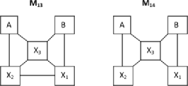
Figure 3: Interaction graphs of loglinear models with partially observed covariates.

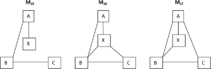
Figure 4: Interaction graphs of loglinear models with three registers and one covariate (see also next page).

3.3 Three registers

For completeness we give illustrative examples of the situation with three or more registers even though it is irrelevant for the data in Section 2, where there are only two. For three registers $A$, $B$ and $C$ the contingency table $A\times B\times{C}$ has one structural zero cell. We consider how the Properties apply to the context of three registers $A$, $B$ and $C$, and with a single covariate $X$. We discuss three models with their graphs displayed in Figure 4.

For model $M_{15}=[AX][AB][BC]$ the table $A\times B\times C\times X$ is collapsible over covariate $X$, as it is not on any short path. This illustrates Property 1. Property 2 is illustrated by the other models where $A$ and $C$ are conditionally independent given $B$ and $X$ is related to only one of the registers, namely, models $[AB][BC][BX]$ and $[AB][BC][CX]$.

For model $M_{16}=[ABX][BCX]$ covariate $X$ is on the short path from $A$ to $C$ and, therefore, the contingency table is not collapsible over $X$. For model $M_{17}=[ABX][BC][AC]$ covariate $X$ is not on the short path from $A$ to $B$, as the short path is $A-B$, and, therefore, the contingency table is collapsible over $X$.

The maximal model $[ABX][BCX][ACX]$ is discussed at the end of Appendix A.

4 Active and passive covariates

In Section 3 we discussed the result that marginalizing over a covariate does not necessarily lead to a change in the population size estimate. Whether the population size estimate changes or not depends on the loglinear models in the original and in the marginalized table. We term a covariate active if marginalizing over this covariate leads to a different estimate in the reduced table, so that this covariate plays an active role in determining the population size; we call a covariate passive if marginalizing leads to an identical estimate in the reduced table.

As an example we discuss active and passive covariates referring to Figure 3. We noted that in model $M_{13}$ the contingency table is not collapsible over covariates $X_{1}$ and $X_{2}$, hence, they are active covariates. On the other hand, in model $M_{14}$, by deleting the edge between $X_{1}$ and $X_{2}$, the contingency table is collapsible over $X_{1}$ and $X_{2}$, hence, they are passive covariates.

While passive covariates do not affect the size estimate, which suggests that they might be ignored, a possible use is the following. A secondary objective of population size estimation is to provide estimates of the size of subpopulations, or, equivalently, to break down the population size in terms of given covariates. This may well include passive covariates. Describing a population breakdown in terms of passive covariates is an elegant way to tackle this important practical problem. This extends the approach of Zwane and van der Heijden (2007) of using register specific covariates in the population size estimation problem.

Most registers have several covariates that are not common to other registers, because the different registers are set up with different purposes in mind. An interesting data analytic approach is, therefore, first, to determine a small number of active covariates, possibly of covariates that are in both registers; and second, to set up a loglinear model structured along the lines of model $M_{14}$, where several passive covariates can be entered by extending $X_{1}$ or $X_{2}$, and where these covariates may or may not be register specific. Passive covariates are helpful in breaking down the population size under the assumption that the passive covariates of register $A$ are independent of the passive covariates of register $B$ conditionally on the active covariates.

We note that the introduction of many covariates may lead to sparse contingency tables and hence to numerical problems due to empty marginal cells in those margins that are fitted. Consider, for example, a saturated model such as $[AX_{1}X_{2}X_{3}][BX_{1}X_{2}X_{3}]$. In this model the conditional odds ratios between $A$ and $B$ are 1. However, when a zero count in one of the subtables of $X_{1},X_{2}$ and $X_{3}$ occurs for the levels of $A$ and of $B$, the estimate in this subtable for the missing population is infinite. One way to solve this is by setting higher order interaction parameters equal to zero.

Another approach to tackle this numerical instability problem is as follows. We start with an analysis using only active covariates, for example, using the covariates observed in all registers in the saturated model. We may monitor the usefulness of the model by checking the size of the point estimate and its confidence interval. If the usefulness is problematic (e.g., when the upper bound of the parametric bootstrap confidence interval is infinite), we may make the model more stable by choosing a more restrictive model. One way to do this is by making a covariate passive. For example, both in model $[AX_{1}X_{2}][BX_{1}X_{2}X_{3}]$ as well as in model $[AX_{1}X_{2}X_{3}][BX_{1}X_{2}]$ the covariate $X_{3}$ is passive and both models yield identical estimates and confidence intervals. When one of these two model is chosen, its size may then be increased by adding additional passive variables, such as variables that are only observed in register $A$ or register $B$.

5 Example

We now discuss the analysis of the data introduced in Section 2. To recapitulate, $A$ is inclusion in the municipal register GBA and $B$ is inclusion in the police register HKS. Covariates observed in both $A$ and $B$ are $X_{1}$, gender, $X_{2}$, age (four levels), and $X_{3}$, nationality (1 $=$ Iraqi; 2 $=$ Afghan; 3 $=$ Iranian). Covariate $X_{4}$, marital status, is only observed in the municipal register GBA. Covariate $X_{5}$, police region where apprehended, with levels 1 $=$ in one of the four largest cities of the Netherlands, and 2 $=$ elsewhere, and is only observed in the police register HKS.

Table 6: Models fitted to example of variables $A,B,X_{1}$ to $X_{5}$, deviances, degrees of freedom, AIC’s, estimated population size and 95 percent confidence intervals

	Model	Deviance	df	AIC	Pop. size	CI
$N_{1}$	$[AX_{1}X_{2}X_{3}][BX_{1}X_{2}X_{3}]$	$0$	$0$	144.0	33,098.6	32,209–$\infty$468,
$N_{2}$	$[AX_{1}X_{2}][BX_{1}X_{2}X_{3}]$	$24.9$	$16$	136.8	33,504.1	32,480–35,468
$N_{3}$	$[AX_{1}X_{2}X_{3}][BX_{1}X_{2}]$	$28.8$	$16$	140.7	33,504.1	32,480–35,468
$N_{4}$	$[AX_{1}X_{2}X_{5}][BX_{1}X_{2}X_{3}X_{4}]$	$75.7$	$72$	315.7	33,504.1	32,480–35,468
$N_{5}$	$[AX_{1}X_{2}X_{5}][BX_{1}X_{2}X_{3}X_{4}][X_{4}X_{5}]$	$75.7$	$71$	317.7	33,503.8	32,395–35,543
$N_{6}$	$[AX_{1}X_{2}X_{3}X_{5}][BX_{1}X_{2}X_{4}]$	$523.8$	$72$	763.7	33,504.1	32,480–35,468
$N_{7}$	$[AX_{1}X_{2}X_{3}X_{5}][BX_{1}X_{2}X_{4}][X_{4}X_{5}]$	$289.1$	$71$	531.4	33,510.9	32,363–35,432

A first model is model $N_{1}=[AX_{1}X_{2}X_{3}][BX_{1}X_{2}X_{3}]$. This is a saturated model. For this model the estimate for the missed part of the population size is $5504.6$, and the total population size is $33\mbox{,}098.6$. However, the parametric bootstrap confidence interval [Buckland and Garthwire (1991)] shows that we deal with a solution that is numerically unstable, as the upper bound of the $95$ percent confidence interval is infinite. The instability of the model is a consequence of too many active covariates, and a solution is to make covariate $X_{3}$ passive. Two models in which $X_{3}$ is passive covariate are $N_{2}=[AX_{1}X_{2}][BX_{1}X_{2}X_{3}]$ and $N_{3}=[AX_{1}X_{2}X_{3}][BX_{1}X_{2}]$. For these models the population size estimate is $33\mbox{,}504.1$ ($95$ percent CI is $32\mbox{,}481$–$35\mbox{,}469$). Table 6 summarizes the results.

Models $N_{2}$ and $N_{3}$ are both candidates to be extended by including marital status ($X_{4}$) or police region ($X_{5}$). Note that $X_{4}$ is only observed in GBA ($A$) and $X_{5}$ is only observed in HKS ($B$). When $N_{2}$ is extended by adding $X_{4}$ and $X_{5}$ as passive variables, we get model $N_{4}[AX_{1}X_{2}X_{5}][BX_{1}X_{2}X_{3}X_{4}]$. This model yields an identical estimate for the missed part of the population, illustrating that in model $[AX_{1}X_{2}X_{3}X_{5}][BX_{1}X_{2}X_{3}X_{4}]$ the covariates $X_{4}$ and $X_{5}$ are indeed passive. With $72$ degrees of freedom and a deviance of $75.7$ the fit is good. The AIC is $315.7$. We check whether it is better to make covariates $X_{4}$ and $X_{5}$ active and we do this by adding the interaction between the covariates $X_{4}$ and $X_{5}$ to give model $N_{5}$. The deviance of this model is identical and we conclude that $N_{4}$ is a better working model than $N_{5}$. We also extend $N_{3}$ by adding $X_{4}$ and $X_{5}$ as passive variables giving $N_{6}$. Note again that the estimate for the missed part of the population is identical, however, the deviance is $523.8$ so the fit is worse. Adding the interaction between $X_{4}$ and $X_{5}$ in $N_{7}$ helps as the deviance goes to $289.1$, however, the deviance of $N_{7}$ is larger than the deviance of $N_{4}$, so we choose $N_{4}$ as the final model.

Out interest lies in the undocumented part of the population, that is, in the people not registered in the GBA. Table 7 shows the two-way margins of GBA with the other variables estimated under $N_{4}$. The estimates show that the undocumented population from Afghanistan, Iraq and Iran are mostly not included in the police register HKS, are more often male, between 25 and 50, from Afghanistan, unmarried and mostly not staying in the four largest cities.

Table 7: Estimates for GBA with each of the other variables under model $N_{4}$

	In HKS	Not in HKS	Male	Female
In GBA	1085.0	26,254.0	15,855.0	11,484.0
Not in GBA	0255.0	0,5910.0	0,3874.7	0,2290.3
	15–25	25–35	35–50	50–64
In GBA	7234.0	8361.0	9185.0	2559.0
Not in GBA	1292.2	2167.3	1925.9	0779.7
	Afghan	Iraqi	Iranian
In GBA	12,818.8	8743.3	5776.8
Not in GBA	0,2950.9	1914.5	1299.7
	Unmarried	Married	4 large cities	Elsewhere
In GBA	14,698.2	12,640.8	9720.0	17,619.0
Not in GBA	0,3302.3	0,2862.7	2182.6	0,3982.5

6 Conclusion

We have demonstrated two closely related properties of loglinear models in the context of population size estimation. First, under specific loglinear models marginalizing over covariates may leave the population size estimate unchanged. Second, different loglinear models fit to the same contingency table may yield identical population size estimates. This is worked out in detail for the case of two population registers and illustrated for the three-register case.

Using the first property, we have introduced the notion of active and passive covariates. In a specific loglinear model, marginalizing over an active covariate changes the population size estimate, while marginalizing over a passive variable leaves the population size estimate unchanged. This idea can be particularly powerful in those situations where each of the registers has unique covariates, but a description of the full population in terms of these covariates is needed. It may then be useful to introduce these register specific covariates as passive covariates into a model such as $M_{14}$. For example, if a loglinear model is proposed where the covariates unique to register $A$ are conditionally independent of the covariates unique to register $B$, then the full contingency tables is collapsible over these covariates and, hence, these covariates are passive.

Such a conditional independence assumption is strong, yet in many data sets there may not be enough power to test its correctness. It is demonstrated that a direct relation between the passive covariates of register $A$ and those in $B$ can only be assessed among those individuals that are in both register $A$ and $B$. If there is overlap between register $A$ and $B$, with relatively many individuals in both $A$ and $B$, the relationship between the passive covariates of $A$ and $B$ can easily be assessed; conversely, if the overlap is small, there is little power to establish whether or not this relation should be included in the model.

This new methodology should be of use for estimating the missing population due to undercoverage in the 2011 Census of the Netherlands where the size of the total population can be estimated by application of loglinear models. It could also be applied to countries that use register information to estimate the undercoverage of their Population Register as well as to countries which use traditional methods. The use of passive covariates gives insight into which characteristics individuals have that are not covered by the Census and thereby illuminate the bias due to the undercoverage.

In the Introduction we mentioned latent variable models that take heterogeneity of inclusion probabilities into account. For this purpose both Fienberg, Johnson and Junker (1999) as well as in Bartolucci and Forcina (2001) proposed generalizations of the so-called Rasch model. It is beyond the scope of this paper to study collapsibility properties for their models in the presence of covariates. However, it is interesting to note that one important specific form of the Rasch model, the so-called extended Rasch model, is mathematically equivalent to the loglinear model that includes three two-factor interactions that are identical and a three-factor interaction [see Hessen (2011); this loglinear model is also used in IWGDMF (1995), where it is referred to as a heterogeneity model]. Collapsibility properties of this loglinear model can be studied using the perspective presented in this paper.

Appendix A Identification of equivalent models

We establish which models listed in Figures 1–4 have the same estimates, and which do not, by showing that models for population size estimation are model collapsible onto two margins; and by demonstrating how the short path criterion identifies noninvariance of population size estimates. Our method is to apply the Asmussen and Edwards (1983) criterion to the population size estimation model which contains structural zeros.

A.1 Model collapsibility

First we recall the model collapsibility condition of Asmussen and Edwards (1983). Consider a table classified by two sets of factors $Y$ and $Z$, so that the saturated model is $[YZ]$, and maximum likelihood estimation under product multinomial sampling. The authors give conditions on the hierarchical loglinear model $M\subset[YZ]$ under which

$$\hat{p}^{N}_{Y}(y)=\sum_{z}\hat{p}^{M}_{YZ}(y,z),$$ (1)

where the right-hand side (RHS) is the margin of the MLE under the model $M$ for the full table, while the LHS is the MLE under the restricted model $N$ for the margin obtained by deleting terms in $Z$ from each generator of $M$. Their Theorem 2.3 states that $M$ is (model) collapsible onto the margin $Y$, that is, (1) holds, if and only if the boundary of every connected component of $Z$ is contained in a generator of $M$. A corollary to this result is that estimates computed under $N$ have the same sampling distribution as those under $M$, and hence the same confidence intervals.

Implicit in their derivation is that the space on which the table is defined is a Cartesian product of the factors. We argue that the population size estimation model cannot be defined on a Cartesian product of registers, for in our context if $p$ were defined on $\mathcal{A}\times\mathcal{B}\times\mathcal{X}$ with $\mathcal{A},\mathcal{B}=\{1,2\}$, then we require $p(2,2,x)=0$ to reflect a structural zero. If so, the maximal loglinear model would be $M=[ABX]$ with a three factor interaction, as $\log p$ contains the interaction term $\lambda_{ABX}(2,2,x)=-\infty$. Furthermore, application of model collapsibility suggests $M=[ABX]$ is model collapsible onto $[AB]$, which may be shown by counterexample to be false.

A.2 Models for population size estimation

For population size estimation the appropriate sample space $\mathcal{S}$ for two registers is

$$\mathcal{S}=\{(a,b);(a,b)=(1,1),(1,2),(2,1)\},$$

as $(2,2)$ cannot be observed, and the sample space for the whole survey is $\mathcal{S}\times\mathcal{X}$, where $\mathcal{X}$ is the Cartesian product of the discrete spaces for the covariates. Any loglinear model $M$ with probability mass function $p^{M}_{SX}$ is defined and fitted on this space. The loglinear expansion of $\log p^{M}_{SX}(a,b,x)$ under the maximal model $M=[AX][BX]$ is

$$\lambda+\lambda_{A}(a)+\lambda_{B}(b)+\lambda_{X}(x)+\lambda_{AX}(a,x)+\lambda_{BX}(b,x)$$ (2)

for $(a,b,x)\in\mathcal{S}\times\mathcal{X}$. The $\lambda$ parameters satisfy corner point constraints to ensure identifiability, but are otherwise arbitrary. This is an instance of a hierarchical loglinear model; an equivalent parameterization is to write the highest order main effect as $\lambda_{SX}(s,x)$, but this obscures the submodels of interest. The register $A$ taking values in $\mathcal{A}$ defines the marginal probability $p^{M}_{AX}$ of $p^{M}_{SX}$, similarly $p^{M}_{BX}$.

Asmussen and Edwards (1983) define the interaction graph to be the graph with a node for each factor classifying the table and an edge between two nodes if there is a generator in the model containing both. Consequently, the graphs in Figures 1–4 are the interaction graphs of particular population size models. The interaction graph of $M=[AX][BX]$ is that of $M_{3}$ in Figure 1 with $X$ replacing $X_{1}$.

These graphs cannot be interpreted as conditional independence graphs in which the missing edge between $A$ and $B$ leads to the statement $A\mathchoice{\mathrel{\hbox to0.0pt{$\displaystyle\perp$\hss}\mkern 4.1mu{\displaystyle\perp}}}{\mathrel{\hbox to0.0pt{$\textstyle\perp$\hss}\mkern 4.1mu{\textstyle\perp}}}{\mathrel{\hbox to0.0pt{$\scriptstyle\perp$\hss}\mkern 4.1mu{\scriptstyle\perp}}}{\mathrel{\hbox to0.0pt{$\scriptscriptstyle\perp$\hss}\mkern 4.1mu{\scriptscriptstyle\perp}}}B|X$, as this is false on the restricted space $\mathcal{S}\times\mathcal{X}$; for instance, if $X$ is empty, and $M=[A][B]$, then ${P}(A=1,B=1)\neq{p_{A}}(1){p_{B}}(1)$. However, conditional independence interpretations between a register and covariates, and between two covariates are possible.

With the population size estimation model at (2) defined on the right space, $\mathcal{S}\times\mathcal{X}$, we can now employ model collapsibility to show this model is collapsible onto two margins.

A.3 Model collapsibility for population size estimation

Our first result is that the maximal population size model in (2) is model collapsible onto its two margins $[AX]$ and $[BX]$. Standard arguments show the sufficient statistics are $n_{AX}(a,x)$ and $n_{BX}(b,x)$, where $n$ is the frequency function of the observations over the table. Under this model the MLEs satisfy $\hat{p}^{M}_{AX}=n_{AX}(a,x)/n_{\varnothing}$ and $\hat{p}^{M}_{BX}=n_{BX}(b,x)/n_{\varnothing}$; and these margins determine the full table $\hat{p}^{M}_{SX}$. To apply (1) when marginalizing over $B$, note the boundary of $\{A,B,X\}\setminus B$ in the interaction graph is $\{A,X\}$, and that these factors are both contained in a single generator of $M$, namely, $[AX]$. Similarly for marginalizing over $A$ so that the model is collapsible onto the two margins, and

$$\quad\hat{p}^{M}_{AX}(a,x)=\sum_{b}\hat{p}^{M}_{SX}(a,b,x),\qquad\hat{p}^{M}_{BX}(b,x)=\sum_{a}\hat{p}^{M}_{SX}(a,b,x).$$ (3)

A.4 Population size estimation invariance

We define population size estimation invariance, and show it depends on the model collapsibility of the population size model onto two margins, both containing one register and the covariates. Examples are given.

A population size estimate is made by extending the fitted probability $p^{M}_{SX}$ on $\mathcal{S}\times\mathcal{X}$ to $\pi^{M}$ defined on the Cartesian product space $\mathcal{A}\times\mathcal{B}\times\mathcal{X}$, by the conditional independence statement

$$\pi^{M}(a,b,x)=p^{M}_{AX}(a,x)p^{M}_{BX}(b,x)/p^{M}_{X}(x)\qquad\mbox{for }(a,b,x)\in\mathcal{A}\times\mathcal{B}\times\mathcal{X}.$$

Under the measure $\pi$ the interaction graphs in Figures 1–4 now have conditional independence interpretations.

The fitted values for $\hat{\pi}^{M}$ are computed from the fitted values $\hat{p}^{M}_{AX}$ and $\hat{p}^{M}_{BX}$ which are obtained from $\hat{p}^{M}(a,b,x)$ fitted on $\mathcal{S}^{2}\times\mathcal{X}$ at (3). The population size estimate is $n_{\varnothing}(1+\hat{\pi}^{M}(2,2))$, where

$$\hat{\pi}^{M}(a,b) = \sum_{x}\hat{p}^{M}_{AX}(a,x)\hat{p}^{M}_{BX}(b,x)/\hat{p}^{M}_{X}(x).$$ (4)

Two loglinear models $M$ and $N$ have identical population size estimates whenever $\hat{\pi}^{M}(a,b)=\hat{\pi}^{N}(a,b)$ for all $(a,b)\in\mathcal{A}\times\mathcal{B}$. So because of (4) the condition for invariance devolves to model collapsibility of ${M}$ on $\mathcal{A}\times\mathcal{X}$ and on $\mathcal{B}\times\mathcal{X}$.

We illustrate population size estimation invariance by showing that certain models for $\pi$ displayed in the figures above have identical estimates. The first example shows the model $M_{2}=[A][BX_{1}]$ in Figure 1 is collapsible on $X_{1}$ to $M_{0}=[A][B]$, and so produces identical population size estimates. From (4)

$$\hat{\pi}^{(2)}(a,b) = \sum_{x_{1}}\hat{p}^{(2)}_{A}(a)\hat{p}^{(2)}_{BX_{1}}(b,x_{1}),$$

by the independence of $A$ and $X_{1}$ under $M_{2}$. By the model collapsibility of $[BX_{1}]$ over $X_{1}$,

$$\hat{\pi}^{(2)}(a,b)=\hat{p}^{(2)}_{A}(a)\sum_{x_{1}}\hat{p}^{(2)}_{BX_{1}}(b,x_{1})=\hat{p}^{(0)}_{A}(a)\hat{p}^{(0)}_{B}(b),$$

which is just $\hat{\pi}^{(0)}(a,b)$ as required.

The second example is to show the model $M_{11}=[AX_{1}][BX_{1}X_{2}]$ in Figure 1 is collapsible on $X_{2}$ to $M_{3}=[AX_{1}][BX_{1}]$, and so produces identical population size estimates. From (4), using the independence $A$ and $X_{2}$ given $B,X_{1}$ under $M_{11}$,

$$\hat{\pi}^{(11)}(a,b) = \sum_{x_{1},x_{2}}\hat{p}^{(11)}_{AX_{1}}(a,x_{1})\hat{p}^{(11)}_{BX_{1}X_{2}}(b,x_{1},x_{2})/\hat{p}^{(11)}_{X_{1}}(x_{1}),$$

$$= \sum_{x_{1}}\hat{p}^{(11)}_{AX_{1}}(a,x_{1})/\hat{p}^{(11)}_{X_{1}}(x_{1})\sum_{x_{2}}\hat{p}^{(11)}_{BX_{1}X_{2}}(b,x_{1},x_{2})$$

$$= \sum_{x_{1}}\hat{p}^{(3)}_{AX_{1}}(a,x_{1})\hat{p}^{(3)}_{BX_{1}}(b,x_{1})/\hat{p}^{(3)}_{X_{1}}(x_{1}),$$

by the collapsibility of each of the three components in the expression and equals $\hat{\pi}^{(3)}(a,b)$ by definition.

A.5 Short path criterion for population size invariance

We demonstrate how the short path criterion identifies noninvariance in the context of an example attempting to argue that $M_{7}$ produces identical estimates to $M_{3}$.

First consider the population size estimate from $M_{7}$:

$$\hat{\pi}^{(7)}(a,b) = \sum_{x_{1},x_{2}}\hat{p}^{(7)}_{AX_{1}X_{2}}(a,x_{1},x_{2})\hat{p}^{(7)}_{BX_{1}X_{2}}(b,x_{1},x_{2})/\hat{p}^{(7)}_{X_{1}X_{2}}(x_{1},x_{2}).$$

Using the two independences under $M_{7}$,

$$\hat{\pi}^{(7)}(a,b) = \sum_{x_{1},x_{2}}\hat{p}^{(7)}_{AX_{1}}(a,x_{1})\hat{p}^{(7)}_{BX_{2}}(b,x_{2})\hat{p}^{(7)}_{X_{1}X_{2}}(x_{1},x_{2})/\hat{p}^{(7)}_{X_{1}}(x_{1})\hat{p}^{(7)}_{X_{2}}(x_{2})$$

$$= \sum_{x_{1}}\hat{p}^{(7)}_{AX_{1}}(a,x_{1})/\hat{p}^{(7)}_{X_{1}}(x_{1})\sum_{x_{2}}\hat{p}^{(7)}_{BX_{2}}(b,x_{2})\hat{p}^{(7)}_{X_{1}X_{2}}(x_{1},x_{2})/\hat{p}^{(7)}_{X_{2}}(x_{2}).$$

While model collapsibility implies $\hat{p}^{(7)}_{AX_{1}}(a,x_{1})=\hat{p}^{(3)}_{AX_{1}}(a,x_{1})$, simple counter examples show $\hat{p}^{(3)}_{BX_{1}}(b,x_{1})\neq\sum_{x_{2}}\hat{p}^{(7)}_{BX_{2}}(b,x_{2})\hat{p}^{(7)}_{X_{1}X_{2}}(x_{1},x_{2})/\hat{p}^{(7)}_{X_{2}}(x_{2})$. Here $X_{2}$ is on a short path from $A$ to $B$ and the population size estimates are not invariant to marginalizing over $X_{2}$.

The last model we consider is the maximal model for three registers $A$, $B$ and $C$ and covariate $X$, that is, $[ABX][ACX][BCX]$. It is collapsible over $A$, or $B$, or $C$, but it is not collapsible over $X$. Of course, population size estimates are not invariant to collapsing over $A$ even though $[ABX][ACX][BCX]$ is model collapsible over $A$, showing that population size invariance is not equivalent to model collapsibility.

Appendix B Estimation

Estimation of the missing count can be done as follows. We first discuss the case that there is no covariate. Let $A$ and $B$ have levels $a,b=1,2$, for “registered” and “not registered.” We denote observed frequencies by $n_{ab}$ with $(a,b)=(2,2)$ missing. Expected frequencies are denoted by $m_{ab}$ and fitted values by $\hat{m}_{ab}$. For the three cells $(a,b)$ with $(a,b)\neq(2,2)$ we define a loglinear independence model as log $m_{ab}=\lambda+\lambda_{A}(a)+\lambda_{B}(b)$ with $\lambda_{A}(2)=\lambda_{B}(b)=0$. Then, after fitting the loglinear model, the missing count $m_{22}$ is found as $\hat{m}_{22}=\exp(\hat{\lambda})$.

In the presence of a covariate $X$ with levels $x=1,2$, the observed counts are $n_{abx}$ with $(a,b,x)=(2,2,x)$ missing. A saturated loglinear model for the six observed counts is log $m_{abx}=\lambda+\lambda_{A}(a)+\lambda_{B}(b)+\lambda_{X}(b)+\lambda_{AX}(ax)+\lambda_{BX}(bx)$ with $\lambda_{A}(2)=\lambda_{B}(2)=\lambda_{X}(2)=0$. Then, after fitting a saturated or restricted loglinear model to the six observed counts, the missing counts are found as $\hat{m}_{221}=\exp(\hat{\lambda}+\hat{\lambda}_{X}(1))$ and $\hat{m}_{222}=\exp\hat{\lambda}$. This generalizes in a natural way to the situation that there are more registers, that covariates have more than two levels and more covariates.

Extra information is needed for the models in Section 3.2, where covariates are observed in only one of the registers. We follow the explanation in Zwane and van der Heijden (2007). The approach taken to analyze such data (data with partly available covariates) is to identify the problem as a missing information problem, and then use the EM algorithm to obtain maximum likelihood estimates.

The EM algorithm is an iterative procedure with two steps, namely, the expectation and maximization step. The EM algorithm starts with initial values for the probabilities to be estimated. Initial values have to be at the interior of the parameter space (i.e., not equal to zero), for example, form a uniform table, in which all the elements are equal. In the $t$th E-step, we compute the expected loglikelihood of the complete data conditional on the available data under the values of the parameters in that iteration. In the $t$th M-step, a loglinear model is fitted to the completed data, with the missing cells corresponding to $(a,b)=(2,2)$ denoted as structurally zero. The fitted probabilities under the loglinear model fitted in the M-step are then used in the E-step of the ($t+1$) iteration, to derive updates for the completed data.

Cycling between the E-step and the M-step goes on until convergence. At each iteration the likelihood increases. Convergence to a local maximum or a saddle point is guaranteed. Schafer [(1997a), pages 51–55] states that, in well-behaved problems (i.e., problems with not too many missing entries and not too many parameters), the likelihood function will be unimodal and concave on the entire parameter space, in which case EM converges to the unique maximum likelihood estimate from any starting value. Thus far, we have never encountered examples where multiple maxima exist, and a typical way to investigate the presence of multiple maxima is by trying out different starting values.

After convergence, the fit is assessed using the observed elements only (e.g., for Table 5 there are only 8 observed elements, whereas in the completed table, excluding the structural zero cells, there are 12 elements). Degrees of freedom are determined using the number of observed elements minus the number of fitted parameters.

The values for the missing cells corresponding to $(a,b)=(2,2)$ are assessed using the method that we described above.

We use parametric bootstrap confidence intervals because they provide a simple way to find the confidence intervals when the contingency table is not fully observed. To compute the bootstrapped confidence intervals for a specific loglinear model, we need to first compute the population size under this model and the probabilities on the completed data under this model, that is, by including the cells that cannot be observed by design. A first multinomial sample is drawn given these parameters, and the sample is then reformatted to be identical to the observed data. The specific loglinear model used is then fitted to the resulting data, resulting in the first bootstrap sample estimate of the population size. If $K$ bootstrap samples are needed, then this is repeated $K$ times. By ordering the $K$ bootstrap population size estimates, a confidence interval can be constructed.

Estimation in R [doi]10.1214/12-AOAS536SUPP [url]http://lib.stat.cmu.edu/aoas/536/supplement.pdf .pdf We make use of the CAT-procedure in R (Meng and Rubin (1991); Schafer [(1997a), Chapters 7 and 8], (1997b)). The CAT-procedure is a routine for the analysis of categorical variable data sets with missing values. We describe our application of this procedure in detail in the supplemental article [van der Heijden et al. (2012)].