An all-purpose metric for the exterior of any kind of rotating neutron star

Abstract

We have tested the appropriateness of two-soliton analytic metric to describe the exterior of all types of neutron stars, no matter what their equation of state or rotation rate is. The particular analytic solution of the vaccuum Einstein equations proved quite adjustable to mimic the metric functions of all numerically constructed neutron-star models that we used as a testbed. The neutron-star models covered a wide range of stiffness, with regard to the equation of state of their interior, and all rotation rates up to the maximum possible rotation rate allowed for each such star. Apart of the metric functions themselves, we have compared the radius of the innermost stable circular orbit $R_{\rm{ISCO}}$, the orbital frequency $\Omega\equiv\frac{d\phi}{dt}$ of circular geodesics, and their epicyclic frequencies $\Omega_{\rho},\Omega_{z}$, as well as the change of the energy of circular orbits per logarithmic change of orbital frequency $\Delta\tilde{E}$. All these quantities, calculated by means of the two-soliton analytic metric, fitted with good accuracy the corresponding numerical ones as in previous analogous comparisons (although previous attempts were restricted to neutron star models with either high or low rotation rates). We believe that this particular analytic solution could be considered as an analytic faithful representation of the gravitation field of any rotating neutron star with such accuracy, that one could explore the interior structure of a neutron star by using this space-time to interpret observations of astrophysical processes that take place around it.

1 Introduction

The amount and accuracy of modern observations in various parts of the electromagnetic spectrum has increased dramatically. In order to give astrophysically plausible explanations of the various problems related to the observations we have to rely on theoretical assumptions that are at least as accurate as the data we are trying to analyze. There is a large class of observations (see e.g., van der Klis (2006)) that are related to the astrophysical environment of compact relativistic objects (AGNs, LMXBs, etc). Furthermore, the anticipated successful gravitational wave detection will open a new window to observe such objects. In order to understand these phenomena, one has to have a sufficiently accurate analytic description of the spacetime around such compact objects. If the central object is a black hole, there is a unique choice in the framework of general relativity: the Kerr spacetime. On the other hand the geometry around a rotating neutron star is much more complicated, since it depends on many parameters related to the internal structure of the neutron star and the way it rotates.

The assumption that the geometry around such an object is approximately that of a Schwarzschild, or a Kerr metric (see for example van der Klis (2006)) is very simplistic and it may lead to erroneous conclusions about the actual astrophysical processes that take place in the close neighborhood of the star itself (cf. Pappas (2012); Pachón, Rueda & Valenzuela-Toledo (2012)).

One can alternatively rely on numerical codes that are able to describe the geometry around a realistic neutron star in a tabular form on a given grid with sufficiently high accuracy. There are various groups (see Stergioulas & Friedman (1995), and for an extended list of numerical schemes see Stergioulas (2003)), that have acquired expertise in building relativistic models of astrophysical objects with adjustable physical characteristics and constructing the metric inside and outside such objects by solving numerically the full Einstein equations in stationary, axisymmetric cases.

Although studying astrophysical phenomena in a geometric background that has been constructed numerically is plausible, there are certain drawbacks in using such metrics: (i) Computing various physical quantities of a system, like the orbital frequencies, or the innermost circular orbit, from a metric that is given in a tabular form is not very practical and is often plagued by numerical errors. (ii) Astrophysical observations from the environment of a compact object could be used to read the physical parameters that are related to the structure of the compact object such as its mass, its equation of state, its rotation, or to obtain the law of its differential rotation, etc. This would be very difficult to achieve with a metric that is numerically constructed. Solving the inverse problem by means of a numerical metric is a blind process that can not be easily led by physical insight. Instead an analytic expression for the corresponding spacetime would be much more preferable.

There are various analytic metrics that have been used in the past to describe the exterior geometry of a neutron star. As mentioned above, the Schwarzschild metric is not accurate enough for rotating neutron stars, while the Kerr metric is good only for a collapsed object (a black hole) but it fails to describe the exterior of a neutron star, as comparisons of Kerr with numerical geometries of rotating neutron stars by Berti & Stergioulas (2004) have shown.

The Hartle-Thorne metric of Hartle & Thorne (1968), which has been constructed as an approximate solution of the vacuum Einstein equations (VEE) for the exterior of a slowly rotating star, has been extensively used by various authors to describe neutron stars of low rotation rate (see for example Berti et al. (2004)). Finally, various other analytic solutions of VEE have been constructed and some of them have been used, especially during the last decade, to describe the exterior geometries of neutron stars (see Stute & Camenzind (2002); Berti & Stergioulas (2004); Pachón, Rueda & Sanabria-Gómez (2006); Pappas (2009); Teichmüller, Fröb & Maucher (2011)). Such solutions are based on the formalism developed by Ernst (1968a, b) which reformulates Einstein equations in the case of axisymmetric, stationary space-times. Manko et al. and Sibgatullin (see the articles of Sibgatulin (1984); Manko & Sibgatulin (1993); Manko, Martin & Ruiz (1995); Ruiz, Manko & Martin (1995); Manko, Mielke & Sanabria-Gómez (2000)) have used various analytic methods to produce such space-times parameterized by various parameters that have different physical context depending on the type of each solution.

Such an analytic solution, with its parameters appropriately adjusted to match numerical models of neutron stars, could then be used to describe the stationary properties of the space-time around the neutron star itself; that is, study the geodesics in the exterior of the neutron star. More specifically, from the analytic solution we could obtain bounds of motion for test particles orbiting the neutron star, find the location of the innermost stable circular orbit (ISCO), compute the orbital frequency of the circular orbits on the equatorial plane as well as the epicyclic frequencies around it and perform any sort of dynamical analysis on the geodesics (for example see Lukes-Gerakopoulos (2012)). These properties of the space-time could be used to study quantitatively astrophysical phenomena that take place in the vicinity of neutron stars, such as accretion discs. Inversely one could use the astrophysical observations related to such phenomena to determine the parameters describing the analytic space-time and from that acquire information for the central object.

The central issue with analytic metrics is whether one can find solutions that are able to describe with sufficient faithfulness all kinds of rotating neutron stars; either slowly or rapidly rotating ones, or even differentially rotating ones.

One solution that has been recently used by Stute & Camenzind (2002) and later by Berti & Stergioulas (2004) to describe the exterior space-time of rotating neutron stars is the three-parameter solution of Manko, Mielke & Sanabria-Gómez (2000) (also mentioned as Manko et al.). Although this solution was shown to match quite well the space-time of highly rotating neutron stars, it failed to match the slowly rotating ones. The reason for failing to describe slow rotation is that in the zero angular momentum limit, this particular solution has a non vanishing quadrupole moment, while one would expect slowly rotating neutron stars to be approximately spherically symmetric. This problem of the Manko et al. solution was not considered disappointing by Berti and Stergioulas, since the space-time around slowly rotating stars could be described equally well by the Hartle-Thorne approximation.

The three-parameter solution of Manko et al. is a special case of the so called two-soliton solution, which was constructed by Manko, Martin & Ruiz (1995). The two-soliton is a four-parameter analytic metric which, contrary to the previous one, can be continuously reduced to a Scwarzschild or a Kerr metric while it does not suffer from the problematic constraints of the Manko et al. solution with respect to the anomalous behavior of its quadrupole moment. Actually the first four multiple moments of the two-soliton solution can be freely chosen. Of course the analytic form of the two-soliton solution is not as compact as the Manko et al. solution, but this is the price one has to pay in order to cover the whole range of the physical parameters of a neutron star with a single analytic metric.

In the present work, that constitutes the extension and completion of preliminary results presented by Pappas (2009), that were suitably corrected with respect to the right extraction of the multipole moments of the numerical space-time as was recently demonstrated by Pappas & Apostolatos (2012), we are using this two-soliton solution to describe the space-time around a wide range of numerically constructed rotating neutron stars. We use the numerical multipole moments to set the multipole moments of the analytic space-time. Then we examine how well the two metrics match each other. Moreover we have performed comparisons between astrophysicaly relevant geometric quantities produced from the numerical and the analytic space-times, like the position of the innermost stable circular orbit (ISCO), the orbital frequencies, the epicyclic frequencies that are related to slightly non-circular and slightly non-equatorial orbits, and the change of energy of the circular orbits per logarithmic change of the orbital frequency, $\Delta\tilde{E}$. The overall picture is that the new metric matches the numerical one with excellent accuracy for all rotation rates and all equations of state.

The rest of the paper is organized as follows: In Sec. 2 the proposed analytic solution (two-soliton) is briefly presented and some of its properties are thoroughly analyzed. The parameter space of the two-soliton is investigated and it is shown how to obtain the limiting cases of Schwarzschild, Kerr and Manko et al. A brief discussion of the physical properties of the space-time such as the presence of singularities, horizons, ergoregions and regions of closed timelike curves (CTCs) is also given. In Sec. 3 we show how we match the analytic two-soliton solution to a specific numerical one by matching the first four multipole moments, and show why this is generally the best choice. In Sec. 4 we discuss various criteria that could be used to compare the two metrics. Finally, in Sec. 5 the final comparison criteria and the results of the corresponding comparisons are presented. In Sec. 6 we give an overview of the conclusions obtained by our study.

2 The two-soliton solution

The vacuum region of a stationary and axially symmetric space-time can be described by the Papapetrou line element, which was first used by Papapetrou (1953),

$$ds^{2}=-f\left(dt-\omega d\phi\right)^{2}+f^{-1}\left[e^{2\gamma}\left(d\rho^{2}+dz^{2}\right)+\rho^{2}d\phi^{2}\right],$$ (1)

where $f,\;\omega,$ and $\gamma$ are functions of the Weyl-Papapetrou coordinates ($\rho,z$). By introducing the complex potential $\mathcal{E}(\rho,z)=f(\rho,z)+\imath\psi(\rho,z)$, Ernst (1968a) reformulated the Einstein field equations for this type of space-times in a concise complex equation

$$(Re(\mathcal{E}))\nabla^{2}\mathcal{E}=\nabla\mathcal{E}\cdot\nabla\mathcal{E}.$$ (2)

The real part of the Ernst potential $\mathcal{E}$ is the metric function $f$, which is also the norm of the timelike Killing vector related with stationarity, while $\psi$ is a scalar potential related with the twist of the same vector.

A general procedure for generating solutions of the Ernst equations was developed by Sibgatulin (1984); Manko & Sibgatulin (1993); Ruiz, Manko & Martin (1995); Manko, Martin & Ruiz (1995). Each solution of the Ernst equation is produced from a choice of the Ernst potential along the axis of symmetry of the metric in the form of a rational function

$$\mathcal{E}(\rho=0,z)=e(z)=\frac{P(z)}{R(z)},$$ (3)

where $P(z),R(z)$ are polynomials of $z$ of order $n$ with complex coefficients in general. The algorithm developed by Ruiz, Manko & Martin (1995) works as follows: First the Ernst potential along the axis is expressed in the form

$$e(z)=1+\sum^{n}_{k=1}\frac{e_{k}}{z-\beta_{k}},$$ (4)

where $\beta_{k}$ are the roots of the polynomial $R(z)$ and $e_{k}$ are complex coefficients appropriately chosen so that the latter form of $e(z)$ (eq. 4) is equal to the former one (eq. 3). Subsequently one determines the $2n$ roots of equation

$$e(z)+e^{*}(z)=0,$$ (5)

where ^∗ denotes complex conjugation. These roots are denoted as $\xi_{k}$, with $k=1,2,\ldots,2n$ and from these one defines the $2n$ complex functions $R_{k}=\sqrt{\rho^{2}+(z-\xi_{k})^{2}}$. All these functions and roots are then used as building blocks for the following determinants

$$E_{\pm}=\left|\begin{array}[]{cccc}1&1&\cdots&1\\ \pm 1&&&\\ \vdots&&&\\ \pm 1&&&\\ &&\bf{C}&\\ 0&&&\\ \vdots&&&\\ 0&&&\\ \end{array}\right|\\$$ (6)

$$G=\left|\begin{array}[]{cccc}0&R_{1}+\xi_{1}-z&\cdots&R_{2n}+\xi_{2n}-z\\ -1&&&\\ \vdots&&&\\ -1&&&\\ &&\bf{C}&\\ 0&&&\\ \vdots&&&\\ 0&&&\end{array}\right|$$ (7)

$$H=\left|\begin{array}[]{cccc}z&1&\cdots&1\\ -\beta_{1}&&&\\ \vdots&&&\\ -\beta_{n}&&&\\ &&\bf{C}&\\ e^{*}_{1}&&&\\ \vdots&&&\\ e^{*}_{n}&&&\end{array}\right|$$ (8)

$$K_{0}=\left|{{\begin{array}[]{ccc}{\frac{1}{\xi_{1}-\beta_{1}}}&\cdots&{\frac{1}{\xi_{2n}-\beta_{1}}}\\ \vdots&\ddots&\vdots\\ {\frac{1}{\xi_{1}-\beta_{n}}}&\cdots&{\frac{1}{\xi_{2n}-\beta_{n}}}\\ {\frac{e^{*}_{1}}{\xi_{1}-\beta_{1}^{\ast}}}&\cdots&{\frac{e^{*}_{1}}{\xi_{2n}-\beta_{1}^{\ast}}}\\ \vdots&\ddots&\vdots\\ {\frac{e^{*}_{n}}{\xi_{1}-\beta_{n}^{\ast}}}&\cdots&{\frac{e^{*}_{n}}{\xi_{2n}-\beta_{n}^{\ast}}}\\ \end{array}}}\right|$$ (9)

where $\bf{C}$ is the $2n\times 2n$ matrix

$$\bf{C}=\left({{\begin{array}[]{ccc}{\frac{R_{1}}{\xi_{1}-\beta_{1}}}&\cdots&{\frac{R_{2n}}{\xi_{2n}-\beta_{1}}}\\ \vdots&\ddots&\vdots\\ {\frac{R_{1}}{\xi_{1}-\beta_{n}}}&\cdots&{\frac{R_{2n}}{\xi_{2n}-\beta_{n}}}\\ {\frac{e^{*}_{1}}{\xi_{1}-\beta_{1}^{\ast}}}&\cdots&{\frac{e^{*}_{1}}{\xi_{2n}-\beta_{1}^{\ast}}}\\ \vdots&\ddots&\vdots\\ {\frac{e^{*}_{n}}{\xi_{1}-\beta_{n}^{\ast}}}&\cdots&{\frac{e^{*}_{n}}{\xi_{2n}-\beta_{n}^{\ast}}}\\ \end{array}}}\right).$$ (10)

The Ernst potential and the metric functions are finally expressed in terms of the determinants given above as:

$${\mathcal{E}}(\rho,z) = \frac{E_{+}}{E_{-}},$$ (11)

$$f(\rho,z) = \frac{E_{+}E_{-}^{\ast}+E_{+}^{\ast}E_{-}}{2E_{-}E_{-}^{\ast}},$$ (12)

$$e^{2\gamma(\rho,z)} = \frac{E_{+}E_{-}^{\ast}+E_{+}^{\ast}E_{-}}{2K_{0}K_{0}^{\ast}\prod\nolimits_{k=1}^{2n}{R_{k}}},$$ (13)

$$\omega(\rho,z) = \frac{2\;\Im\left[{E_{-}H^{\ast}-E_{-}^{\ast}G}\right]}{E_{+}E_{-}^{\ast}+E_{+}^{\ast}E_{-}}.$$ (14)

We should note that due to the form of the metric functions, the parameters $e_{k}$ and their complex conjugates $e^{*}_{k}$ that appear in the determinants cancel out (the $\prod_{k=1}^{n}e_{k}e^{*}_{k}$ is a common factor of all products of determinants that show up in the metric functions), so they do not affect the final expressions.

The vacuum two-soliton solution (proposed by Manko, Martin & Ruiz (1995)) is a special case of the previous general axisymmetric solution that is obtained from the ansatz (see also Sotiriou & Pappas (2005))

$$e(z)=\frac{(z-M-ia)(z+ib)-k}{(z+M-ia)(z+ib)-k},$$ (15)

where all the parameters $M,a,k,b$ are real. From the Ernst potential along the axis one can compute the mass and mass-current moments of this space-time. Particularly, for the two-soliton space-time the first five non-vanishing moments are:

$$M_{0} = M,\quad M_{2}=-(a^{2}-k)M,$$

$$M_{4} = \left[a^{4}-(3a^{2}-2ab+b^{2})k+k^{2}-\frac{1}{7}kM^{2}\right]M$$

$$J_{1} = aM,\quad J_{3}=-[a^{3}-(2a-b)k]M.$$ (16)

The mass moments of odd order and the mass-current moments of even order are zero due to reflection symmetry with respect to the equatorial plane $(z=0)$ of the space-time (this is actually ensured by restricting all parameters of eq. (15) to assume real values). From the moments we see that the parameter $M$ corresponds to the mass monopole of the space-time, the parameter $a$ is the reduced angular momentum, $k$ is the deviation of the reduced quadrupole from the corresponding Kerr quadrupole (the one that has the same $M$ and $a$), and $b$ is associated with the deviation of the current octupole moment from the current octupole of the corresponding Kerr.

Table 1: Classification of the various two-soliton solutions depending on the values of the parameters $d,~{}\kappa_{\pm},~{}\xi_{\pm},~{}R_{\pm}$ and $r_{\pm}$. The table also shows the various conjugation relations between the parameters. The types of solutions that have degeneracies are indicated with an asterisk (^∗). $\Re$ means real, $\Im$ means imaginary, and ${\mathbf{C}}$ means complex.

Case	$d^{2}$	$\kappa_{+}^{2}$	$\kappa_{-}^{2}$	$\xi_{+}$	$\xi_{-}$	$R_{+}$	$R_{-}$	$r_{+}$	$r_{-}$
$Ia$	$>0$	$>0$	$>0$	$\Re$	$\Re$	$\Re$	$\Re$	$\Re$	$\Re$
$Ib^{*}$	$>0$	$>0$	$=0$	$\Re$	$\Re$	$\Re$	$\Re$	$\Re$	$\Re$
					$=\xi_{+}$			$=R_{+}$	$=R_{-}$
$IIa$	$>0$	$>0$	$<0$	$\mathbf{C}$	$\mathbf{C}$	$\mathbf{C}$	$\mathbf{C}$	$\mathbf{C}$	$\mathbf{C}$
					$=(\xi_{+})^{*}$			$=(R_{+})^{*}$	$=(R_{-})^{*}$
$IIb^{*}$	$>0$	$=0$	$<0$	$\Im$	$\Im$	$\mathbf{C}$	$\mathbf{C}$	$\mathbf{C}$	$\mathbf{C}$
					$=(\xi_{+})^{*}$		$=(R_{+})^{*}$	$=R_{-}$	$=R_{+}$
$IIc$	$>0$	$<0$	$<0$	$\Im$	$\Im$	$\mathbf{C}$	$\mathbf{C}$	$\mathbf{C}$	$\mathbf{C}$
							$=(R_{+})^{*}$		$=(r_{+})^{*}$
$III$	$<0$	$\mathbf{C}$	$\mathbf{C}$	$\Re$	$\Im$	$\Re$	$\Re$	$\mathbf{C}$	$\mathbf{C}$
			$=(\kappa_{+}^{2})^{*}$						$=(r_{+})^{*}$
$IVa^{*}$	$=0$	$>0$	$=\kappa_{+}^{2}$	$\Re$	$=0$	$\Re$	$\Re$	$\Re$	$\Re$
				$=\kappa_{+}$					$=r_{+}$
$IVb^{*}$	$=0$	$=0$	$=0$	$=0$	$=0$		-	-	-
$IVc^{*}$	$=0$	$<0$	$=\kappa_{+}^{2}$	$\Im$	$=0$	$\mathbf{C}$	$\mathbf{C}$	$\Re$	$\Re$
				$=\kappa_{+}$					$=r_{+}$

For the two-soliton ansatz (15), the characteristic equation (5) takes the form,

$$z^{4}-(M^{2}-a^{2}-b^{2}+2k)z^{2}+(k-ab)^{2}-b^{2}M^{2}=0.$$ (17)

Since the coefficients of the polynomial are real, the roots can be either real, or conjugate pairs. The four roots of (17) can be written as,

$$\xi_{1}=-\xi_{3}=\xi_{+},\;\;\xi_{2}=-\xi_{4}=\xi_{-},$$ (18)

where,

$$\xi_{\pm}=\frac{1}{2}\left(\kappa_{+}\pm\kappa_{-}\right),$$ (19)

with

$$\kappa_{\pm}=\sqrt{M^{2}-a^{2}-b^{2}+2k\pm 2d},$$ (20)

and

$$d=\sqrt{(k-ab)^{2}-b^{2}M^{2}}.$$ (21)

Using these symbols for the four roots we redefine the four corresponding functions $R_{k}$ as

$$R_{\pm}=\sqrt{\rho^{2}+(z\pm\xi_{+})^{2}},\;r_{\pm}=\sqrt{\rho^{2}+(z\pm\xi_{-})^{2}}.$$ (22)

Next we proceed to classify the various types of solutions depending on whether the four roots have real, purely imaginary or complex values. This classification is outlined in Table 1.

1. This case is characterized by two real roots $\xi_{\pm}$. The Kerr family of solutions, which corresponds to $k=0$ is definitely not included in this family of solutions.

   1. This subfamily of case I is the simplest to compute, since all functions $R_{\pm},r_{\pm}$ are real.

   2. This is a degenerate case where the roots $\xi_{\pm}$ coincide. The degeneracy is due to $\kappa_{-}$ being zero which corresponds to the parameter constraint $M^{2}-a^{2}-b^{2}+2k-2d=0$. In such degenerate cases, the computation of the metric function is not straightforward since the expressions for the metric become indeterminate, and a limiting procedure should then be applied. In the reduced-parameter space $({a}/{M},{b}/{M},{k}/{M^{2}})$, the previous constraint corresponds to a two-dimensional surface.

2. In this case, the roots $\xi_{\pm}$ are either complex or imaginary, since $\kappa_{-}^{2}<0$. Furthermore this means that there are nonvanishing values of $(\rho,z)$ where the functions $R_{\pm},r_{\pm}$ assume zero value, which then leads to singularities at the corresponding points.

   1. This sub-case, as with Case I, belongs to a class of solutions that cannot have a vanishing parameter $k$.

   2. Here, a degeneracy shows up again as in Case Ib, which admits the same treatment (limiting procedure) as in the former situation. Contrary to all previous cases, Case IIb admits a Kerr solution that belongs to the hyper-extreme branch ($|a|>M$). Similarly to Case Ib this solution is also represented by a two dimensional surface in the reduced-parameter space.

   3. This case is similar to the previous one, without the degeneracy in the roots $\xi_{\pm}$. It also includes hyper-extreme Kerr solutions.

3. In this case one of the $\xi_{+},\xi_{-}$ is real while the other one is imaginary. Thus the same type of singularity issues, as in Case II arise. In particular such problematic behavior shows up on the $z=0$ plane. The Kerr and the Schwarzschild solutions lie entirely within this family of solutions.

4. All types of solutions belonging to this case are degenerate (there is a special constraint between the parameters) and as such are probably of no interest to realistic neutron stars. Subcases IVa and IVc have one double root ($\xi_{-}=0$), while subcase IVb has a quadruple root ($\xi_{+}=\xi_{-}=0$) and the computation of the metric functions needs special treatment. We should also note that cases IVb and IVc include the extreme Kerr solution ($|a|=M$) as a special case.

As we can see from the classification, the two-soliton solution can produce a very rich family of analytic solutions with the classical solutions of Schwarzschild and Kerr being special cases of the general solution. Also the Manko et al. solution of Manko, Mielke & Sanabria-Gómez (2000) that has been used previously by Berti & Stergioulas (2004); Stute & Camenzind (2002) to match the exterior space-time of rotating neutron stars is a special case of the two-soliton solution as we will see next.

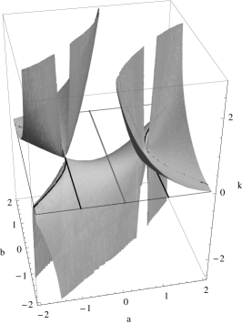
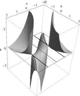
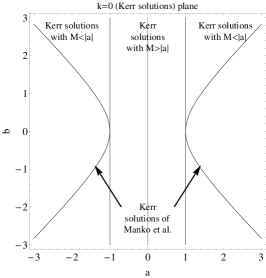
Figure 1: The first two plots show the parameter space $(a,b,k)$ of the two soliton solution for a particular mass ($M=1$) from two different view points so that the intricate foldings of the surface are better understood. The 2D surface plotted is the constraint of $k$ which corresponds to the solution of Manko et al. used by Berti & Stergioulas (2004). The third plot is the $k=0$ plane of the parameter space which corresponds to all Kerr solutions. The plots clearly show that the Manko et al. solution has no set of parameters to describe the case $k=0$ which corresponds to the Kerr and the Schwarzschild (for $a=0$) solutions, since there is no intersection of the constraint of $k$ and the Kerr plane in the appropriate range of parameters. The two hyperbolas plotted on the plane $k=0$ are the only points were the constraint of $k$ touches the plane tangentially. As we can see these hyperbolas correspond to $|a|>M$, i.e., to hyper-extreme Kerr space-times.

All types of solutions discussed above can be represented in a three dimensional parameter space, the reduced-parameter space that was mentioned in Case IIb. Although the two-soliton solution is characterized by four parameters, one of them, the monopole mass $M$, is simply a scaling parameter which can be used to reduce the rest of the parameters to dimensionless ones. The three dimensionless parameters thus formed, $({a}/{M},{b}/{M},{k}/{M^{2}})$, are related to the multipole moments (see eq. (2)) of the corresponding space-time in the following way: The first parameter ${a}/{M}$ is the spin parameter (where $a$ is the reduced angular momentum) which is the only parameter, besides the mass, that uniquely characterizes a Kerr space-time. The second parameter ${k}/{M^{2}}$ expresses the deviation of the quadrupole moment of the solution from the quadrupole moment of the corresponding Kerr (the one with the same ${a}/{M}$ value); an increase of the value of ${k}/{M^{2}}$ produces solutions that are less oblate than Kerr. The final parameter ${b}/{M}$ controls in a linear fashion the current octupole moment. The actual deviation of the two soliton octupole moment from the Kerr octupole moment depends on all three parameters ${a}/{M}$, ${k}/{M^{2}}$ and ${b}/{M}$. Of course the higher moments are also affected by these parameters.

In this three dimensional parameter space, the plane $k/M^{2}=0$ corresponds to all types of Kerr solutions. This is clear from the form of the Ernst potential along the axis, where if one sets $k=0$ it reduces to the Ernst potential of the Kerr solution,

$$e(z)=\frac{z-M-ia}{z+M-ia}.$$ (23)

Obviously in this case the parameter $b/M$ is redundant; thus each line ${a}/{M}=\textrm{const}$, which is parallel to the ${b}/{M}$ axis on the plane ${k}/{M^{2}}=0$, corresponds to a single Kerr (modulo the mass of the black hole).

As mentioned in the introduction, the solution of Manko, Mielke & Sanabria-Gómez (2000) has been used to describe the exterior of rotating neutron stars. As it was briefly discussed above this solution is included in the two-soliton solution and can be obtained by imposing a specific constraint on the two-soliton parameters. The Manko et al. solution is obtained by setting

$$k=-\frac{1}{4}\left[M^{2}-(a-b)^{2}\right]-\frac{M^{2}b^{2}}{M^{2}-(a-b)^{2}}+ab.$$ (24)

This constraint defines a surface in the three parameter space $({a}/{M},{b}/{M},{k}/{M^{2}})$ (see Figure 1). The particular solution, depending on the values of $a,b$, falls under either Case Ib or Case IIb, where either $\kappa_{-}$ or $\kappa_{+}$ is equal to zero, respectively. We should note that the Manko et al. solution is the union of these two cases. By substituting the above expression for $k$ (eq. (24)) in the formula for the quadrupole moment (2), the quadrupole moment takes the following value when $a=0$,

$$M_{2}=-\frac{M}{4}\frac{(M^{2}+b^{2})^{2}}{M^{2}-b^{2}}.$$ (25)

This is why the quadrupole moment of the Manko et al. solution does not vanish in the limit of zero rotation. From the above expression one can see that the metric is not spherically symmetric as one would expect for a non rotating object. Especially for $|b|<M$ the metric is oblate while for $|b|>M$ the metric is prolate.

Figure 2: Typical types of the surfaces that define the static limit and the regions of CTCs for the various cases of the two-soliton. On the left panels we have two typical figures that correspond to Case Ia, in the middle panels the figures correspond to Case IIa and on the right panels the figures correspond to Case III. The solid curves correspond to the static limit and the dotted curves correspond to the boundary of the regions with CTCs. For the Case Ia, the region of CTCs is in contact with the axis of symmetry while the same also applies to the surface of the static limit. For the Case IIa the static limit is in contact with the axis, but the region of CTCs has been detached. Finally for the Case III the inverse is true, that is the region of CTCs is in contact with the axis of symmetry while the static limit is detached from the axis. In all cases the upper plots correspond to slow rotation while the lower plots correspond to faster rotation. As the rotation rate increases the upper configurations are continuously deformed to the lower ones.

This anomalous behavior of the quadrupole moment is an important drawback for using the Manko et al. solution to describe every rotating neutron star and it was pointed out by Berti & Stergioulas (2004). In fact this analytic metric is good to match only rapidly rotating neutron stars.

As shown by Manko, Mielke & Sanabria-Gómez (2000) this particular metric turns into a Kerr metric if $b^{2}=a^{2}-M^{2}$. Since all the parameters are assumed real, then this corresponds to a hyperextreme Kerr metric ($a\geq M$). In Figure 1 this is represented by the two hyperbolas that lay outside the strip $|a|<M$ on the Kerr plane (the plane $k=0$) along which the intricate surface of the Manko et al. solution tangentially touches the corresponding plane.

The two-soliton solution, which we will thoroughly study later on, is a much better metric to describe the exterior of an arbitrary rotating neutron star than the Manko et al. solution because (i) the former has 4 independent parameters (compared to the 3 independent parameters of the latter one) that offer more flexibility to adjust the metric, and (ii) these 4 parameters are able to cover the whole space of the first 4 moments of the space-time, while the first 4 moments of the latter metric are actually correlated with each other through the dependence of $k$ on the 3 independent parameters $M,a,b$, that was mentioned previously. Exactly this restriction renders the Manko et al. solution inappropriate to describe slowly rotating neutron stars.

Before closing this section we will give a brief description of the space-time characteristics of the two-soliton solution for the range of parameter that we are going to use.

A horizon of a space-time is the boundary between the region where stationary observers can exist and the region where such observers cannot exist. For a stationary and axially symmetric space-time, the stationary observers are those that have a four-velocity that is a linear combination of the timelike and the spacelike Killing vectors that the space-time possesses, i.e.

$$u^{\mu}=\gamma(\xi^{\mu}+\Omega\eta^{\mu})$$ (26)

where $\xi^{\mu},\eta^{\mu}$ are the timelike and spacelike Killing fields respectively and $\Omega$ is the observer’s angular velocity. The factor $\gamma$ is meant to normalize the four-velocity so that $g_{\mu\nu}u^{\mu}u^{\nu}=-1$. In order for the four-velocity to be timelike, $\gamma$ should satisfy the equation

$$\gamma^{-2}=-g_{tt}-2\Omega g_{t\phi}-\Omega^{2}g_{\phi\phi},$$ (27)

and it should be $\gamma^{-2}>0$, which corresponds to an $\Omega$ taking values between the two roots

$$\Omega_{\pm}=\frac{-g_{t\phi}\pm\sqrt{(g_{t\phi})^{2}-g_{tt}g_{\phi\phi}}}{g_{\phi\phi}}.$$ (28)

This condition can not be satisfied when $(g_{t\phi})^{2}-g_{tt}g_{\phi\phi}\leq 0$. Thus the condition $(g_{t\phi})^{2}-g_{tt}g_{\phi\phi}=0$ defines the horizon. In the case of the two-soliton, expressed in the Weyl-Papapetrou coordinates, this condition corresponds to having $\rho=0$, since $\rho^{2}=(g_{t\phi})^{2}-g_{tt}g_{\phi\phi}$. Thus the issue of horizons is something that we will not have to face; in these coordinates the whole space described corresponds to the exterior of any possible horizon.

Another issue is the existence of singularities. Singularities might arise where the metric functions have infinities. From equations (11-14) one can see that singularities might exist where the functions $R_{\pm}=\sqrt{\rho^{2}+(z\pm\xi_{+})^{2}},\,r_{\pm}=\sqrt{\rho^{2}+(z\pm\xi_{-})^{2}}$ go to zero, or where the determinant $E_{-}$ goes to zero, or where $E_{+}E_{-}^{\ast}+E_{+}^{\ast}E_{-}$ goes to zero. Whether or not some of these quantities vanish depends on which Case the solution belongs to. A thorough investigation of the singularities of the two-soliton is out of the scope of this analysis; so we should only point out that for all the neutron star models that we have studied and the corresponding parameters of the two-soliton solution, any such singularities, when present, are always confined in the region covered by the interior of the neutron star and thus they do not pose any computational problems in our analysis.

The final issue is with regard to the existence of ergoregions (i.e., regions where $g_{\mu\nu}\xi^{\mu}\xi^{\nu}=g_{tt}<0$) and regions with closed timelike curves (CTCs) (i.e., regions where $g_{ab}\eta^{a}\eta^{b}=g_{\phi\phi}<0$). In Figure 2 we have plotted the boundary surfaces of such regions for the two-soliton metric. One can see that there are three distinct topologies for these surfaces that are observed for the different two-soliton Cases. In any case though, for all the models used here, these surfaces are again confined at regions where the interior of the neutron star lays.

In the following sections we analyze the method that we are going to use to obtain the right values for the parameters of the two-soliton solution for each neutron star model and compare its properties with the corresponding numerical metric. In order to do that, we have constructed several sequences of numerical neutron star models with the aid of the RNS numerical code of Stergioulas & Friedman (1995). The numerical neutron star models used are the same models used by Pappas & Apostolatos (2012) for demonstrating how to correct the numerical multipole moments. They are produced using three equations of state (EOSs), i.e., AU, FPS and L. The scope of using these models is twofold. First we are using them to provide the appropriate parameters describing realistic neutron stars in order to build the corresponding analytic metrics. Then we use them as a testbed against which to compare the analytic metrics and thus test their accuracy. As we have already mentioned, we will use as matching conditions between the analytic and the numerical metrics the first four non-zero multipole moments. For the neutron star models that we have studied, the corresponding analytic space-times that are produced belong to three of the Cases of the aforementioned classification, i.e., to Cases Ia, IIa and III.

3 Matching the analytic to the numerical solution

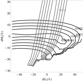
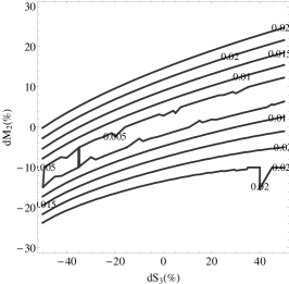
Figure 3: Contour plots that point out what is the best choice for the parameters of an analytic metric so that it matches well a numerical one. The left plot shows the contour plots of the overall mismatch $\sigma_{ij}$ between the analytic and the numerical metric for the $tt$ (black curves) and $t\phi$ components (grey curves), respectively, as a function of the fractional deviation of the quadrupole, $\delta M_{2}$, and the current octupole, $\delta S_{3}$, of the analytic metric from those calculated directly from the numerical metric (assuming the same mass and angular momentum though). Since the contours of the $\sigma_{tt}$ (almost horizontal) are orthogonal to the ones of $\sigma_{t\phi}$ (almost vertical), the combination indicates an optimum choice for the multipole moments of the analytic space-time. That choice is the moments that have zero deviation from the moments of the numerical space-time. The next two contour plots are similar contour plots but the contours correspond to different quantities. The middle one is for the relative difference between the analytic and numerical $R_{\rm{ISCO}}$, while the right one is for the overall difference between the analytic and numerical orbital frequency $\Omega$ (defined analogously to the overall mismatch of the metric components). Both these latter plots are consistent with the first one. All plots correspond to the model $\#15$ for the AU EOS of the models presented by Pappas & Apostolatos (2012) and they give a representative picture of what’s happening with all numerical models that we have computed.

When one attempts to match an analytic solution to a numerical one, it is desirable to find a suitable matching criterion that would be characteristic of the whole structure of the particular numerical space-time, instead of just a finite region of it. That is, the matching should be global and not local. Berti & Stergioulas (2004) have argued that a suitable global condition should be the matching of the first few multipole moments. Indeed, the full set of multipole moments (as defined relativistically by Geroch (1970); Hansen (1974); Fodor, Honselaers & Perjes (1989)) of a stationary and axially symmetric space-time can fully specify the Ernst potential on the axis of symmetry. On the other hand, when the Ernst potential along the axis of symmetry is given, there is a space-time which is unambiguously specified by that Ernst potential as it was shown by Xanthopoulos (1979, 1981); Hauser & Ernst (1981). Thus, the full set of multipole moments are uniquely characterizing a space-time and they can be used as a global matching condition.

When the space-time of a neutron star model is constructed from a numerical algorithm, one can evaluate its mass moments $M,Q,...$ and current moments $J,S_{3},...$ with an accuracy depending on the grid used to present the numerical metric (for further discussion see Berti & Stergioulas (2004), and Pappas & Apostolatos (2012)). Practically, the first few numerically evaluated moments can be used as matching conditions to the analytic space-time. The first four nonzero multipole moments of the two-soliton solution as a function of its parameters $M$, $a$, $b$, $k$ are shown in eq. (2) from which it is clear that once we specify the mass and the angular momentum of the space-time, the parameter $k$ is uniquely determined by the quadrupole moment $Q\equiv M_{2}$ ,while the parameter $b$ is uniquely determined by the current octupole $S_{3}\equiv J_{3}$. Thus, having constrained the four parameters of the two-soliton, we have completely specified an analytic space-time that could be used to describe the exterior of the particular neutron star model. What remains to be seen is how well do the properties of the analytic space-time compare to those of the numerical one.

At this point there is an issue that should be addressed. Having specified the first four non-zero moments of the two-soliton metric, we have fixed all the higher moments of the space-time in a specific manner related to the particular choice of the analytic metric. These higher moments will probably deviate from the ones of the numerical space-time. So the question is, could one make a better choice when trying to match the analytic to the numerical space-time than the one of setting the first four analytic moments exactly equal to the first four numerical moments? To answer this question we have performed the following test. For several numerical models of uniformly rotating neutron stars that we have constructed, we formed a set of two-soliton space-times for each neutron star model that have the same mass $M$ and angular momentum $J$ with the numerical model, while the quadrupoles and the current octupoles of each single two-soliton space-time take the values $M_{2}^{\rm(a)}=M_{2}^{\rm(n)}(1-\delta M_{2})$ and $S_{3}^{\rm(a)}=S_{3}^{\rm(n)}(1-\delta S_{3})$ respectively with various $\delta M_{2}$ and $\delta S_{3}$ values. The quantities $\delta M_{2}$ and $\delta S_{3}$ denote the fractional differences of the corresponding analytic moments of each two-soliton space-time from the numerical one. Then for each one of these sets of moments we calculated the overall mismatch between the analytic and the numerical metric functions, which are defined (see Pappas & Apostolatos (2012)) as

$$\sigma_{ij}=\left[\int_{R_{\rm S}}^{\infty}(g_{ij}^{n}-g_{ij}^{a})^{2}dr\right]^{1/2},$$ (29)

where $R_{\rm S}$ is the radius $r$ at the surface of the star, and have thus constructed contour plots of $\sigma_{ij}$ on the plane of $\delta S_{3}$ and $\delta M_{2}$, like the ones shown in Figure 3. The same type of contour plots were drawn for other quantities as well, like the relative difference of the $R_{\rm ISCO}$ and the overall difference between the analytic and numerical orbital frequency $\Omega$ for circular, equatorial orbits (defined in the same fashion as it was defined the overall metric mismatch in eq. (29)). The contour plots for the particular neutron star model that is shown in Figure 3 are typical of the behavior that we observed in all models. An important result is that the contours for the overall mismatch $\sigma_{tt}$ combined with the contours for $\sigma_{t\phi}$ give us the best choice for matching a numerical to an analytic space-time; namely, the equation of the first four multipole moments between the two space-times. That is because $g_{tt}$ seems to be sensitive mainly in deviations from the numerical quadrupole and thus the contours appear to be approximately horizontal and parallel to the axis of $\delta S_{3}$, while $g_{t\phi}$ seems to be sensitive mainly in deviations from the numerical current octupole and thus the contours appear to be approximately vertical and parallel to the axis of $\delta M_{2}$ (the contours of $\sigma_{t\phi}$ are almost orthogonal to the contours of $\sigma_{tt}$).

We should note here that the exact position of the optimum point in the contour plots of $\sigma_{tt},\sigma_{t\phi}$ did not deviate from $(0,0)$ by more than 3-4 per cent in all cases studied. The largest deviations showed up in some of the fastest rotating models.

The conclusion is that what we expected to be true based on theoretical considerations turns out to be exactly the case after the implementation of the aforementioned test. Therefore in what follows, we will set the first four non-zero multipole moments of the analytic space-time equal to that of the corresponding numerical space-times.

4 Criteria for the comparison of the analytic to the numerical space-time

Once we have constructed the analytic metric, appropriately matched to the corresponding numerical one, we proceed to thoroughly compare the two space-times. In order to do that, we should try again to use criteria that are characteristic of the geometric structure of the whole space-time, and if possible coordinate independent. It would be preferable if these criteria are also related to quantities that are relevant to astrophysical observations. Thus, if two space-times are in good agreement, with respect to these criteria, they could be considered more or less equivalent.On the other hand, such criteria, as well as possible observations associated to them, could be used to distinguish different space-times and consequently different compact objects that are the sources of these space-times.

As a first criterion of comparing the metrics we will use the direct comparison between the analytic and the numerical metric components themselves. Although the metric components are quantities that are not coordinate independent, they have specific physical meanings and can be related to observable quantities. Thus, the $g_{tt}$ component is related to the gravitational redshift of a photon and the injection energy of a particle. The $g_{t\phi}$ component is related to the frame dragging effect, and the angular velocity $\omega=-g_{t\phi}/g_{\phi\phi}$ of the zero angular momentum observers (ZAMOs). Finally the $g_{\phi\phi}$ component is related to the circumference of a circle at a particular radial distance and defines the circumferential radius $R_{\rm circ}=C/2\pi=\sqrt{g_{\phi\phi}}$. Also $g_{\phi\phi}$ together with $g_{rr}$ are used to measure surface areas. So, if the relative difference between the numerical and the analytic metric components

$$g_{tt}=-f,\quad g_{t\phi}=f\omega,$$

$$g_{\phi\phi}=f^{-1}\rho^{2}-f\omega^{2},\quad g_{\rho\rho}=g_{zz}=f^{-1}e^{2\gamma}$$ (30)

is small, then one could consider the analytic metric as a good approximation of the numerical metric.

Another criterion for comparing an analytic to a numerical space-time is the location of the innermost stable circular orbit (ISCO). Particles moving on the equatorial plane are governed by the equation of motion (see for example Ryan (1995))

$$-g_{\rho\rho}\left(\frac{d\rho}{d\tau}\right)^{2}=1-\frac{\tilde{E}^{2}g_{\phi\phi}+2\tilde{E}\tilde{L}g_{t\phi}+\tilde{L}^{2}g_{tt}}{\rho^{2}}\equiv V(\rho),$$ (31)

where $\tilde{E}$ and $\tilde{L}$ are the conserved energy and angular momentum parallel to the axis of symmetry, per unit mass. $V(\rho)$ is an effective potential for the radial motion and in the case of orbits that are circular, we additionally have the conditions $d\rho/d\tau=0$ and $d^{2}\rho/d\tau^{2}=0$, which are equivalent to the conditions for a local extremum of the potential, i.e., $V(\rho)=0$, and $dV(\rho)/d\rho=0$. The radius of the ISCO is evaluated if we further demand the constraint $d^{2}V(\rho)/d\rho^{2}=0$, the physical meaning of which is that the position of the circular orbit is also a turning point of the potential. From these three conditions we can evaluate a specific $\rho_{\rm{ISCO}}$ and from that the $R_{\rm{ISCO}}=\sqrt{g_{\phi\phi}(\rho_{\rm{ISCO}})}$, which we then compare to the corresponding numerical one. The position of the ISCO is of obvious astrophysical interest since it is the inner radius of an accretion disc and recently it has been used to evaluate the rotation parameter of black holes from fitting the continuous spectrum of the accretion disc around them (see work by Shafee et al. (2006)).

Another criterion for comparing the metrics can be the orbital frequency of circular equatorial orbits $\Omega$. The orbital frequency is given by the equation

$$\Omega(\rho)=\frac{-g_{t\phi,\rho}+\sqrt{(g_{t\phi,\rho})^{2}-g_{tt,\rho}g_{\phi\phi,\rho}}}{g_{\phi\phi,\rho}}.$$ (32)

Apart from the orbital frequency one could also use the precession frequencies of the almost circular and almost equatorial orbits, i.e., the precession of the periastron $\Omega_{\rho}$ and the precession of the orbital plane $\Omega_{z}$. These frequencies are derived from the perturbation of the equation of motion

$$-g_{\rho\rho}\left(\frac{d\rho}{d\tau}\right)^{2}-g_{zz}\left(\frac{dz}{d\tau}\right)^{2}=V(\rho,z)$$ (33)

around the circular equatorial orbits. In this expression, $V(\rho,z)$ is the same effective potential which was defined in the second equation of (31) the $z$ dependence of which now has not been omitted as in eq. (31). The perturbation frequencies derived from the above equation are then given with respect to the metric functions as

$$\kappa_{a}^{2} = -\frac{g^{aa}}{2}\left\{(g_{tt}+g_{t\phi}\Omega)^{2}\left(\frac{g_{\phi\phi}}{\rho^{2}}\right)_{,aa}\right.$$ (34)

$$- 2(g_{tt}+g_{t\phi}\Omega)(g_{t\phi}+g_{\phi\phi}\Omega)\left(\frac{g_{t\phi}}{\rho^{2}}\right)_{,aa}$$

$$+ \left.(g_{t\phi}+g_{\phi\phi}\Omega)^{2}\left(\frac{g_{tt}}{\rho^{2}}\right)_{,aa}\right\},$$

where the index $a$ takes either the value $\rho$ or $z$ to obtain the frequency of the radial or the vertical perturbation respectively. These expressions are evaluated on the equatorial plane (at $z=0$); thus they are functions of $\rho$ alone. The corresponding precession frequencies are given by the difference between the orbital frequency and the perturbation frequency:

$$\Omega_{a}=\Omega-\kappa_{a}.$$ (35)

These quantities are quite interesting with respect to astrophysical phenomena as well. More specifically, they can be associated to the orbital motion of material accreting onto a compact object through an accretion disc. These very frequencies have been proposed to be connected to the observed quasi-periodic modulation (QPOs) of the X-ray flux of accretion discs that are present in X-ray binaries (see Stella (2000); van der Klis (2006); Boutloukos et al. (2006); Lamb (2007)).

Finally, the last criterion that we will use to compare metrics is the quantity $\Delta\tilde{E}$ of circular orbits, which expresses the energy difference of the orbits per logarithmic orbital frequency interval as one moves from one circular orbit to the next towards the central object. This quantity is defined as

$$\Delta\tilde{E}=-\Omega\frac{d\tilde{E}}{d\Omega},$$ (36)

where the energy per unit mass $\tilde{E}$ is given by the expression

$$\tilde{E}=\frac{-g_{tt}-g_{t\phi}\Omega}{\sqrt{-g_{tt}-2g_{t\phi}\Omega-g_{\phi\phi}\Omega^{2}}}.$$ (37)

The quantity $\Delta\tilde{E}$ is a measure of the energy that a particle has to lose in order to move from one circular orbit to another closer to the central object so that the frequency increases by one $e$-fold. The quantity, $\Delta\tilde{E}$, is associated to the emission of gravitational radiation and was used by Ryan (1995) to measure the multipole moments of the space-time from gravitational waves emitted by test particles orbiting in that background. The same quantity can also be associated to accretion discs and in particular, in the case of thin discs, it would correspond to the amount of energy that the disc will radiate as a function of the radius from the central object and thus it will be related to the temperature profile of the disc and consequently to the total luminosity of the disc (for a review on accretion discs see Krolik (1999)).

The last set of criteria, i.e., the frequencies and $\Delta\tilde{E}$, are related to specific observable properties of astrophysical systems, in particular of accretion discs around compact objects; thus they are very useful and relevant to astrophysics (for an application see the work by Pappas (2012)).

5 Results of the comparison

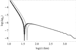
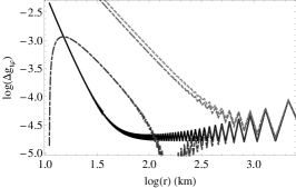
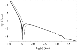
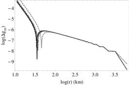
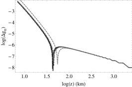
Figure 4: These are the plots of the logarithm of the relative difference of the analytic to the numerical metric components $g_{tt}$, $g_{t\phi}$, $\sqrt{g_{\phi\phi}}=R_{\rm circ}$, and $g_{zz}$ on the equatorial plane, as well as $g_{tt}$ on the axis of symmetry. The plots shown here are indicative of all comparisons performed for all the neutron star models that we have constructed. These particular plots are drawn for the model $\#10$ of the AU EOS, the characteristics of which are presented in Table II of the supplement of Pappas & Apostolatos (2012). Different curves correspond to different metrics, i.e., the two-soliton (solid curve), the Manko et al. solution with the negative root for $b$ (dashed-dotted curve) and the one with the positive root (dashed-double-dotted), and finally the Hartle-Thorne (dotted) metric. In most cases shown here, the Manko et al. curves are on top of the two-soliton curve. The case of the $g_{t\phi}$ component, where the two-soliton curve is almost an order of magnitude below the Manko et al. one for a large interval of radii, is a notable exception. The Hartle-Thorne’s characteristic failure to describe $g_{t\phi}$ is also evident.

The results of the comparison between the analytic and the numerical metrics, describing the exterior of realistic neutron stars, that are presented here is indicative of all comparisons performed for every numerically constructed neutron star model. The models that we have used as a testbed of comparison are briefly presented in the Appendix and are the same models used in Pappas & Apostolatos (2012).

For illustrative reasons we have also plotted comparisons between the numerical and the Manko et al. solution (Manko, Mielke & Sanabria-Gómez (2000)) which was used by Berti & Stergioulas (2004), as well as comparisons between the numerical and the Hartle-Thorne metric (Hartle & Thorne (1968)). The reason for using these two metrics is that on the one hand the Hartle-Thorne metric is considered to be a good approximation of slowly rotating relativistic stars and on the other hand the Manko et al. metric has been shown by Berti & Stergioulas (2004) to be a good approximation for relativistic stars with fast rotation. In cases with slow rotation rates, for which corresponding models of the Manko et al. metric cannot be constructed, we have used only the Hartle-Thorne metric to compare, though. In the case of models with fast rotation besides the Manko et al. metric, we have used the Hartle-Thorne metric as well. for these cases we treated the Hartle-Thorne metric as a three parameter exterior metric, where the three parameters are the mass $M$, the angular momentum $J$ and the reduced quadrupole $q=M_{2}/M^{3}$ of the neutron star. It should be noted that this is not a consistent way to use the Hartle-Thorne metric, since the quadrupole and the angular momentum in the Hartle-Thorne cannot take arbitrary values, while the metric is essentially a two parameter solution (parameterized by the central density of the corresponding slowly rotating star and a small parameter $\varepsilon$ that corresponds to the fraction of the angular velocity of the star relative to the Keplerian angular velocity of the surface of the star) that has to be properly matched to an interior solution following the procedure described by Berti et al. (2004). Here we are taking some leeway in using Hartle-Thorne for fast rotation since it is used simply for illustrative purposes and not in order to draw any conclusions from it.

In Figure 4 we present the comparison of the various analytic metric functions (using the two-soliton, the Manko et al., and the Hartle-Thorne solutions) to the corresponding numerical ones for a single model constructed using the EOS AU (model $\#10$ of the AU EOS the characteristics of which are presented in Table II of the supplement of Pappas & Apostolatos (2012)). The figures display the relative difference between the various analytic and the numerical metric functions $g_{tt},g_{t\phi},\sqrt{g_{\phi\phi}}$ and $g_{zz}=g_{\rho\rho}$ on the equatorial plane, as well as the function $g_{tt}$ on the axis of symmetry.

The general picture we get from these figures is typical for all models constructed using all three equations of state, that is AU, FPS and L. The overall comparison of the two-soliton to the numerical metrics shows that this analytic metric is an excellent substitute of the numerical space-time both for slow and fast rotating models, with an accuracy that is everywhere outside the neutron star always better than about $1/1000$ for all the metric functions (there is an exception to that for the comparison of the $g_{tt}$ metric component right at the pole where for some models it’s fractional difference is a bit smaller than $1/100$). In comparison to the other two analytic metrics discussed above, we see that for the models that a Manko et al. metric can be found, that is for the rapidly rotating neutron stars, both this metric and the two-soliton metric perform very well (actually the Manko et al. solution performs better than Berti & Stergioulas (2004) had initially found as was shown by Pappas & Apostolatos (2012)) and there are only tiny differences between the two-soliton and the Manko et al. analytic metrics. The greatest difference between the two-soliton and the Manko et al. appears to be in the $g_{t\phi}$ component of the metric, where the two-soliton is usually clearly better. This was anticipated because the $g_{t\phi}$ component of the metric is, as we have shown in section 3, more sensitive to the value of $S_{3}$, which can be suitably adjusted in the two-soliton metric, but not in the Manko et al. solution. For the rapidly rotating models the Hartle-Thorne is not such a good representation of the numerical metric as the other two metrics. That also was expected since the Hartle-Thorne metric is not suitable for fast rotation. Hartle-Thorne’s failure is more evident in the $g_{t\phi}$ component of the metric which is consistent with Hartle-Thorne’s vanishing spin octupole $S_{3}$ (in the Appendix we show that $S_{3}=0$ for the Hartle-Thorne metric).

For the slowly rotating models, there are no Manko et al. solutions to compare to the numerical metric, so in these cases the only alternative is the Hartle-Thorne metric. We should say again that the consistent way to calculate the Hartle-Thorne parameters is the one described by Berti et al. (2004), but as it is discussed by Pappas & Apostolatos (2012) the parameters of the Hartle-Thorne metric (specifically the parameter $q$ which is the reduced quadrupole) consistently calculated are in very good agrement with the numerical multipole moments, so these moments were used straightforwardly for the construction of the Hartle-Thorne metric. Again we saw that the two-soliton performs better when compared to the numerical space-time than the Hartle-Thorne metric. We should note though that the problem of Hartle-Thorne’s metric to acurately describe the $g_{t\phi}$ metric component is present even at slow rotation.

Having demonstated the overall superiority of two-soliton, compared to Manko et al. and Hartle-Thorne, to accurately describe the metric functions of any numerical neutron star model, in the following comparisons we will only compare the two-soliton quantities to the corresponding numerical ones.

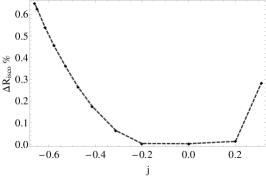
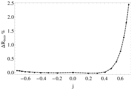
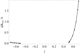
Figure 5: These figures show the relative difference between the numerical and the analytic $R_{\rm{ISCO}}$ for the neutron star models calculated using the AU EOS. The relative difference is shown only for the models that have their ISCO outside the surface of the neutron star. The negative values of $j$ correspond to counter-rotating orbits (retrograde). The data for the co-rotating orbits can be found in Table 2.

The next quantity we have used for comparison is the position of the ISCO. In Figure 5 we present the relative difference between the numerical and the analytic ISCO for all neutron star models constructed with the AU EOS for both prograde and retrograde orbits (the latter are indicated by negative parameter $j\equiv J/M^{2}$). The general conclusion is that for all models constructed using all three EOSs the ISCO of the analytic metric does not deviate by more than 4 per cent from the ISCO of the corresponding numerical model and such deviations are observed for the prograde orbits of the fastest rotating models. We should note that we don’t perform any comparison with numerical models the radius of the surface of which on the equatorial plane is further than the radius of the corresponding ISCO; therefore the points that would correspond to these models are missing from the plots. At this point we should mention that apart from the position of the marginally stable circular orbit for the particles, there is also the position of the unstable photon circular orbit that could also be used as a criterion for comparison. This orbit though is usually, for the prograde case, below the surface of the neutron star (while for the retrograde it is usually outside the star) and it doesn’t have an immediately measurable effect.

We continue to the results of the comparison of the various frequencies associated to the circular orbits on the equatorial plane, i.e., $\Omega,\,\Omega_{\rho},\kappa_{\rho},\Omega_{z}$, and $\kappa_{z}$. The analytic orbital frequency compares very well to the numerical orbital frequency for all the models with the relative difference being in all cases smaller than $\sim 10^{-3}$. This result is very important, since the orbital frequency together with the $R_{\rm{ISCO}}$ are relevant to observations from accretions discs. Typical plots of $\Omega$ and the relative difference between the analytic and the numerical one as functions of the logarithm of the distance from the central object are shown in Figure 6.

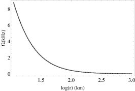
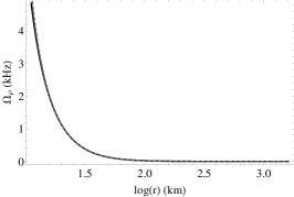
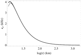
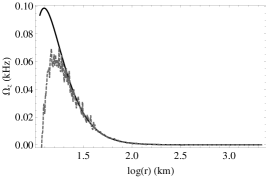
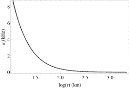
Figure 6: The plots show the various frequencies and the relative difference of the analytic to the corresponding numerical ones. The top row of plots shows on the left the numerical (dotted) and the analytic (solid) orbital frequency $\Omega$ for comparison reasons (they are hardly distinguishable), while on the right it is plotted the logarithm of their relative difference. The middle row shows on the left the numerical (dotted) and analytic (solid) precession frequencies $\Omega_{\rho}$, in the middle the corresponding radial oscillations frequencies $\kappa_{\rho}$ (same correspondence of lines) and on the right the logarithm of the relative difference of the latter oscillation frequencies. Finally the bottom row shows the corresponding plots for the plane precession (left) and the vertical oscillation frequencies (middle), $\Omega_{z}$, and $\kappa_{z}$ respectively, as well as the logarithm of the relative difference of the latter frequencies (right). All plots are for the model $\#10$ of the AU EOS presented by Pappas & Apostolatos (2012).

With regard to the comparison of the radial and vertical perturbation frequencies $\kappa_{\rho}$, and $\kappa_{z}$, respectively, and the corresponding precession frequencies $\Omega_{\rho}$, and $\Omega_{z}$, things are more complicated. These frequencies include second derivatives of the metric functions in their calculation. Consequently the results of the corresponding numerical calculations are plagued by accuracy problems. In particular numerical calculation of the second derivatives induces artificial oscillations in the results. These issues have been discussed earlier by Berti et al. (2004). Following the suggestions of N. Stergioulas, we found two ways to mitigate the problem. The first one is to calculate the frequencies directly in the coordinates that the RNS code produces the metric functions so as to avoid any numerical errors caused by the transformations of the coordinates and the metric functions themselves. Then one would only have to identify the coordinates of the points at which the frequencies are calculated with the corresponding Weyl-Papapetrou coordinates (the calculated frequencies themselves are the frequencies that static observers at infinity measure so they don’t depend on the coordinate system used). The second one is to smooth out these artificial oscillations by taking a three point average of the frequencies. The efficiency of this technique has been tested in the case of the non-rotating models (the exterior of which are described by a Schwarzschild metric) and has been verified to give trustworthy results. Another thing that we should also consider is that in the case of $\kappa_{z}$, the values are very close to the corresponding values of $\Omega$; consequently there is low accuracy in the calculation of the precession frequency $\Omega_{z}=\Omega-\kappa_{z}$ in some cases. That is why we consider as a better indicator of the actual ability of the analytic metric to capture the behavior of the numerical metric, the deviations in the oscillation frequencies $\kappa_{\rho}$ and $\kappa_{z}$, instead of $\Omega_{\rho}$ and $\Omega_{z}$. Nevertheless, we present both the precession and the oscillation frequencies of the analytic metric in comparison to those of the numerical metric, together with the relative difference between the analytic and the numerical oscillation frequencies, in order to get a clearer picture of the comparison. All these plots, again for the model $\#10$ of the AU EOS, the characteristics of which are presented in Table II of the supplement of Pappas & Apostolatos (2012), are shown in Figure 6.

Generally, the relative differences in $\kappa_{\rho}$ between the numerical and the analytic metrics is small and in some cases they could climb up to 10 per cent near the ISCO. This is due to the fact that the radial oscillation frequency tends to zero as the ISCO is approached, causing an increase of the relative difference. In contrast, for $\kappa_{z}$, the relative differences are always below 1 per cent at the ISCO. Now the picture is inverted for the precession frequencies, which is related to the fact that in this case the small quantities are the $\Omega_{z}$’s. The overall picture we obtain is that the analytic frequencies capture quite well the behavior of the numerical frequencies both qualitatively and quantitatively. This is especially evident in the case of the $\kappa_{z}$ frequency where in some cases it becomes greater than the orbital frequency, an effect more prominent in the models of EOS L, which the two-soliton metric captures quite well. The importance of this effect and its relevance to QPOs is further discussed by Pappas (2012).

The final comparison criterion is the quantity $\Delta\tilde{E}$. The numerical computation of this quantity has similar difficulties with the precession frequencies; these issues could be fixed by performing the same tricks to avoid numerical oscillations. In Figure 7 we show for the same model of a rotating neutron star as in the previous cases, the quantity $\Delta\tilde{E}$ computed from the numerical and the analytic metric on the left, and their relative difference on the right. Again we see that the two-soliton metric describes with high accuracy the $\Delta\tilde{E}$ which we obtain numerically from the numerical models. We remind here that this quantity is relevant for the emitted spectrum of a thin accretion disc and its temperature profile, as well as for the efficiency of the disc, i.e., the amount of kinetic energy transformed to radiation.

We close this section with Table 2, where we present for all numerical models of EOS AU (the multipole moments of which are given in the Tables of Pappas & Apostolatos (2012)) the parameters and the type of the two-soliton metric along with a few quantities of astrophysical interest, and specifically their comparison between the ones calculated using the analytic and the numerical space-times. These quantities are, the circumferential radius at the ISCO $R_{\rm{ISCO}}$, the efficiency $\eta=1-\tilde{E}_{\rm{ISCO}}$ of a thin accretion disc (if there was one around the particular neutron star), the orbital frequency at the position of the ISCO $\Omega_{\rm{ISCO}}$ (this is a frequency expected to show up in QPOs if the latter are related to the orbital motion), and finally the vertical oscillation frequency at the ISCO $(\kappa_{z})_{\rm{ISCO}}$ (this could also be related to QPOs). The Table shows that the relative differences between the numerical and the analytic quantities is of the order of 1 per cent or lower.

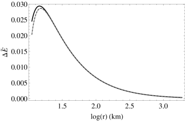
Figure 7: Plots showing the analytic (solid) and numerical (dotted) $\Delta\tilde{E}$ (left) as well as the logarithm of their relative difference (right) for the model $\#10$ of AU EOS presented in Pappas & Apostolatos (2012).

Table 2: For each neutron star model, that was constructed by the RNS code using the AU EOS, we have computed a number of parameters that are related to the particular analytic two-soliton metric which better approximates the numerical metric. These parameters are (i) the type (Case) of the two-soliton space-time that each particular model corresponds to, (ii) the parameters $k$ and $b$ of the two-soliton as well as the spin parameter $j$ and, (iii) the relative difference between the following analytic and numerical quantities: $R_{\rm{ISCO}}$, $\eta$, $\Omega_{\rm{ISCO}}$ and $(\kappa_{z})_{\rm{ISCO}}$, for the models that the ISCO lies outside the surface of the star. The models shown here are the same models presented in Pappas & Apostolatos (2012). The rest of the physical parameters of these models, such as the mass and all the other multipole moments of the models, can be found there. All the relative differences are given as a percentage.

model	Case	$j$	$b$	$k$	$\Delta R_{\rm{ISCO}}$	$\Delta\eta$	$\Delta\Omega_{\rm{ISCO}}$	$(\Delta\kappa_{z})_{\rm{ISCO}}$
			($km$)	($km^{2}$)	(per cent)	(per cent)	(per cent)	(per cent)
1	III	0.	-3.	0	0.003	0.032	0.006	-
2	Ia	0.2015	-0.0784	-0.5271	0.013	0.019	0.003	0.024
3	IIa	0.3126	-0.1305	-1.2503	0.283	0.142	0.027	0.141
4	IIa	0.414	-0.1858	-2.1664	-	-	-	-
5	IIa	0.4749	-0.224	-2.8362	-	-	-	-
6	IIa	0.5297	-0.2626	-3.517	-	-	-	-
7	IIa	0.5789	-0.3014	-4.1972	-	-	-	-
8	IIa	0.617	-0.3351	-4.7738	-	-	-	-
9	IIa	0.651	-0.368	-5.3277	-	-	-	-
10	IIa	0.6618	-0.3793	-5.5114	-	-	-	-
11	III	0.	-3.	0	0.003	-0.021	-0.004	-
12	III	0.194524	-0.0915	-0.1528	-0.021	0.022	0.002	-0.034
13	III	0.309849	-0.1669	-0.4288	-0.018	0.025	0.003	-0.071
14	III	0.406932	-0.2417	-0.8163	0.019	0.03	0.005	0.113
15	III	0.485572	-0.3158	-1.2698	0.148	0.114	0.019	0.04
16	III	0.550214	-0.3897	-1.7658	0.391	0.204	0.035	0.217
17	III	0.603381	-0.4628	-2.279	0.778	0.463	0.077	0.477
18	III	0.645447	-0.5317	-2.7705	1.274	0.83	0.137	0.815
19	III	0.676639	-0.5916	-3.197	1.798	1.205	0.197	1.15
20	III	0.706299	-0.6585	-3.6602	2.453	1.831	0.297	1.638
21	III	0.510282	-0.3726	-0.7958	0.043	0.026	0.005	0.15
22	III	0.510617	-0.3717	-0.8179	0.054	0.046	0.008	0.058
23	III	0.514032	-0.3731	-0.8721	0.063	0.05	0.009	0.031
24	III	0.520506	-0.3789	-0.9409	0.083	0.016	0.004	0.065
25	III	0.547452	-0.4083	-1.1827	0.164	0.072	0.013	0.153
26	III	0.587439	-0.4607	-1.5504	0.346	0.206	0.034	0.164
27	III	0.626593	-0.5214	-1.9574	0.63	0.391	0.064	0.362
28	III	0.659098	-0.5806	-2.3502	0.991	0.645	0.104	0.64
29	III	0.694585	-0.6577	-2.8456	1.551	1.018	0.162	0.948
30	III	0.713165	-0.7054	-3.1406	1.95	1.349	0.214	1.221

6 Conclusions

In this work we have tested whether the four-parameter two-soliton analytic metric, which was derived by Manko, Martin & Ruiz (1995), can be used as a trustworthy approximation for the space-time around all kind of neutron stars. To match the particular analytic metric to a specific neutron star model, which was produced through the numerical code RNS of Stergioulas & Friedman (1995), we have used as matching conditions the first four non-zero multipole moments. Our choice was justified, apart from theoretical reasoning, by comparing the numerical metrics with different analytic metrics produced by slightly varying two of their moments (quadrupole and spin-octupole). The comparison showed clearly that the best matching comes from imposing the condition that the parameters of the analytic metric should be such that the analytic space-time acquires the first four non-vanishing moments of the numerical metric.

Having demonstrated the appropriateness of the matching conditions, we proceeded to compare the various numerical neutron star space-times with the corresponding analytic space-times. To perform the comparison, we have assumed several criteria having in mind that they should correspond to geometric and physical properties of the space-time, with a special interest in physical quantities that could be associated to astrophysical processes that are usually observed from the vicinity of neutron stars.

The result of these comparisons is that the two-soliton space-time can reproduce the properties of the space-time around realistic neutron stars, and in particular it can reproduce all astrophysically interesting properties. Probably the most important fact is that the analytic metric can capture properties of the neutron star space-time that a corresponding Kerr space-time could not, such as the behavior of the precession frequencies of almost circular and almost equatorial orbits. A typical example is shown in Figure 8, where we present the analytic and numerical frequencies of the precession of the orbital plane for a model constructed using the L EOS. The possible importance and implication of this, i.e,. the capability of the two-soliton to capture this particular behavior in contrast to the Kerr geometry, was further discussed in Pappas (2012).

Generally the two-soliton metric can be a very useful tool for studying phenomena that happen around all kind of neutron stars and are quite sensitive to more realistic and accurate geometries than the ones used so far. Relying on a single analytic metric for all neutron stars is practically more favorable than using numerical space-times, or more than one analytic metrics depending on the type of the neutron star. Thus, the two-soliton metric can be further used for more elaborate applications such as the ones explored by Psaltis (2008); Bauböck, Psaltis, Özel & Johannsen (2012); Bauböck, Psaltis & Özel (2012).

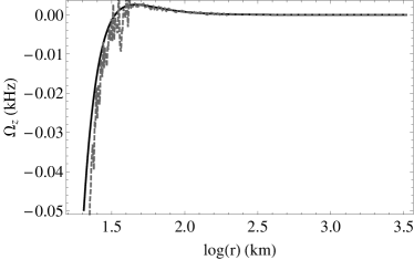
Figure 8: Plot showing the numerical (dotted) and analytic (solid) precession frequencies $\Omega_{z}$ for the model $\#10$ of the L EOS. One can see how the frequencies that are calculated from the analytic metric capture the qualitative behavior of the corresponding numerical frequencies. The parameters (i.e., the multipole moments) for this model can be found in Pappas & Apostolatos (2012).

Appendix A Neutron star models

In order to construct the analytic space-time exterior to a compact object, one has to choose the appropriate multipole moments. For neutron stars, these moments could be computed from numerical models that are constructed with realistic equations of state. There are several schemes developed for numerically integrating stellar models (see Stergioulas & Friedman (1995), and for an extended list of numerical schemes see Stergioulas (2003)). We have used Stergioulas’s RNS code for the construction of the models.

In order to cover more space on the “neutron star parameter space”, we constructed numerical neutron star models with equations of state of varying stiffness. For that purpose we have chosen AU as a typical soft EOS, FPS as a representative moderate stiff EOS, and L to describe stiff EOS. Having the numerical models ready, we proceeded in evaluating their multipole moments according to the algorithm described in Pappas & Apostolatos (2012). The parameters then used to construct the analytic space-time models, i.e., $M,\;a,\;k$, and $b$, are evaluated from the first four multipole moments ($M,\;J,\;M_{2},\;S_{3}$) of each model by inverting equations (2).

For the specifics of the various models chosen here, we have followed Berti & Stergioulas (2004). We have constructed the same constant rest-mass sequences as the ones presented in Berti & Stergioulas (2004) for the corresponding equations of state. For every equation of state, 3 sequences of 10 models were constructed, that corresponded to:

1. a sequence corresponding to a neutron star of $1.4M_{\odot}$ in the non-rotating limit,

2. a sequence terminating at the maximum-mass neutron star in the non-rotating limit,

3. a supermassive sequence that does not terminate at a non-rotating model at its lower rotation limit.

All the sequences end at the mass-shedding limit on the side of fast rotation, i.e., at the limit were the angular velocity of a particle at the equator is equal to the Keplerian velocity at that radius. These sequences are the so called evolutionary sequences.

All the parameters for the computed models can be found in Pappas & Apostolatos (2012).

Appendix B The functions of the two-soliton

In this Appendix we present the full expressions for writing the metric functions of the two-soliton. The determinants that are given in Sec. 2 and appear in the formulas for the metric functions, can be substituted with the following expressions, starting with $E_{\pm}=A\mp B$, where the functions $A,\,B$ are given as:

$$A\!\!\!\! = \!\!\!\!-16dk\left(r_{-}r_{+}+R_{-}R_{+}\right)M^{2}$$ (38)

$$- \!\!\!\!\left[A_{1}^{-}\left(R_{-}r_{+}+r_{-}R_{+}\right)-A_{2}^{-}\left(R_{-}r_{+}-r_{-}R_{+}\right)\right]\kappa_{+}^{2}$$

$$+ \!\!\!\!\left[A_{1}^{+}\left(r_{-}R_{-}+r_{+}R_{+}\right)-A_{2}^{+}\left(r_{-}R_{-}-r_{+}R_{+}\right)\right]\kappa_{-}^{2},$$

$$A_{1}^{\pm}\!\!\!\! = \!\!\!\!\left(4(a-b)^{2}(ab\pm d-k)-4((a-2b)b\pm d)M^{2}\right),$$ (39)

$$A_{2}^{\pm}\!\!\!\! = \!\!\!\!4i\left((a-b)(ab\pm d-k)-bM^{2}\right)\kappa_{\pm},$$ (40)

$$B\!\!\!\! = \!\!\!\!2\kappa_{-}\kappa_{+}M\left[\left(R_{+}-R_{-}\right)B_{1}^{-}+\left(r_{-}-r_{+}\right)B_{1}^{+}\right.$$ (41)

$$+ \!\!\!\!\left.\left(R_{-}+R_{+}\right)B_{2}^{-}-\left(r_{-}+r_{+}\right)B_{2}^{+}\right],$$

$$B_{1}^{\pm}\!\!\!\! = \!\!\!\!i\left(2k(a-b)+b\left(M^{2}-a^{2}+b^{2}\pm\kappa_{-}\kappa_{+}\right)\right)$$ (42)

$$\times \!\!\!\!\left(\kappa_{+}\pm\kappa_{-}\right),$$

$$B_{2}^{\pm}\!\!\!\! = \!\!\!\!2d\left(M^{2}-a^{2}+b^{2}\pm\kappa_{-}\kappa_{+}\right).$$ (43)

The determinant $H$ can be substituted as $H=-L$, where $L$ is given by the expression,

$$L\!\!\!\! = \!\!\!\!\left(r_{-}r_{+}+R_{-}R_{+}\right)L_{1}+\left(r_{-}+R_{-}+r_{+}+R_{+}\right)L_{2}$$ (44)

$$- \!\!\!\!\left(r_{-}-R_{-}+r_{+}-R_{+}\right)L_{3}+\left(r_{-}R_{-}-R_{+}r_{+}\right)L_{5}^{-}$$

$$+ \!\!\!\!(r_{-}-r_{+}+R_{-}-R_{+})L_{4}^{-}+\left(r_{-}R_{+}-R_{-}r_{+}\right)L_{5}^{+}$$

$$+ \!\!\!\!(r_{-}-r_{+}-R_{-}+R_{+})L_{4}^{+}+\left(R_{-}r_{+}+r_{-}R_{+}\right)L_{6}^{+}$$

$$+ \!\!\!\!\left(R_{-}r_{-}+r_{+}R_{+}\right)L_{6}^{-},$$

$$L_{1}\!\!\!\! = \!\!\!\!-16dk(ia-ib+M-z)M^{2},$$ (45)

$$L_{2}\!\!\!\! = \!\!\!\!i4dM(a+iM)\left[M^{4}-2\left(a^{2}-b^{2}-2k\right)M^{2}\right.$$ (46)

$$+ \!\!\!\!\left.(a-b)^{2}\left((a+b)^{2}-4k\right)\right],$$

$$L_{3}\!\!\!\! = \!\!\!\!4dM\left[ia^{3}-Ma^{2}-i\left(b^{2}+M^{2}+2k\right)a+M^{3}\right.$$ (47)

$$+ \!\!\!\!\left.2ibk+b^{2}M\right]\kappa_{-}\kappa_{+},$$

$$L_{4}^{\pm}\!\!\!\! = \!\!\!\!4\kappa_{\mp}M\left\{ibM^{5}+abM^{4}\right.$$ (48)

$$- \!\!\!\!i\left(2ba^{2}-ka-b\left(b^{2}\pm d+2k\right)\right)M^{3}$$

$$- \!\!\!\!\left(2ba^{3}-ka^{2}-b\left(b^{2}\pm d+3k\right)a\right.$$

$$+ \!\!\!\!\left.k\left(2b^{2}\mp d+k\right)\right)M^{2}$$

$$+ \!\!\!\!\left(2k^{2}-\left(a^{2}+3ba\mp 2d\right)k+b(a+b)\left(a^{2}\mp d\right)\right)$$

$$\times \!\!\!\!i(a-b)M$$

$$+ \!\!\!\!\left.(a-b)(ab-k)\left((a+b)\left(a^{2}\mp d\right)+(b-3a)k\right)\right\},$$

$$L_{5}^{\pm}\!\!\!\! = \!\!\!\!+4i\left[b(M-z)a^{4}+\left(b^{2}\mp d-k\right)(M-z)a^{3}\right.$$ (49)

$$+ \!\!\!\!\left((z-M)b^{3}+iM^{2}b^{2}\right.$$

$$+ \!\!\!\!\left.\left(2M^{2}\pm d+5k\right)(z-M)b\mp idM^{2}\right)a^{2}$$

$$+ \!\!\!\!\left((z-M)b^{4}+\left(M^{2}\mp d-5k\right)(z-M)b^{2}\right.$$

$$- \!\!\!\!\left.4ikM^{2}b+(k\pm d)\left(M^{2}+4k\right)(M-z)\right)a$$

$$- \!\!\!\!ib^{4}M^{2}-ib^{2}M^{2}\left(M^{2}\mp d-2k\right)$$

$$+ \!\!\!\!iM^{2}\left(2k(k\pm d)\pm dM^{2}\right)+b\left(b^{2}\left(M^{2}\pm d+k\right)\right.$$

$$+ \!\!\!\!\left.\left.\left(M^{4}+(k\pm d)M^{2}-4k(k\pm d)\right)\right)(M-z)\right]\kappa_{\mp},$$

$$L_{6}^{\pm}\!\!\!\! = \!\!\!\!\pm 4\left[b(M-z)a^{5}+((k\pm d)(z-M)+ibM^{2})a^{4}\right.$$ (50)

$$+ \!\!\!\!\left(2(z-M)b^{3}+2\left(M^{2}+2k\right)(z-M)b\right.$$

$$- \!\!\!\!\left.ikM^{2}\right)a^{3}$$

$$+ \!\!\!\!\left(-2iM^{2}b^{3}+2(5k\pm d)(M-z)b^{2}\right.$$

$$- \!\!\!\!i\left(2M^{4}+3kM^{2}\right)b$$

$$+ \!\!\!\!\left.\left((k\pm 2d)M^{2}+4k(k\pm d)\right)(M-z)\right)a^{2}$$

$$+ \!\!\!\!\left\{(M-z)b^{5}-2\left(2k-M^{2}\right)(M-z)b^{3}\right.$$

$$+ \!\!\!\!7ikM^{2}b^{2}+\left(M^{4}+4kM^{2}-8k(k\pm d)\right)(M-z)b$$

$$+ \!\!\!\!\left.ikM^{2}\left(M^{2}+2(k\pm d)\right)\right\}a$$

$$+ \!\!\!\!ib^{5}M^{2}-ib^{3}\left(3k-2M^{2}\right)M^{2}$$

$$+ \!\!\!\!ibM^{2}\left(M^{4}+3kM^{2}-2k(k\pm d)\right)$$

$$+ \!\!\!\!\left(M^{2}\left(2k(k\pm d)\pm dM^{2}\right)+b^{4}(k\pm d)\right)(z-M)$$

$$+ \!\!\!\!\left.b^{2}\left(4k(k\pm d)-(3k\pm 2d)M^{2}\right)(M-z)\right].$$

The determinant $G$ can be expressed as $G=-E$, where $E$ is given by the expressions,

$$E\!\!\!\! = \!\!\!\!E_{1}\left(r_{-}r_{+}+R_{-}R_{+}\right)+E_{2}\left(r_{-}+R_{-}+r_{+}+R_{+}\right)$$ (51)

$$+ \!\!\!\!E_{3}\left(r_{-}-R_{-}+r_{+}-R_{+}\right)+E_{4}^{+}(r_{-}R_{+}-R_{-}r_{+})$$

$$+ \!\!\!\!E_{4}^{-}(r_{-}R_{-}-r_{+}R_{+})+E_{5}^{+}(R_{-}r_{+}+r_{-}R_{+})$$

$$+ \!\!\!\!E_{5}^{-}(r_{-}R_{-}+r_{+}R_{+})+E_{6}^{+}(r_{-}-r_{+}-R_{-}+R_{+})$$

$$+ \!\!\!\!E_{6}^{-}(r_{-}-r_{+}+R_{-}-R_{+}),$$

$$E_{1}\!\!\!\! = \!\!\!\!16dk(-ia+ib+M)M^{2},$$ (52)

$$E_{2}\!\!\!\! = \!\!\!\!4d\kappa_{-}^{2}\kappa_{+}^{2}(ia+M-z)M,$$ (53)

$$E_{3}\!\!\!\! = \!\!\!\!4d\left[2ik(a-b)+\left(b^{2}+M^{2}-a^{2}\right)(M-z+ia)\right]$$ (54)

$$\times \!\!\!\!\kappa_{-}\kappa_{+}M,$$

$$E_{4}^{\pm}\!\!\!\! = \!\!\!\!-4i\left[bM^{4}+i\left(b^{2}\mp d\right)M^{3}\right.$$ (55)

$$- \!\!\!\!(a+b)\left(2ab-b^{2}\mp d-k\right)M^{2}$$

$$- \!\!\!\!i\left(2k^{2}+2\left(b^{2}-2ab\pm d\right)k\right.$$

$$+ \!\!\!\!\left.(a^{2}-b^{2})\left(b^{2}\mp d\right)\right)M$$

$$+ \!\!\!\!\left.(a-b)\left((a+b)^{2}-4k\right)(ab\mp d-k)\right]\kappa_{\mp}M,$$

$$E_{5}^{\pm}\!\!\!\! = \!\!\!\!\pm 4M\left[ibM^{5}-(ab\mp d)M^{4}\right.$$ (56)

$$- \!\!\!\!i\left(-2b^{3}+2a^{2}b-3kb-ak\right)M^{3}$$

$$+ \!\!\!\!\left(2k^{2}-\left(a^{2}+4ba-3b^{2}\mp 2d\right)k\right.$$

$$+ \!\!\!\!\left.2(a^{2}-b^{2})(ab\mp d)\right)M^{2}$$

$$+ \!\!\!\!i(a-b)\left((a-b)b(a+b)^{2}+2k^{2}\right.$$

$$- \!\!\!\!\left.\left(a^{2}+4ba-3b^{2}\mp 2d\right)k\right)M$$

$$- \!\!\!\!\left.(a-b)^{2}\left((a+b)^{2}-4k\right)(ab\mp d-k)\right],$$

$$E_{6}^{\pm}\!\!\!\! = \!\!\!\!4\kappa_{\mp}M\left\{ba^{5}-(k+ib(M-z))a^{4}\right.$$ (57)

$$- \!\!\!\!\left(b^{3}+\left(2M^{2}\pm d+3k\right)b-ik(M-z)\right)a^{3}$$

$$+ \!\!\!\!\left(i(M-z)b^{3}+5kb^{2}+i\left(\pm d+2\left(M^{2}+k\right)\right)\right.$$

$$\times \!\!\!\!\left.(M-z)b+k\left(M^{2}\pm d+3k\right)\right)a^{2}$$

$$+ \!\!\!\!\left(\left(M^{2}\pm d-k\right)b^{3}-3ik(M-z)b^{2}\right.$$

$$+ \!\!\!\!\left(M^{4}+(3k\pm d)M^{2}-4k^{2}\right)b$$

$$- \!\!\!\!\left.ik\left(M^{2}+2(k\pm d)\right)(M-z)\right)a$$

$$- \!\!\!\!(k\mp d)kM^{2}+b^{2}k\left(-2M^{2}\mp d+k\right)$$

$$- \!\!\!\!ib^{3}\left(M^{2}\pm d\right)(M-z)$$

$$- \!\!\!\!\left.ib\left(M^{4}+(2k\pm d)M^{2}-2k(k\pm d)\right)(M-z)\right\},$$

and finally the determinant $K_{0}$ can be expressed as

$$K_{0}=-16d\kappa_{-}^{2}\kappa_{+}^{2}.$$ (58)

In order to get the metric functions one should substitute these expressions to the equations (11-14). We should note here that the above expressions are not equal to the corresponding determinants since a common factor to all the determinants, i.e., the quantity $\prod_{k=1}^{n}e_{k}e^{*}_{k}$, has been simplified out of the expressions.

Appendix C Transformation to Weyl-Papapetrou coordinates for a general metric

As we have mentioned, a stationary and axially symmetric space-time $g_{\mu\nu}(x^{\mu})$ can be cast in the form of the Papapetrou line element (1)

$$ds^{2}=-f(dt-\omega d\phi)^{2}+f^{-1}\left(e^{2\gamma}(d\rho^{2}+dz^{2})+\rho^{2}d\phi^{2}\right),$$

by an appropriate coordinate transformation, where the metric functions are functions of the Weyl-Papapetrou coordinates $(\rho,z)$. These coordinates as expressed as functions of the previous coordinates $x^{\mu}$ are harmonic conjugate functions. That is, the coordinate $\rho(x^{\mu})$ is defined as $\rho^{2}=(g_{t\phi})^{2}-g_{tt}g_{\phi\phi}$ and satisfies the Laplace equation while $z(x^{\mu})$ is it’s harmonic conjugate. Thus the integrability conditions for $z$ are the Cauchy-Riemann conditions which can be used to calculate that coordinate. In an earlier work (see Pappas & Apostolatos (2008)) we have shown the correct way to integrate these conditions when one has to transform a metric given in quasi-isotropic coordinates

$$ds^{2}=-e^{2\nu}dt^{2}+e^{2\psi}\left(d\phi-\omega dt\right)^{2}+e^{2\mu}\left(dr^{2}+r^{2}d\theta^{2}\right),$$ (59)

which are commonly used in numerical integrations of the Einstein field equations, to the Papapetrou form. In that case, the quasi-isotropic coordinates, $r,\theta$ enter the metric in a way that can be easily cast in a cartesian form and thus the Cauchy-Riemann conditions are given from the usual expressions

$$\frac{\partial z}{\partial\varpi}=-\frac{\partial\rho}{\partial\zeta},$$

$$\frac{\partial z}{\partial\zeta}=\frac{\partial\rho}{\partial\varpi},$$

where we have defined the cartesian coordinates $\varpi=r\sin\theta=r\sqrt{1-\mu^{2}},\;\zeta=r\cos\theta=r\mu$.

In the case of a metric given in a general form though, like the Hartle-Thorne metric, the Cauchy-Riemann conditions can not be used as given in the previous equations. So, one has to calculate the general form of these conditions. The general expressions for the Cauchy-Riemann conditions can be evaluated from the orthogonality condition that the functions $\rho(r,\theta)$ and $z(r,\theta)$ must satisfy. Thus, for a metric given in the form

$$ds^{2}=g_{tt}dt^{2}+2g_{t\phi}dtd\phi+g_{rr}dr^{2}+g_{\theta\theta}d\theta^{2}+g_{\phi\phi}d\phi^{2},$$ (60)

the orthogonality condition between $\rho$ and $z$ is $\nabla\rho\cdot\nabla z=0$, which gives the expressions for the Cauchy-Riemann conditions

$$\frac{\partial z}{\partial r}=\sqrt{\frac{g_{rr}}{g_{\theta\theta}}}\frac{\partial\rho}{\partial\theta},$$ (61)

$$\frac{\partial z}{\partial\theta}=-\sqrt{\frac{g_{\theta\theta}}{g_{rr}}}\frac{\partial\rho}{\partial r},$$ (62)

where we have expressed the conditions in the $r,\theta$ coordinates and the function $\rho(r,\theta)$ is defined as

$$\rho(r,\theta)=\sqrt{(g_{t\phi})^{2}-g_{tt}g_{\phi\phi}}.$$ (63)

These general Cauchy-Riemann conditions are used in the same way as prescribed in Pappas & Apostolatos (2008) in order to evaluate the $z$ coordinate for the Hartle-Thorne metric and then compare the latter metric with the numerical metric and the two-soliton metric on the axis of symmetry. The metric functions given by the metric in the general form can be directly associated to the metric functions in the Papapetrou line element (1) by comparing the corresponding $g_{tt},~{}g_{t\phi}$ and $g_{\phi\phi}$ values. The only component that needs to be evaluated then is the $g_{\rho\rho}=g_{zz}$ and it is given by the equation

$$g_{\rho\rho}=g_{zz}=f^{-1}e^{2\gamma}=\left(\frac{1}{g_{rr}}(\rho_{,r})^{2}+\frac{1}{g_{\theta\theta}}(\rho_{,\theta})^{2}\right)^{-1}.$$ (64)

Appendix D The Hartle-Thorne metric.

This is a metric produced by Hartle & Thorne (1968) as an expansion up to order $O(\varepsilon^{3})$, where $\varepsilon=\Omega/\Omega_{*}$ is a parameter that characterizes the rotation of a star, and corresponds to the exterior space-time of slowly rotating relativistic stars ($\Omega_{*}=\sqrt{M/R^{3}}$ is the Kepler limit). The components of the metric can be found in Berti et al. (2004) and are given by the expressions,

$$g_{tt} = -\left(1-\frac{2M}{r}\right)\left(1+j^{2}F_{1}-qF_{2}\right),$$ (65)

$$g_{rr} = \left(1-\frac{2M}{r}\right)^{-1}\left(1+j^{2}G_{1}+qF_{2}\right),$$ (66)

$$g_{\theta\theta} = r^{2}\left(1+j^{2}H_{1}-qH_{2}\right),$$ (67)

$$g_{\phi\phi} = \sin^{2}\theta g_{\theta\theta},$$ (68)

$$g_{t\phi} = \left(\frac{2jM^{2}}{r}\right)sin^{2}\theta,$$ (69)

where

$$L = 80M^{6}+8r^{2}M^{4}+10r^{3}M^{3}+20r^{4}M^{2}$$

$$- 45r^{5}M+15r^{6},$$

$$p = \frac{1}{8Mr^{4}(r-2M)},$$

$$W = \left(48M^{6}-8rM^{5}-24r^{2}M^{4}-30r^{3}M^{3}\right.$$

$$- \left.60r^{4}M^{2}+135r^{5}M-45r^{6}\right)u^{2}$$

$$+ \left(16M^{5}+8rM^{4}-10r^{3}M^{2}-30r^{4}M+15r^{5}\right)$$

$$\times (r-M),$$

$$A_{1} = \frac{15r(r-2M)\left(1-3u^{2}\right)\ln\left(\frac{r}{r-2M}\right)}{16M^{2}},$$

$$A_{2} = \frac{15\left(r^{2}-2M^{2}\right)\left(3u^{2}-1\right)\ln\left(\frac{r}{r-2M}\right)}{16M^{2}},$$

$$F_{1} = -pW+A_{1},$$

$$F_{2} = 5pr^{3}(r-M)\left(2M^{2}+6rM-3r^{2}\right)\left(3u^{2}-1\right)-A_{1},$$

$$G_{1} = p\left(-72rM^{5}-3\left(L-56M^{5}r\right)u^{2}+L\right)-A_{1},$$

$$H_{1} = \frac{\left(16M^{5}+8rM^{4}-10r^{3}M^{2}+15r^{4}M+15r^{5}\right)}{8Mr^{4}}$$

$$\times \left(1-3u^{2}\right)+A_{2},$$

$$H_{2} = \frac{5\left(2M^{2}-3rM-3r^{2}\right)\left(1-3u^{2}\right)}{8Mr}-A_{2},$$

with $u=\cos\theta$. We will now try to evaluate the first five multipole moments of the Hartle-Thorne space-time, following Ryan (1995). From the metric functions one can calculate the rotation frequency of circular equatorial orbits, which is given by equation (32). $\Omega$ can be expressed with respect to a new parameter $\upsilon=(M\Omega)^{1/3}$. This new parameter is a function of $r$, which can in turn be expressed as a function of another new parameter, $x=(M/r)^{1/2}$. Then the parameter $\upsilon$ can be expanded as a series in $x$. This series can then be inverted and thus the parameter $x$ can be expressed as a power series in $\upsilon$. Similarly, we can calculate the energy per mass, $\tilde{E}$, of a test particle in circular orbit (37) as a function of the parameter $x$. This quantity can then be expressed as an expansion on $x$ which by substituting the previously obtained power series can then be expressed as a series expansion in $\upsilon$. From that, one can calculate the invariant quantity

$$\Delta\tilde{E}=-\Omega\frac{d\tilde{E}}{d\Omega}=-\frac{\upsilon}{3}\frac{d\tilde{E}}{d\upsilon},$$ (70)

which is related to the multipole moments of the space-time as they are given by Ryan (1995). After following all the previously mentioned calculations, the expansion of the above expression is,

$$\Delta\tilde{E} = \frac{\upsilon^{2}}{3}-\frac{\upsilon^{4}}{2}-\frac{20j\upsilon^{5}}{9}+\left(q-\frac{27}{8}\right)\upsilon^{6}-\frac{28j\upsilon^{7}}{3}$$ (71)

$$+ \left(\frac{80j^{2}}{27}+\frac{70q}{9}-\frac{225}{16}\right)\upsilon^{8}+\left(-6qj-\frac{81j}{2}\right)\upsilon^{9}$$

$$+\left(\frac{115j^{2}}{18}+\frac{35q^{2}}{12}+\frac{935q}{24}-\frac{6615}{128}\right)\upsilon^{10}$$

$$+ \left(-\frac{1408j^{3}}{243}-\frac{572qj}{27}-165j\right)\upsilon^{11}+O(\upsilon^{12}).$$

From comparing Ryan’s expressions to this expansion, we see that the Hartle-Thorne metric, as given by Berti, has a rotation parameter $j$ defined as $j=-J/M^{2}$, a quadrupole parameter $q=Q/M^{3}$ and the following moments $S_{3},\;M_{4}$ are equal to zero. The above expansion seems to be consistent with the aforementioned multipole moments up to $O(\upsilon^{11})$.

References

- Berti & Stergioulas (2004) Berti E., Stergioulas N., 2004, MNRAS, 350 1416
- Berti et al. (2004) Berti E., White F., Maniopoulou A., Bruni M., 2005, MNRAS, 358, 923
- Boutloukos et al. (2006) Boutloukos S., van der Klis M., Altamirano D., Klein-Wolt M., Wijnands R., Jonker P.G., Fender R.P., 2006, ApJ, 653, 1435
- Bauböck, Psaltis, Özel & Johannsen (2012) Bauböck M., Psaltis D., Özel F., Johannsen T., 2012, ApJ, 753, 175
- Bauböck, Psaltis & Özel (2012) Bauböck M., Psaltis D., Özel F., preprint (arXiv:1209.0768[astro-ph])
- Ernst (1968a) Ernst F.J., 1968, Phys. Rev., 167, 1175
- Ernst (1968b) Ernst F.J., 1968, Phys. Rev., 168, 1415
- Fodor, Honselaers & Perjes (1989) Fodor G., Honselaers C., Perjes Z., 1989, J. Math. Phys., 30, 2252
- Geroch (1970) Geroch R., 1970, J. Math. Phys., 11, 2580
- Hansen (1974) Hansen R.O., 1974, J. Math. Phys., 15, 46
- Hartle & Thorne (1968) Hartle J. B., Thorne K. S., 1968, ApJ, 153, 807
- Hauser & Ernst (1981) Hauser I.,Ernst F. J., 1981, J. Math. Phys., 22, 1051
- Krolik (1999) Krolik J.H., 1999, Active galactic nuclei: from the central black hole to the galactic environment. Princeton Univ. Press, Princeton, NJ
- Lamb (2007) Lamb F.K., 2007, preprint (arXiv:0705.0030[astro-ph])
- Lukes-Gerakopoulos (2012) Lukes-Gerakopoulos G., 2012 Phys. Rev. D, 86, 044013
- Manko & Sibgatulin (1993) Manko V.S., Sibgatullin N.R., 1993, Class. Quantum Grav., 10, 1383
- Manko, Martin & Ruiz (1995) Manko V.S., Martin J., Ruiz J.E., 1995, J. Math. Phys., 36, 3063
- Manko, Mielke & Sanabria-Gómez (2000) Manko V. S., Mielke E. W., Sanabria-Gómez J. D., 2000, Phys. Rev. D, 61, 081501
- Pachón, Rueda & Sanabria-Gómez (2006) Pachón L.A., Rueda J.A., Sanabria-Gómez J.D., 2006, Phys. Rev. D, 73, 104038
- Pachón, Rueda & Valenzuela-Toledo (2012) Pachón L.A., Rueda J.A., Valenzuela-Toledo C.A., 2012, ApJ, 756, 82
- Papapetrou (1953) Papapetrou A., 1953, Ann. Phys., 12, 309
- Pappas (2009) Pappas G., 2009, Journal of Physics: Conference Series, 189, 012028
- Pappas (2012) Pappas G., 2012, MNRAS, 422, 2581
- Pappas & Apostolatos (2008) Pappas G., Apostolatos T.A., 2008, Class. Quantum Grav., 25, 228002
- Pappas & Apostolatos (2012) Pappas G., Apostolatos T.A., 2012, Phys. Rev. Lett., 108, 231104
- Psaltis (2008) Psaltis D., 2008, Living Reviews in Relativity, 11, 9
- Ruiz, Manko & Martin (1995) Ruiz E., Manko V.S., Martin J., 1995, Phys. Rev. D, 51, 4192
- Ryan (1995) Ryan F.D., 1995, Phys. Rev. D, 52, 5707
- Shafee et al. (2006) Shafee R., McClintock J. E., Narayan R., Davis S. W., Li L.-X., Remillard R. A., ApJ, 636, L113
- Sibgatulin (1984) Sibgatullin N.R., 1991, Oscilations and Waves in Strong Gravitational and Electromagnetic Fields. Springer, Berlin [original in Russian, 1984, Nauka, Moscow]
- Sotiriou & Pappas (2005) Sotiriou T.P., Pappas G., 2005, Journal of Physics: Conference Series, 8, 23
- Stella (2000) Stella L., 2000, preprint (astro-ph/0011395)
- Stergioulas (2003) Stergioulas N., 2003, Living Reviews in Relativity, 6, http://relativity.livingreviews.org/lrr-2003-3
- Stergioulas & Friedman (1995) Stergioulas N., Friedman J.L., 1995, ApJ, 444, 306
- Stute & Camenzind (2002) Stute M., Camenzind M., 2002, MNRAS, 336, 831
- Teichmüller, Fröb & Maucher (2011) Teichmüller C., Fröb M.B., Maucher F., 2011, Class. Quantum Grav., 28 155015
- van der Klis (2006) van der Klis M., 2006, in Lewis W.H.G., van der Klis M., eds, Compact Stellar X-Ray Sources. Cambridge Univ. Press, p. 39
- Xanthopoulos (1979) Xanthopoulos, B. C., 1979, J. Phys. A: Math. Gen., 12, 1025
- Xanthopoulos (1981) Xanthopoulos, B. C., 1981, J. Math. Phys., 22, 1254