Matching markers and unlabeled configurations in protein gels

Abstract

Unlabeled shape analysis is a rapidly emerging and challenging area of statistics. This has been driven by various novel applications in bioinformatics. We consider here the situation where two configurations are matched under various constraints, namely, the configurations have a subset of manually located “markers” with high probability of matching each other while a larger subset consists of unlabeled points. We consider a plausible model and give an implementation using the EM algorithm. The work is motivated by a real experiment of gels for renal cancer and our approach allows for the possibility of missing and misallocated markers. The methodology is successfully used to automatically locate and remove a grossly misallocated marker within the given data set.

, and t1Supported by a case studentship funded by the Engineering and Physical Science Research Council and Central Science Laboratories, York, UK.

1 Introduction

1.1 Western Blots

Our motivating application concerns gel techniques used to identify proteins present in human tissue. First, two-dimensional electrophoresis (2-DE) is used to separate all the proteins extracted from a cell. The 2-DE gel is then probed with serum which contains antibodies that will bind to specific proteins. The image of a Western Blot will contain only the location (and intensity) of proteins that have a bound antibody. We can think of Western Blots as containing only a subset of the proteins that are displayed on 2-DE images. The extra step necessary to create a Western Blot allows a further level of variability within the final image. The reproducibility of Western Blots is therefore even more challenging than that of 2-DE images. To help align Western Blots, suitable marker proteins are experimentally determined and are generally expected to be present in all blots under investigation. A stain is applied to each blot which will highlight all proteins present, therefore enabling an expert to manually locate the suitable markers. Figure 1 shows an annotated Western Blot image which shows the markers (with the acidity and mass measurements associated with these points) and further points detected by an image analyzer. The markers are used to align the blots by minimizing a sum of squared euclidean distances (usually not the acidity and mass measurements). In some cases, fine adjustments to alignments are made using various heuristic techniques. See, for example, Forgber et al. (2009) and Zvelebil and Baum [(2007), pages 613–620] for more details.

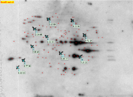
Figure 1: Western Blot image with red crosses depicting the subject-treatment specific nonmarkers. The larger black crosses indicate the labeled markers, with their acidity and mass measurements (not spatial coordinates) highlighted beneath.

Considering the large scope for variation between images and the often vast number of proteins located in a comparatively small area, visual examination to analyze or compare images, although often informative, can be extremely difficult and conclusions unreliable. Visual comparison can also be extremely repetitive and laborious for the expert making the comparisons. Statistical and computational analysis is essential to the result accuracy and reduction of expert manual labor. The main aim is to locate a biomarker whose mere presence can be used to measure the progress of disease or treatment effects. In the case of the gel data, a point becomes a biomarker if it is found to have this property. The intensity of a biomarker, indicated by the intensity of the mark on the image, can also provide information about the disease progression or treatment effect, but this is beyond the scope of this paper.

1.2 Unlabeled configuration matching

In the more general setting, the problem is to match two sets—usually of unequal size—of points, in which the correspondence (matching) of the points is unknown. The solution will include the transformation required to align the sets, a list of correspondences which map (some of) the points, and will penalize solutions with many unmatched points, allowing for a trade-off in the goodness of fit in the aligned points.

Approaches to closely related problems include the RANSAC algorithm [Fischler and Bolles (1981)], nonrigid point matching using thin-plate splines [Chui and Rangarajan (2003)], a correlation-based approach using kernels [Tsin and Kanade (2004), Chen (2011)], nonaffine matching of distributions [Glaunes, Trouvé and Younes (2004)] and the Iterative Closest Point Algorithm [Besl and McKay (1992)] for the registration of various representations of shapes. All of these methods avoid making distributional assumptions, with a consequence that probabilistic statements are then difficult to make. By contrast, Czogiel, Dryden and Brignell (2011), Dryden, Hirst and Melville (2007), Kent, Mardia and Taylor (2010a), Taylor, Mardia and Kent (2003) and Green and Mardia (2006) use statistical models to obtain solutions. These latter papers all use examples drawn from protein bioinformatics; a review is given by Green et al. (2010).

In this paper we address a more specific problem in which each configuration contains a subset of points (“markers”) whose labels correspond with high probability, with the remaining points having arbitrary labels (nonmarkers) as before. Suppose we have two configurations of observed landmarks in $d$ dimensions: markers given by $x_{j}$, $j=1,\ldots,K$ and $\mu_{i}$, $i=1,\ldots,K$, and nonmarkers $\mu_{i}$, $i=K+1,\ldots,K+m$ and $x_{j}$, $j=K+1,\ldots,K+n$. These are represented as matrices $x((K+n)\times d)$ and $\mu((K+m)\times d)$ in which $K$ is usually smaller than $m$ and $n$. In our model, the markers (the spatial coordinates of the large black crosses in Figure 1) $\mu_{i}$ and $x_{i}$ for $i=1,\ldots,K$ have been identified by an expert to correspond to the same proteins (referred to as a “points” hereafter). However, these are labeled with some uncertainty, so true correspondence is likely but not guaranteed. So it is possible, for example, that markers in $\mu$ could correspond to nonmarkers in $x$, or have no correspondence at all. For $\mu_{i}$ and $x_{j}$ with $i,j>K$, (the spatial coordinates of the red crosses in Figure 1) we have no prior information about correspondence probabilities.

1.3 Statistical model

A statistical model in the general setting involves three main components (see Figure 2): [(a)]

A group $\mathcal{G}$, say, on $\mathbb{R}^{d}$ representing the permitted transformations ($g$) on (a subset of the landmarks of) $\mu$ to bring it close to (a subset of the landmarks of) $x,g\in\mathcal{G}$.

A matching matrix $M$, say, identifies which elements of $x$ correspond to which elements of $\mu$ for the markers as well as unlabeled points.

An error model indicating how close the elements of $x$ and $\mu$ will be, after the correct transformation and labeling are used.

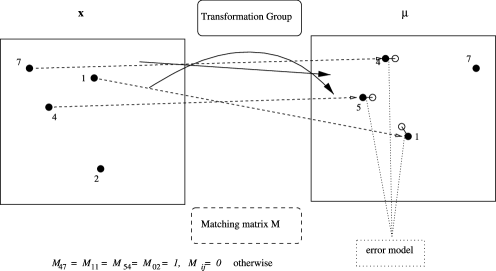
Figure 2: Illustration of the main ingredients of a statistical model. The labels of the two configurations of points ($x$ and $\mu$) can be considered as arbitrary. Some of the $x$ points are aligned to some of the $\mu$ points by a transformation (e.g., translation, rotation) which belongs to a specified group. An $0/1$ matrix $M$ indicates which points match, with unmatched points in $x$ (point 2 in the illustration) assigned to label “0,” and a specific error model assumed for the magnitude of the residual after alignment.

In Section 2 we introduce our statistical model and emphasize the group of affine transformations belonging to $\mathcal{G}$ which is relevant to our example. The appropriate matching matrix $M$ is estimated under various scenarios, including the use of a matrix $Q$ of prior probabilities, which is introduced to reflect the existence of the markers (labeled points)—an integral part of the specific problem. In Section 3 we outline likelihood based inference for $M$, and describe an EM algorithm. In Section 4 we adapt the prior matrix $Q$ when either a marker is missing or a marker is wrongly identified. Two real examples are studied in Section 5 related to renal cancer. In the first example, one marker is grossly misallocated and in the second example, some markers are missing. This procedure has great potential to automate preprocessing of the gels. We conclude with a discussion.

2 Statistical models

2.1 Transformations

Although the statistical model we later introduce can apply to various types of transformations, we focus on an affine transformation of the form $g(\mu)=\mu A^{\prime}+B^{\prime}$, where $A$ is a nonsingular $d\times d$ matrix and the $d\times 1$ vector, $b$, is present in every column of the $d\times(K+m)$ matrix $B$.

2.2 Matching matrix

To estimate the parameters of an appropriate transformation of $\mu$, we can introduce a correspondence system that will indicate whether a point in $\mu$ is associated with a point in $x$, that is, whether two points match across configurations. We can record the correspondence information in a $(K+m+1)\times(K+n)$ matching matrix, $M$, where

$$M_{ij}=\cases{1,&\quad$\mbox{for }i=0\mbox{ if }x_{j}\mbox{ does not have a matching point in }\mu,$\vspace*{2pt}\cr 1,&\quad$\mbox{for }i=1,\ldots,K+m\mbox{ if }x_{j}\mbox{ matches }\mu_{i},$\vspace*{2pt}\cr 0,&\quad$\mbox{otherwise}$}$$

for $j=1,\ldots,K+n$. Note that, for simplicity of notation, we use $M_{0j}\equiv M_{K+m+1,j}$, and similarly for other matrices. If $M_{0j}=1$, then $x_{j}$ does not have a matching point in $\mu$ and we say that $x_{j}$ is unmatched.

We consider one-to-one or many-to-one matches between points in $x$ and points in $\mu$. We refer to these as hard and soft matches, respectively. Soft matching can be useful in our application since a single protein can produce multiple spots on an image [Banks et al. (2000)].

Hard matches: The matching matrix, $M$, has the following constraints for the hard model:

$$\sum_{i=0}^{K+m}M_{ij}=1\qquad\mbox{for }j=1,\ldots,K+n$$ (1)

and

$$\sum_{j=1}^{K+n}M_{ij}\leq 1\qquad\mbox{for }i=1,\ldots,K+m.$$ (2)

So for $i_{1}\neq 0$, if $M_{i_{1}j_{1}}=1$, then $M_{i_{1}j_{2}}=M_{i_{2}j_{1}}=0$ for all $i_{1}\neq i_{2}$ and $j_{1}\neq j_{2}$. Note that there are no constraints on row $K+m+1$ in $M$ since each of the $K+n$ points in $x$ is free to remain unmatched. Figure 2 illustrates the case of hard matches in which the point $x_{2}$ is unmatched, so $M_{02}=1$.

Soft matches: For the soft model, the only constraint is stated in (1). That is, if $M_{i_{1}j_{1}}=1$, then $M_{i_{2}j_{1}}=0$ for all $i_{1}\neq i_{2}$, but $M_{i_{1}j_{2}}\in\{0,1\}$ for $j_{1}\neq j_{2}$. When assigning either hard or soft matches, (1) constrains a point in $x$ to be matched to a single point in $\mu$ or, alternatively, to remain unmatched.

2.3 Error distribution

Assuming the transformation parameters,$A$ and $b$, are known, we can apply a distribution to $x_{j}$ given the match $M_{ij}=1$. Given the transformation, we treat the elements of $x$ as conditionally independent with the following densities for $j=1,\ldots,K+n$:

$$p(x_{j}|M_{ij}=1)=\cases{\displaystyle\frac{1}{(2\pi\sigma^{2})^{d/2}}\exp\biggl{\{}-\frac{\|x_{j}-A\mu_{i}-b\|^{2}}{2\sigma^{2}}\biggr{\}},\vspace*{2pt}\cr\hskip 33.0pt\quad\mbox{for }i=1,\ldots,K+m,\vspace*{2pt}\cr\displaystyle\frac{1}{|\Omega|},\qquad\mbox{for }i=0,}$$ (3)

where $\Omega$ is some region in $\mathbb{R}^{d}$ containing all points in $x$.

To allow for the possibility of soft matching, we consider points in $x$ to be independent. As we have $K$ markers in each image, we have prior information about the matching across images. Next we introduce notation to deal with prior matching probabilities.

2.4 Prior matching matrix probabilities

Let $Q$ be a $(K+m+1)\times(K+n)$ matrix with elements $q_{ij}=p(M_{ij}=1)$. That is, for $j=1,\ldots,K+n$, $q_{ij}$ is the prior probability that $\mu_{i}$ is matched to $x_{j}$ for $i=1,\ldots,K+m$ and the prior probability that $x_{j}$ is unmatched for $i=0$. Again, for simplicity of notation, we use $q_{0j}$ in place of $q_{K+m+1,j}$. Note that $\sum_{i=0}^{K+m}q_{ij}=1\mbox{ for }j=1,\ldots,K+n$. We have prior knowledge that corresponding markers, $\mu_{j}$ and $x_{j}$ for $j=1,\ldots,K$, should match. We propose a structure to determine the $q_{ij}$, which accounts for the possibility of error when allocating markers within a warped image and does not force corresponding markers to match. In what follows, it will be helpful to note that the matrix $Q$ can be partitioned into submatrices of size (rows $\times$ columns) as follows:

$$Q\bigl{(}(1+K+m)\times(K+n)\bigr{)}$$

$$\qquad=\pmatrix{Q^{(0)}(1\times K)&\mid&\vspace*{2pt}\cr---------&\mid\vspace*{2pt}\cr&\mid&Q^{(2)}\bigl{(}(1+K+m)\times n\bigr{)}\vspace*{2pt}\cr Q^{(1)}\bigl{(}(K+m)\times K\bigr{)}&\mid\vspace*{2pt}\cr&\mid&}.$$

Markers in $x$: We know that $\mu_{j}$ are the coordinates for marker $j$ in $\mu$, $j=1,\ldots,K$. Let $\gamma_{j}$ be the index of the true marker $j$ in $\mu$. If $\gamma_{j}=j$, then the marker $j$ has been correctly identified. We set the prior probability of a point $\mu_{i}$ being the true marker $j$, $q_{ij}$, to be a function of the distance between $\mu_{i}$ and $\mu_{j}$ so that $Q^{(1)}$ has elements

$$q_{ij}=p(\gamma_{j}=i)=f(d_{ij})\qquad\mbox{for }i=1,\ldots,K+m,j=1,\ldots,K,$$ (4)

where $d_{ij}$ is the Euclidean distance between $\mu_{i}$ and $\mu_{j}$ and choices for $f$ are discussed later.

Next we consider the possibility that a marker within $x$ does not have a corresponding point in $\mu$. Recall that $x_{j}$ are the coordinates for marker $j$ in $x$, $j=1,\ldots,K$. To allow for the possibility that $x_{j}$ remains unmatched, we set the prior probability of $M_{0j}=1$ to be uniform so that $Q^{(0)}$ has elements

$$q_{0j}=p(\gamma_{j}=0)=\frac{1}{|\Omega|}\qquad\mbox{for }j=1,\ldots,K,$$ (5)

where $\Omega$ is given as in (3).

Nonmarkers in $x$: To allow for matching of the nonmarker points, we can set the elements of $Q^{(2)}$ as

$$q_{ij}=\frac{1}{K+m+1},\qquad i=0,\ldots,K+m,j=K+1,\ldots,K+n.$$ (6)

So the prior matching probability of a nonmarker $x_{j}$ is uniform.

As an example, we suppose that in Figure 2 only point 1 has been identified as a marker in both $x$ and $\mu$, then we might have $q_{01}=0.01$ ($=1/|\Omega|$, say), $q_{11}=0.89$, $q_{41}=0.01$, $q_{51}=0.09$, $q_{71}=0.00$ (based on the interpoint distances within $\mu$) and $q_{ij}=1/8$ for the other points shown (taking $m=6$ in this example).

For ease of reference, the ingredients of the statistical model, together with possible variations, are listed in Table 1.

Table 1: Main ingredients of the statistical model used for matching of partially labeled configurations of points. Section numbers [e.g., (3.1)] are used to sign-post further details or discussion

Component of model	Variants	Examples
Configurations $x$ and $\mu$	Unlabeled (Section 1.2)
	Partially labeled	Markers (Section 1.1)
Transformation group	Rigid-body (Section 2.1)
	Affine (Section 3.1)
	Nonlinear (Section 6)
Matching matrix, $M$	Hard (Section 6)	One-to-one
	Soft	Many-to-one (Section 6)
		Many-to-many (Section 6)
Prior matrix, $Q$,
with $Q_{ij}=P(M_{ij}=1)$
which depends on
– markers (Section 4)	Function of distance (Section 3.3.1)
– nonmarkers
Error distribution	Isotropic (Section 2.3)
	Nonlinear (Section 6)

3 EM algorithms and inference

3.1 EM algorithm

We use an EM algorithm [McLachlan and Krishnan (2008)] to estimate the transformation parameters, $A$ and $b$, that will superimpose $\mu$ onto $x$. Throughout this section we assume that $\sigma^{2}$ has been assigned (see Section 3.3.3). In the E-step we calculate the posterior probability that $\mu_{i}$ matches $x_{j}$, that is, the posterior probability that $M_{ij}=1$. In the M-step the posterior probabilities are input into the expected likelihood of observing $M$, given the data, $x$. This enables us to estimate the transformation parameters, $A$ and $b$.

E-step: We calculate the posterior probability of $\mu_{i}$ matching $x_{j}$, given the data, using Bayes’ theorem:

$$p(M_{ij}=1|x_{j})=\frac{p(x_{j}|M_{ij}=1)p(M_{ij}=1)}{p(x_{j})},$$ (7)

where $p(x_{j}|M_{ij}=1)$ is calculated using (3), and $q_{ij}=p(M_{ij}=1)$ is calculated using (4)–(6). The denominator of (7) is given by $\sum_{i=0}^{K+m}p(x_{j}|M_{ij}=1)\times p(M_{ij}=1)$.

M-step: Starting from the multinomial form [McLachlan and Krishnan (2008), page 15]

$$l(M|x)=\sum_{i=0}^{K+m}\sum_{j=1}^{K+n}M_{ij}\log p(x_{j}),$$

we substitute $p_{ji}$ for $M_{ij}$ and $q_{ij}p(x_{j}|M_{ij}=1)$ for $p(x_{j})$to obtain the expected log-likelihood of the matching matrix, $M$, given the data, $x$:

$$\mathsf{E}[l(M|x)]=\sum_{i=0}^{K+m}\sum_{j=1}^{K+n}p_{ji}[\log q_{ij}+\log p(x_{j}|M_{ij}=1)].$$ (8)

Here, we suppress the dependence on the parameters $A$ and $b$.

Both the prior probabilities stored in $Q$ and the conditional distribution of $x_{j}$ being unmatched are independent of $A$ and $b$, so, using (8), we estimate the transformation parameters that maximize

$$\sum_{i=1}^{K+m}\sum_{j=1}^{K+n}p_{ji}\log p(x_{j}|M_{ij}=1)$$

$$\qquad=\sum_{i=1}^{K+m}\sum_{j=1}^{K+n}p_{ji}\biggl{[}-\frac{\|x_{j}-A\mu_{i}-b\|^{2}}{2\sigma^{2}}-\frac{d}{2}\log(2\pi\sigma^{2})\biggr{]}.$$

Note that the final term is a constant, given that $\sigma$ is assumed known. Removing further terms independent of $A$ and $b$, we want to estimate the transformation parameters that minimize

$$\sum_{i=1}^{K+m}\sum_{j=1}^{K+n}p_{ji}\|x_{j}-A\mu_{i}-b\|^{2}.$$

Ignoring the terms independent of $b$, and noting that $\partial a^{\prime}x/\partial x=a$ and $\partial x^{\prime}x/\partial x=2x$, the maximum likelihood estimates [Walker (2000)] are

$$\hat{b}=\frac{\sum_{i=1}^{K+m}\sum_{j=1}^{K+n}p_{ji}(x_{j}-A\mu_{i})}{\sum_{i=1}^{K+m}\sum_{j=1}^{K+n}p_{ji}}$$ (9)

and

$$\hat{A} = \Biggl{[}\sum_{i=1}^{K+m}\sum_{j=1}^{K+n}p_{ji}(x_{j}-\bar{x})(\mu_{i}-\bar{\mu})^{\prime}\Biggr{]}$$

$${}\times\Biggl{[}\sum_{i=1}^{K+m}\sum_{j=1}^{K+n}p_{ji}(\mu_{i}-\bar{\mu})(\mu_{i}-\bar{\mu})^{\prime}\Biggr{]}^{-1}.$$

The algorithm alternates between the E-step and the M-step. At each iteration, the transformation parameters are updated in the M-step to $A^{(r+1)}=\hat{A}^{(r)}$ and $b^{(r+1)}=\hat{b}^{(r)}$, before substitution into the E-step for the next iteration.

We assign convergence to be when $r$ is such that

$$\frac{1}{(K+m+1)(K+n)}\sum_{i=0}^{K+m}\sum_{j=1}^{K+n}\bigl{[}p_{ji}^{(r+1)}-p_{ji}^{(r)}\bigr{]}^{2}\leq 10^{-l},$$ (11)

where $l$ is chosen and the posterior probability of $\mu_{i}$ matching $x_{j}$ at the $r$th and $(r+1)$st iteration is denoted by $p_{ji}^{(r)}$ and $p_{ji}^{(r+1)}$, respectively, for $i=0,\ldots,K+m$ and $j=1,\ldots,K+n$.

3.2 Inference for $M$

Let $P$ be the $(K+n)\times(K+m+1)$ matrix containing the final posterior matching probabilities. Let $\hat{A}$ and $\hat{b}$ be the final estimates of the transformation parameters obtained from the EM algorithm.

An obvious route to estimate the matching matrix, $M$, is to use the posterior matching probabilities, but this will not yield a one-to-one outcome. For one-to-one matches we need to satisfy the constraints in (1) and (2). Given the transformation, the conditional log-likelihood of $M$ is $\sum_{i=0}^{K+m}\sum_{j=1}^{K+n}M_{ij}\log P_{ji}$. We find $M$ that maximizes this log-likelihood by mixed integer linear programming. In our implementation we imputted the $2K+m+n$ constraints into lp_solve [Berkelaar (2008)], which then yields the estimated one-to-one matching matrix, $\hat{M}$. We can summarize the steps as follows.

1. [(iii)]

2. Assign $q_{ij}$ using (4), (5) and (6) for $i=0,\ldots,K+m$ and $j=1,\ldots,K+n$.

3. Find initial estimates of the transformation parameters, $A^{(0)}$ and $b^{(0)}$, and assign the variance, $\sigma^{2}$. Possible choices are discussed in the following subsection.

4. Run the EM algorithm to get the updated estimates, $p_{ji}^{(1)}$, $A^{(1)}$ and $b^{(1)}$, using (7), (3.1) and (9), respectively.

5. Repeat step 3 to find the updated estimates, $p_{ji}^{(r+1)}$, $A^{(r+1)}$ and $b^{(r+1)}$, until convergence [defined in (11)] is reached. Let the final posterior matching probabilities be stored in the $(K+n)\times(K+m+1)$ matrix $P$ and the final estimated transformation parameters be denoted by $\hat{A}$ and $\hat{b}$.

6. One-to-one matches are obtained using the hardening algorithm described above.

7. Treating the matches within the inferred matching matrix, $\hat{M}$, as known, we can update the transformation parameters using Procrustes methodology [Dryden and Mardia (1998)] to calculate the final estimates, $\hskip 3.0pt\hat{\hat{A}}$ and $\hskip 1.0pt\hat{\hat{b}}$.

3.3 Assigning the function and parameters within the EM algorithm

We need to assign the function $f$ stated in (4), as well as starting values for the transformation parameters denoted by $A^{(0)}$ and $b^{(0)}$, and a variance $\sigma^{2}$. We look at each assignment separately.

3.3.1 Distance function

As before, $\mu_{j}$ contains the allocated marker coordinates for marker $j$ in $\mu$, $j=1,\ldots,K$, and $\gamma_{j}$ is the index of the true marker $j$ in $\mu$. Let $\bar{d}_{ij}$ denote the expected distance between a point $\mu_{i}$ and $\mu_{j}$ for $i=1,\ldots,K+m$. Due to the freedom for a gel to warp, in reality the distance between $\mu_{i}$ and $\mu_{j}$ in an image is $d_{ij}=\bar{d}_{ij}+\varepsilon$, where $\varepsilon$ denotes some error.

Our choice of the function, $f$, in (4), considers all points in $\mu$ as possible true markers. We adopt a multivariate normal distribution for $\varepsilon$, which gives

$$q_{ij}=p(\gamma_{j}=i)\propto\exp\biggl{\{}-\frac{\|\mu_{i}-\mu_{j}\|^{2}}{2\sigma_{*}^{2}}\biggr{\}},$$ (12)

for $i=1,\ldots,K+m$, where $\sigma_{*}^{2}$ is the variance between two points in $\mu$ (assuming independence across dimensions). So the probability that $\mu_{i}$ is the true marker $j$ will decrease the further it is from $\mu_{j}$.

3.3.2 Starting values for transformation parameters

As we have prior knowledge of allocated corresponding markers in both $\mu$ and $x$, it is sensible that $A^{(0)}$ and $b^{(0)}$ are set as the transformation parameters necessary to best superimpose corresponding markers. Dryden and Mardia (1998) show how these parameters can be estimated from the matrix,

$$R=(\mu_{*}^{\prime}\mu_{*})^{-1}\mu_{*}^{\prime}x^{(m)},$$ (13)

where $\mu_{*}$ is the $K\times(d+1)$ matrix $\mu_{*}=(\underline{1}_{K},\mu^{(m)})$ and $\underline{1}_{K}$ is a vector of ones of length $K$. The $K\times d$ matrices, $\mu^{(m)}$ and $x^{(m)}$, contain only the marker coordinates for $\mu$ and $x$, respectively.

The first column in $R^{\prime}$ contains $b^{(0)}$ and the second two columns in $R^{\prime}$ contain the $d\times d$ matrix $A^{(0)}$.

3.3.3 Starting values for the variance between images

We can estimate the variance $\sigma^{2}$ by considering the mean squared distance between corresponding markers in $\mu$ and $x$ after an affine transformation has been applied to superimpose them. That is, set

$$\hat{\sigma}^{2}=\frac{1}{\nu}\sum_{j=1}^{K}\bigl{\|}x_{j}-A^{(0)}\mu_{j}-b^{(0)}\bigr{\|}^{2},$$ (14)

where $\nu=dK-d^{2}-d$ and denotes the degrees of freedom. Here $dK$ is the number of error terms in the $d$ components of the $K$ markers. This number is reduced in $\nu$ to accommodate the estimates of $A^{(0)}$ and $b^{(0)}$.

4 Grossly misallocated or missing markers

This section describes further refinements to the above Composite Algorithm, which is highly dependent on the transformation parameters input as starting values, $A^{(0)}$ and $b^{(0)}$. We have previously stated that the affine transformation necessary to superimpose corresponding markers in $\mu$ and $x$ will provide sensible starting values for the transformation parameters within the EM algorithm. However, this would not be the case if gross misallocations occur. The number of missing or grossly misidentified markers are dependent on the quality of the equipment and the expert that creates the images.

First, we provide a method that will highlight grossly misallocated markers across images. Highlighted markers can then be automatically removed or corrected before they are used within the EM algorithm to estimate transformation starting values. Then, in Section 4.2 we deal with the case where some markers are missing from one of the images.

4.1 Grossly misallocated markers

Gross misallocations of a marker may occur through human error when inputting marker labels into data spreadsheets. Dryden and Walker (1999) consider procedures based on S estimators, least median of squares and least quartile difference estimators that are highly resistant to outlier points. The RANSAC algorithm [Fischler and Bolles (1981)] uses a similar robust strategy. Here we describe how we can use the EM algorithm previously described.

Here we provide a method that will highlight grossly misallocated markers across images. Highlighted markers can then be automatically removed or corrected before they are used within the EM algorithm to estimate transformation starting values.

Let $\mu^{(m)}$ and $x^{(m)}$ be $K\times d$ coordinate matrices where $\mu_{j}$ and $x_{j}$ contain the coordinates of marker $j$ in $\mu$ and $x$, respectively, for $j=1,\ldots,K$. Here we consider the prior matching probabilities to be independent of the distance between a possible marker and the allocated marker so that

$$q_{ij}=\cases{p_{M},&\quad$\mbox{for }i=j,$\vspace*{2pt}\cr\displaystyle\frac{1-p_{M}}{K},&\quad$\mbox{for }i\neq j,$}$$ (15)

where $p_{M}$ denotes the probability that the allocated marker $\mu_{j}$ truly corresponds to the allocated marker $x_{j}$.

We input $\mu^{(m)}$ and $x^{(m)}$ into steps (i)–(v) of the composite algorithm to estimate the one-to-one matching matrix $\hat{M}$, replacing (4) and (5) with (15) in stage (i). We use (13) to estimate the starting transformation values, $A^{(0)}$ and $b^{(0)}$. Note that the starting transformation will be distorted by the presence of grossly misallocated markers. There are four possible outcomes for $k=1,\ldots,K$:

• The allocated corresponding markers $\mu_{k}$ and $x_{k}$ are matched if $\hat{M}_{kk}=1$. We include both $\mu_{k}$ and $x_{k}$ in further analyses.

• The marker $x_{k}$ remains unmatched if $\hat{M}_{0k}=1$. We exclude both $\mu_{k}$ and $x_{k}$ from further analyses.

• No point in $x^{(m)}$ is matched to the marker $\mu_{k}$ if $\hat{M}_{kj}=0$, for all $j=1,\ldots,K$. We exclude both $\mu_{k}$ and $x_{k}$ from further analyses.

• The marker $\mu_{k_{1}}$ is matched to an allocated noncorresponding marker $x_{k_{2}}$ if $\hat{M}_{k_{1}k_{2}}=1$, for $k_{1}\neq k_{2}$. We exclude $\mu_{k_{1}}$, $\mu_{k_{2}}$, $x_{k_{1}}$ and $x_{k_{2}}$ from further analyses.

See Section 5.1 for an illustration.

4.2 Missing markers

It is possible that all $K$ markers are not successfully located in both $\mu$ and $x$. For example, only 10 out of the possible $K=12$ markers were located in the image displayed in Figure 1.

There are four possible cases we must consider for Marker $k=1,\ldots,K$: (a) located in both $\mu$ and $x$; (b) located in $\mu$ alone; (c) located in $x$ alone; and (d) not located in either $\mu$ or $x$. We first introduce notation to allow for the possibility of missing markers.

Let $K_{\mu}$ and $K_{x}$ be the total number of markers located in $\mu$ and $x$, respectively. As previously noted, let $\mu$ be the $(K+m)\times d$ coordinate matrix and $x$ be the $(K+n)\times d$ coordinate matrix.

If marker $k$ is located in $\mu$, then $\mu_{k}$ contains the coordinates of marker $k$ in $\mu$. If marker $k$ is not located in $\mu$, then $\mu_{k}=\varnothing$. Similarly, if marker $k$ is located in $x$, then $x_{k}$ contains the coordinates of marker $k$ in $x$, for $k=1,\ldots,K$. If marker $k$ is not located in $x$, then $x_{k}=\varnothing$.

As previously stated, $Q$ is the $(K+m+1)\times(K+n)$ matrix containing the prior matching probabilities for points in $x$. We define $Q$ by allowing for the possibility that an allocated marker $k$ is not the true marker $k$, for $k=1,\ldots,K$.

Markers in $x$: corresponding to each of the above cases we have: [(a)]

If $\mu_{j}\neq\varnothing$ and $x_{j}\neq\varnothing$, we assign $q_{ij}$ as previously stated in (4) and (5) for $i=0,\ldots,K+m$.

If $\mu_{j}\neq\varnothing$ and $x_{j}=\varnothing$, we treat $\mu_{j}$ as a nonmarker.

If $\mu_{j}=\varnothing$ and $x_{j}\neq\varnothing$, we treat $x_{j}$ as a nonmarker.

If $\mu_{j}=\varnothing$ and $x_{j}=\varnothing$, we set $q_{ij}=q_{jk}=\varnothing$ for all $i$ and $k$.

Nonmarkers in $x$: The prior matching probability of a nonmarker, $x_{j}$, is again set to be uniform over all matching possibilities so that, for $i=0,\ldots,K+m$ and $j=K+1,\ldots,K+n$,

$$q_{ij}=\frac{1}{K_{\mu}+m+1}.$$ (16)

In case 3, when $\mu_{j}=\varnothing$ and $x_{j}\neq\varnothing$ for $j=1,\ldots,K$, we treat $x_{j}$ as a nonmarker and use (16) to calculate $q_{ij}$ for $i=0,\ldots,K+m$.

Note that $\mu$ contains $K_{\mu}$ markers and $m$ nonmarkers. There are only $K_{\mu}+m+1$ matching possibilities for a point in $x$, thus producing the denominator in (16). See Section 5.2 for an illustration.

5 Examples

Our full data set—see Supplementary Material [Mardia, Petty and Taylor (2012)]—was collected to represent eight subjects, under two different conditions, treated with two possible treatments.

A replicate image was also produced for each subject-treatment specific case. A typical Western Blot is shown in Figure 1, which is approximately of size $280\times 220$. In this paper we illustrate the methods on two pairs of images: in the first example, robustness to gross misidentification is explored, and the second example deals with missing markers.

5.1 Grossly misallocated marker

Let $\mu$ and $x$ represent the coordinate sets on Western Blots of a renal cancer cell line cultured under either normoxic or hypoxic conditions. The proteins are then extracted and probed with either patient sera or control sera in a Western Blot to produce the images generated. All $K=12$ markers were located in both images.

We input the corresponding markers for $\mu$ and $x$ into steps (i)–(v) of the composite algorithm (see Section 3.2) to estimate the one-to-one matching matrix, $\hat{M}$, found when superimposing $\mu^{(m)}$ onto $x^{(m)}$. That is, we transform the appropriate markers in $\mu$ onto the corresponding markers in $x$. Using only the markers, we estimate the variance in (3) as $\hat{\sigma}^{2}=4.5^{2}$ and set the prior matching probability in (15) as $p_{M}=0.99$. The starting values for the transformation parameters, $A^{(0)}$ and $b^{(0)}$, are found using (13). We use the final posterior probabilities, $P$, to estimate $M$. Marker $1$ remains unmatched in both images.

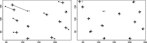
Figure 3: Initial transformation, before (left) and after (right) marker $1$ is removed as a marker from both images.

Figure 3 shows the initial transformation of $\mu$ onto $x$ before and after marker $1$ is removed as a marker (though still displayed) in both images. In this example, the RMSD between the $12$ marker pairs before the removal is $19.44$. The RMSD between the remaining $11$ marker pairs after the removal is $2.96$.

Following these discoveries, we were told that marker $1$ was incorrectly labeled as spotID 136 when it should have been spotID 153, that is, the methodology was able to highlight a misidentified marker.

5.2 Missing markers

In this example we display the matches made when comparing two replicate specimens, representing a cell line cultured under either normoxic conditions, with proteins extracted and probed with control sera. All $12$ markers were located in $\mu$. Markers $9$ and $10$ were missing in $x$, so these were treated as nonmarkers in $\mu$ and we set $K=10$.

We input the images into steps (i)–(v) of the composite algorithm. The starting values for the transformation parameters, $A^{(0)}$ and $b^{(0)}$, are found using (13). We estimate the variance in (3), $\sigma^{2}$, using (14) with denominator $\nu$. Finally, we set $\hat{\sigma}_{*}^{2}=\hat{\sigma}^{2}$ in (12). The estimated transformation parameters are

$$\hat{A}=\pmatrix{0.980&-0.047\vspace*{2pt}\cr 0.002&1.006}$$

and $\hat{b}=(-1.72,10.78)^{\prime}$. We display the matches made in Figure 4 after the final transformation of $\mu$ onto $x$.

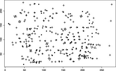
Figure 4: Final transformation of $\mu$ onto $x$ and the matches made. Points in $x$ ($\bullet$), points in transformed $\mu$ ($+$), markers in $x$ ($\triangledown$) and markers in $\mu$ ($\triangle$). The 107 matched points across images are joined by a line.

6 Discussion

Many EM algorithms are known to converge only to a local solution, and this will also apply to the methods considered here. However, the availability of the markers which provide partial information will usually ensure good starting values, so this will not be a problem in our application.

Note that it would be possible to adapt the model so that $\sigma$ could be allowed to vary according to the distance of the point to the edge of the image, which could be used to deal with minor nonlinear deformations. More generally, it should also be possible to adapt our methods to deal with more general transformations, for example, using thin-plate splines [Chui and Rangarajan (2003)].

There are situations when clusters occur within a gel which makes it difficult to correctly identify a marker within a cluster of points. We can allow for the increased likelihood that a marker $\mu_{j},j=1,\ldots,K$, is misallocated if it exists within a cluster of other points, by using an adaptive choice of $f$ in the prior (4):

$$q_{ij}=p(\gamma_{j}=i)\propto\cases{\displaystyle\frac{1}{C_{j}},&\quad$\mbox{if }d_{ij}\leq\varepsilon,$\vspace*{2pt}\cr 0,&\quad$\mbox{if }d_{ij}>\varepsilon,$}$$

where $d_{ij}$ is the Euclidean distance and $C_{j}$ is the number of points in $\mu$ that are within a distance of $\varepsilon$ from $\mu_{j}$, that is,

$$C_{j}=\sum_{i=1}^{K+m}I[d_{ij}\leq\varepsilon],$$

where $I[d_{ij}\leq\varepsilon]=1$ if $d_{ij}\leq\varepsilon$, ($0$ otherwise) for $i=1,\ldots,K+m$.

A further adaptation of the model, which could be useful in Western Blots, would be to incorporate in the priors a measure associated with the grey-scale intensity of the located points in the image [Rohr, Cathier and Wörz (2004)]. Approaches for this, as well as further models for the background noise, are considered in Petty (2009).

Our composite algorithm ensures one-to-one matches, but there are circumstances in which many-to-one or many-to-many matches can be considered. These can be useful when comparing protein images since multiple forms of an individual protein can often be visualized [Banks et al. (2000)]. That is, a single protein can produce multiple spots on an image.

It should be noted that our model is asymmetric in $\mu$ and $x$. This is not uncommon; for example, the full Procrustes error is not symmetrical [see Dryden and Mardia (1998)]. Also, the standard RMSD used by bioinformatricians is again not a symmetrical measure. However, there are symmetrical unlabeled shape analyses; see Green and Mardia (2006), for example. However, this method has not been developed for affine transformations and warping as required here. There is also a nonprobabilistic method of Rangarajan, Chui and Bookstein (1997) for similarity shape, but again the extension of the method to affine transformations and warping requires further work; see Kent, Mardia and Taylor (2010b) for a statistical framework. For the data considered here, we have verified that reversing the role of $\mu$ and $x$ does not change the broad conclusions.

Finally, we note that the methods described in this paper could have applications in other situations in which there are unlabeled points, some of which—possibly with error—have been manually identified. Thus, the method could be used in the preparation of ground truth for training an object recognition system or a pose estimation system; for example, see the survey of Murphy-Chutorian and Trivedi (2008).

References

- Banks et al. (2000) {barticle}[pbm] \bauthor\bsnmBanks, \bfnmR. E.\binitsR. E., \bauthor\bsnmDunn, \bfnmM. J.\binitsM. J., \bauthor\bsnmHochstrasser, \bfnmD. F.\binitsD. F., \bauthor\bsnmSanchez, \bfnmJ. C.\binitsJ. C., \bauthor\bsnmBlackstock, \bfnmW.\binitsW., \bauthor\bsnmPappin, \bfnmD. J.\binitsD. J. and \bauthor\bsnmSelby, \bfnmP. J.\binitsP. J. (\byear2000). \btitleProteomics: New perspectives, new biomedical opportunities. \bjournalLancet \bvolume356 \bpages1749–1756. \biddoi=10.1016/S0140-6736(00)03214-1, issn=0140-6736, pii=S0140-6736(00)03214-1, pmid=11095271 \bptokimsref \endbibitem
- Berkelaar (2008) {bmisc}[auto:STB—2012/04/05—08:30:55] \bauthor\bsnmBerkelaar, \bfnmM.\binitsM. (\byear2008). \bhowpublishedInterface to lp_solve v. 5.5 to solve linear/integer programs, R package. \bptokimsref \endbibitem
- Besl and McKay (1992) {barticle}[auto:STB—2012/04/05—08:30:55] \bauthor\bsnmBesl, \bfnmP. J.\binitsP. J. and \bauthor\bsnmMcKay, \bfnmN. D.\binitsN. D. (\byear1992). \btitleA method for registration of 3-D shapes. \bjournalIEE Trans. PAMI \bvolume14 \bpages239–256. \bptokimsref \endbibitem
- Chen (2011) {barticle}[mr] \bauthor\bsnmChen, \bfnmPengwen\binitsP. (\byear2011). \btitleA novel kernel correlation model with the correspondence estimation. \bjournalJ. Math. Imaging Vision \bvolume39 \bpages100–120. \biddoi=10.1007/s10851-010-0230-6, issn=0924-9907, mr=2788514 \bptokimsref \endbibitem
- Chui and Rangarajan (2003) {barticle}[auto:STB—2012/04/05—08:30:55] \bauthor\bsnmChui, \bfnmH.\binitsH. and \bauthor\bsnmRangarajan, \bfnmA.\binitsA. (\byear2003). \btitleA new point matching algorithm for non-rigid registration. \bjournalComputer Vision and Understanding \bvolume89 \bpages114–141. \bptokimsref \endbibitem
- Czogiel, Dryden and Brignell (2011) {bmisc}[auto:STB—2012/04/05—08:30:55] \bauthor\bsnmCzogiel, \bfnmI.\binitsI., \bauthor\bsnmDryden, \bfnmI. L.\binitsI. L. and \bauthor\bsnmBrignell, \bfnmC. J.\binitsC. J. (\byear2011). \bhowpublishedBayesian matching of unlabeled marked point sets using random feilds, with an application to molecular alignment. Ann. Appl. Stat. 5 2603–2629. \bptokimsref \endbibitem
- Dryden, Hirst and Melville (2007) {barticle}[mr] \bauthor\bsnmDryden, \bfnmIan L.\binitsI. L., \bauthor\bsnmHirst, \bfnmJonathan D.\binitsJ. D. and \bauthor\bsnmMelville, \bfnmJames L.\binitsJ. L. (\byear2007). \btitleStatistical analysis of unlabeled point sets: Comparing molecules in chemoinformatics. \bjournalBiometrics \bvolume63 \bpages237–251, 315. \biddoi=10.1111/j.1541-0420.2006.00622.x, issn=0006-341X, mr=2345594 \bptokimsref \endbibitem
- Dryden and Mardia (1998) {bbook}[mr] \bauthor\bsnmDryden, \bfnmI. L.\binitsI. L. and \bauthor\bsnmMardia, \bfnmK. V.\binitsK. V. (\byear1998). \btitleStatistical Shape Analysis. \bpublisherWiley, \baddressChichester. \bidmr=1646114 \bptokimsref \endbibitem
- Dryden and Walker (1999) {barticle}[auto:STB—2012/04/05—08:30:55] \bauthor\bsnmDryden, \bfnmI. L.\binitsI. L. and \bauthor\bsnmWalker, \bfnmG.\binitsG. (\byear1999). \btitleHighly resistance regression and object matching. \bjournalBiometrics \bvolume55 \bpages820–825. \bptokimsref \endbibitem
- Fischler and Bolles (1981) {barticle}[mr] \bauthor\bsnmFischler, \bfnmMartin A.\binitsM. A. and \bauthor\bsnmBolles, \bfnmRobert C.\binitsR. C. (\byear1981). \btitleRandom sample consensus: A paradigm for model fitting with applications to image analysis and automated cartography. \bjournalComm. ACM \bvolume24 \bpages381–395. \biddoi=10.1145/358669.358692, issn=0001-0782, mr=0618158 \bptokimsref \endbibitem
- Forgber et al. (2009) {barticle}[auto:STB—2012/04/05—08:30:55] \bauthor\bsnmForgber, \bfnmM.\binitsM., \bauthor\bsnmGellrich, \bfnmS.\binitsS., \bauthor\bsnmSharav, \bfnmT.\binitsT., \bauthor\bsnmSterry, \bfnmW.\binitsW. and \bauthor\bsnmWalden, \bfnmP.\binitsP. (\byear2009). \btitleProteome-based analysis of serologically defined tumor-associated antigens in cutaneous lymphona. \bjournalPloS ONE \bvolume4 \bpagese8376. \bptokimsref \endbibitem
- Glaunes, Trouvé and Younes (2004) {barticle}[auto:STB—2012/04/05—08:30:55] \bauthor\bsnmGlaunes, \bfnmJ.\binitsJ., \bauthor\bsnmTrouvé, \bfnmA.\binitsA. and \bauthor\bsnmYounes, \bfnmL.\binitsL. (\byear2004). \btitleDiffeomorphic matching of mistributions: A new approach for unlabelled point-sets and sub-manifolds matching. \bjournalCVPR \bvolume2 \bpages712–718. \bptokimsref \endbibitem
- Green and Mardia (2006) {barticle}[mr] \bauthor\bsnmGreen, \bfnmPeter J.\binitsP. J. and \bauthor\bsnmMardia, \bfnmKanti V.\binitsK. V. (\byear2006). \btitleBayesian alignment using hierarchical models, with applications in protein bioinformatics. \bjournalBiometrika \bvolume93 \bpages235–254. \biddoi=10.1093/biomet/93.2.235, issn=0006-3444, mr=2278080 \bptokimsref \endbibitem
- Green et al. (2010) {bincollection}[mr] \bauthor\bsnmGreen, \bfnmPeter J.\binitsP. J., \bauthor\bsnmMardia, \bfnmKanti V.\binitsK. V., \bauthor\bsnmNyirongo, \bfnmVysaul B.\binitsV. B. and \bauthor\bsnmRuffieux, \bfnmYann\binitsY. (\byear2010). \btitleBayesian modelling for matching and alignment of biomolecules. In \bbooktitleThe Oxford Handbook of Applied Bayesian Analysis \bpages27–50. \bpublisherOxford Univ. Press, \baddressOxford. \bidmr=2790338 \bptokimsref \endbibitem
- Kent, Mardia and Taylor (2010a) {bmisc}[auto:STB—2012/04/05—08:30:55] \bauthor\bsnmKent, \bfnmJ. T.\binitsJ. T., \bauthor\bsnmMardia, \bfnmK. V.\binitsK. V. and \bauthor\bsnmTaylor, \bfnmC. C.\binitsC. C. (\byear2010a). \bhowpublishedMatching unlabelled configurations and protein bioinformatics. Research Report STAT10-01. Univ. Leeds, Leeds, UK. \bptokimsref \endbibitem
- Kent, Mardia and Taylor (2010b) {bmisc}[auto:STB—2012/04/05—08:30:55] \bauthor\bsnmKent, \bfnmJ. T.\binitsJ. T., \bauthor\bsnmMardia, \bfnmK. V.\binitsK. V. and \bauthor\bsnmTaylor, \bfnmC. C.\binitsC. C. (\byear2010b). \bhowpublishedAn EM interpretation of the Softassign algorithm for alignment problems. In LASR10—High-throughput sequencing, proteins and statistics (A. Gusnanto, K. V. Mardia, C. J. Fallaize and J. Voss, eds.) 29–32. Dept. Statistics, Univ. Leeds, Leeds, UK. \bptokimsref \endbibitem
- Mardia, Petty and Taylor (2012) {bmisc}[auto:STB—2012/04/05—08:30:55] \bauthor\bsnmMardia, \bfnmKanti V.\binitsK. V., \bauthor\bsnmPetty, \bfnmEmma M.\binitsE. M. and \bauthor\bsnmTaylor, \bfnmCharles C.\binitsC. C. (\byear2012). \bhowpublishedSupplement to “Matching markers and unlabeled configurations in protein gels.” DOI:10.1214/ 12-AOAS544SUPP. \bptokimsref \endbibitem
- McLachlan and Krishnan (2008) {bbook}[mr] \bauthor\bsnmMcLachlan, \bfnmGeoffrey J.\binitsG. J. and \bauthor\bsnmKrishnan, \bfnmThriyambakam\binitsT. (\byear2008). \btitleThe EM Algorithm and Extensions, \bedition2nd ed. \bpublisherWiley, \baddressHoboken, NJ. \biddoi=10.1002/9780470191613, mr=2392878 \bptokimsref \endbibitem
- Murphy-Chutorian and Trivedi (2008) {barticle}[auto:STB—2012/04/05—08:30:55] \bauthor\bsnmMurphy-Chutorian, \bfnmE.\binitsE. and \bauthor\bsnmTrivedi, \bfnmM. M.\binitsM. M. (\byear2008). \btitleHead pose estimation in computer vision: A survey. \bjournalIEEE Transactions on Pattern Analysis and Machine Intelligence \bvolume31 \bpages607–626. \bptokimsref \endbibitem
- Petty (2009) {bmisc}[auto:STB—2012/04/05—08:30:55] \bauthor\bsnmPetty, \bfnmE. M.\binitsE. M. (\byear2009). \bhowpublishedShape analysis in bioinformatics. Ph.D. thesis, Univ. Leeds, Leeds, UK. \bptokimsref \endbibitem
- Rangarajan, Chui and Bookstein (1997) {bincollection}[auto:STB—2012/04/05—08:30:55] \bauthor\bsnmRangarajan, \bfnmA.\binitsA., \bauthor\bsnmChui, \bfnmH.\binitsH. and \bauthor\bsnmBookstein, \bfnmF. L.\binitsF. L. (\byear1997). \btitleThe Softassign Procrustes matching algorithm. In \bbooktitleInformation Processing in Medical Imaging 15th International Conference, IPMI’97 Poultney \bpages29–42. \bpublisherSpringer, \baddressNew York. \bptokimsref \endbibitem
- Rohr, Cathier and Wörz (2004) {barticle}[auto:STB—2012/04/05—08:30:55] \bauthor\bsnmRohr, \bfnmK.\binitsK., \bauthor\bsnmCathier, \bfnmP.\binitsP. and \bauthor\bsnmWörz, \bfnmS.\binitsS. (\byear2004). \btitleElastic registration of electrophoresis images using intensity information and point landmarks. \bjournalPattern Recognition \bvolume37 \bpages1035–1048. \bptokimsref \endbibitem
- Taylor, Mardia and Kent (2003) {bmisc}[auto:STB—2012/04/05—08:30:55] \bauthor\bsnmTaylor, \bfnmC. C.\binitsC. C., \bauthor\bsnmMardia, \bfnmK. V.\binitsK. V. and \bauthor\bsnmKent, \bfnmJ. T.\binitsJ. T. (\byear2003). \bhowpublishedMatching unlabelled configurations using the EM algorithm. In LASR Proceedings: Stochastic Geometry, Biological Structure and Images (R. G. Aykroyd, K. V. Mardia and M. J. Langdon, eds.) 19–21. Dept. Statistics, Univ. Leeds, Leeds, UK. \bptokimsref \endbibitem
- Tsin and Kanade (2004) {bmisc}[auto:STB—2012/04/05—08:30:55] \bauthor\bsnmTsin, \bfnmY.\binitsY. and \bauthor\bsnmKanade, \bfnmT.\binitsT. (\byear2004). \bhowpublishedA correlation-based approach to robust point set registration. In Computer Vision—ECCV. Lecture Notes in Comput. Sci. 3023 558–569. Springer, Berlin. \bptokimsref \endbibitem
- Walker (2000) {bmisc}[auto:STB—2012/04/05—08:30:55] \bauthor\bsnmWalker, \bfnmG.\binitsG. (\byear2000). \bhowpublishedRobust, non-parametric and automatic methods for matching spatial point patterns. Ph.D. thesis, Univ. Leeds, Leeds, UK. \bptokimsref \endbibitem
- Zvelebil and Baum (2007) {bmisc}[auto:STB—2012/04/05—08:30:55] \bauthor\bsnmZvelebil, \bfnmM.\binitsM. and \bauthor\bsnmBaum, \bfnmJ. O.\binitsJ. O. (\byear2007). \bhowpublishedUnderstanding Bioinformatics. Garland Science, New York. \bptokimsref \endbibitem