Estimating Hidden Population Size using Respondent-Driven Sampling Data

Abstract

Respondent-Driven Sampling (RDS) is an approach to sampling design and inference in hard-to-reach human populations. Typically, a sampling frame is not available, and population members are difficult to identify or recruit from broader sampling frames. Common examples include injecting drug users, men who have sex with men, and female sex workers. Most analysis of RDS data has focused on estimating aggregate characteristics, such as disease prevalence. However, RDS is often conducted in settings where the population size is unknown and of great independent interest. This paper presents an approach to estimating the size of a target population based on data collected through RDS.

The proposed approach uses a successive sampling approximation to RDS to leverage information in the ordered sequence of observed personal network sizes. The inference uses the Bayesian framework, allowing for the incorporation of prior knowledge. A flexible class of priors for the population size is proposed that aids elicitation. An extensive simulation study provides insight into the performance of the method for estimating population size under a broad range of conditions. A further study shows the approach also improves estimation of aggregate characteristics. A particular choice of the prior produces interval estimates with good frequentist properties. Finally, the method demonstrates sensible results when used to estimate the numbers of sub-populations most at risk for HIV in two cities in El Salvador.

This article has supplementary material online.

1 Introduction to Respondent-Driven Sampling

Respondent-Driven Sampling (RDS, introduced by Heckathorn (1997)) is an approach to sampling from hard-to-reach human populations in the interest of conducting statistical inference, typically on population proportions. In such hard-to-reach populations, a sampling frame for the target population is not available, and members are difficult to identify or recruit from broader sampling frames. In public health, RDS is often used in studies of high-risk populations such as injecting drug users, men who have sex with men, and female sex workers; 128 of these studies are summarized in Johnston et al. (2008). RDS has also been used in other populations such as jazz musicians (Heckathorn and Jeffri, 2001) and unregulated workers (Bernhardt et al., 2006).

RDS is a form of link-tracing network sampling, in which subsequent sample members are selected from among the social relations of current sample members. Unlike most link-tracing designs, respondent-driven sampling relies on study respondents to choose which of their contacts will be sampled next. Each respondent is given a small number of uniquely identified coupons to distribute among their contacts in the target population. Contacts receiving coupons become eligible for the study.

Most existing estimators from RDS data attempt to estimate population proportions
(Heckathorn, 1997, 2002; Salganik and Heckathorn, 2004; Volz and Heckathorn, 2008; Gile, 2011; Gile and Handcock, 2011). Population size estimation based on RDS data is also of interest for three reasons: First, these data are often collected in precisely the populations in which there is interest in population size. In fact, RDS-based prevalence estimates are often used in the Estimation and Projection Package (EPP) model used by UNAIDS (UNAIDS, 2009). For concentrated epidemics, EPP estimates national HIV rates based on both prevalence and population size estimates for several high-risk populations. The resulting estimates of the numbers of infections are used in decisions about resource allocation, research design and intervention planning (UNAIDS and World Health Organization, 2010). Second, new prevalence estimators for RDS (Gile, 2011; Gile and Handcock, 2011) require estimates of the size of the population. And finally, because the information in the sequence of RDS samples has not yet been exploited to estimate population size, this approach introduces a new source of information on the size of the hard-to-reach population.

There are many approaches to estimating the size of a hard-to-reach human population (UNAIDS and World Health Organization, 2010; Bao et al., 2010; Paz-Bailey et al., 2011; Berchenko and Frost, 2011), including a few that use link-tracing samples similar to RDS (Frank and Snijders, 1994; Felix-Medina and Thompson, 2004). The validity of these approaches typically rests on strong assumptions about the populations and adherence to sampling designs. A common approach is to use capture-recapture sampling (Fienberg et al., 1999; Paz-Bailey et al., 2011; Rocchetti et al., 2011), which estimates population size based on the overlap between two or more captures of population members. Related approaches include the (network) scale-up or multiplier methods. In these, the captures may not be based on a sampling design but may be from enumerations or convenience samples. The accuracy of multiplier methods varies with the quality of the captures data (UNAIDS and World Health Organization, 2010; Salganik et al., 2011). In particular, Fienberg et al. (1999) present a general approach to population size estimation using multiple-recapture data and develop a sophisticated Bayesian estimation approach for it. Because they are based on multiple captures, to date, all methods that use RDS data require additional data collected by mechanisms other than RDS (Johnston et al., 2011; Bernard et al., 2010; Niccolai et al., 2010; Salganik et al., 2011). The primary contribution of this paper is to introduce an estimator of population size based solely on RDS data. This approach is also novel in that the population size estimates are based on information in the sample sequences, exploiting the dependence in the sampling process. In contrast, most inference from sampled data relies directly on the sampled values and treats dependence in the sample as a nuisance. The proposed estimator can also be combined with estimates based on other approaches to produce improved inference about the population size.

The proposed approach is founded on the successive sampling approximation to the RDS process introduced in Gile (2011). It extends the approach developed by West (1996) for ecological applications (e.g., estimating the number of oil fields based on the sizes of the known fields). Under successive sampling, larger units tend to be sampled earlier. This approach therefore leverages the information in the decreasing size of sampled units (a function of oil reserve magnitude for West’s application, and social connectedness for RDS) over time to make inference about population size. Like West, it uses a super-population model-based formulation within a Bayesian inferential framework by positing a prior distribution over population size. It differs from that of West in three key ways: First, the unit sizes are modeled as discrete rather than continuous. Second, the branching and network nature of the RDS sample may reduce or confound the information in the ordering of the sample. Third, the sample sizes of RDS samples are typically larger, and with a different range of unit sizes than in the data available in ecological applications such as oil fields.

The next section (Section 2) develops the inferential framework and a flexible class of priors for the population size. In Section 3, a simulation study illustrates the frequentist performance of the population size estimator derived from the Bayesian framework, as well as the performance of a prevalence estimator based on this estimator. Section 4 applies the proposed method to data collected on two most-at-risk populations in El Salvador. Section 5 concludes the paper with a broader discussion.

2 Bayesian Inference for the Population Size

The goal here is to make inference for population size $N$. The approach taken is Bayesian, treating $N$ as an unknown parameter. This requires a probability model for the observed data given $N$, as well as a prior for $N$. Most information about the population size is drawn from the pattern in the sampling process. In particular, this sampling model is non-amenable to the model (Handcock and Gile, 2010). For this reason, the probability model must represent both the sampling structure, and a superpopulation model.

The distribution of the sampling process of the units is modeled as a function of their unit sizes. The sampling model, described in Section 2.2 below, follows Gile (2011) and is based on a successive sampling approximation to the RDS process. The super-population model for these unit sizes is given in Section 2.5. A likelihood function for $N$ can be computed from these two models and then combined with a prior to make inference for $N$.

The inferential frame is described as follows: Section 2.1 introduces the form of the likelihood. Section 2.2 adds the particular form of the sampling distribution based on successive sampling. Section 2.3 introduces the Bayesian frame for inference for the parameter of the unit size distribution, which is extended in Section 2.4 to inference for $N$. Section 2.5 presents the parametric model for the unit size distribution. Finally, Section 2.6 presents the forms of the prior distributions for the super-population model and the population size.

2.1 Likelihood for the Super-population Parameter

Consider a population of $N$ units, denoted by indices $1,\ldots,N$ with an associated variable unit size represented by $U_{1},U_{2},\ldots,U_{N}$. For RDS, unit sizes are often the numbers of network connections, also known as personal network sizes or degrees, but they can be any function of individual unit variables. The unit sizes are treated as an i.i.d. sample of size $N$ generated from a super-population model based on some (unknown) distribution. For simplicity of presentation, the unit sizes are presumed to have the natural numbers as their support (e.g., degrees). Specifically: $U_{i}{\stackrel{{\scriptstyle\rm i.i.d.}}{{\sim}}}f(\cdot|\eta)$ where $f(\cdot|\eta)$ is a probability mass function (PMF) with support $1,\ldots,$ and $\eta$ is a parameter.

Consider first a general ordered sampling design. The indices of the sequentially sampled units identify the order of the sample, denoted by the random vector $G=(G_{1},\ldots,G_{n})$, where realized values $g=(g_{1},\ldots,g_{n})$ represent the observed indices of the successively sampled units. Let $\backslash g=\{1,\ldots,N\}\backslash\{g_{1},\ldots,g_{n}\}$ represent the set of indices of the unobserved population units. Further, consider the observed and unobserved unit sizes. Let $U_{obs}=\{U_{g_{1}},U_{g_{2}},\ldots,U_{g_{n}}\}$, the random vector of observed unit sizes, with values $u_{obs}=(u_{g_{1}},\ldots,u_{g_{n}})$. Similarly, let $U_{unobs}=\{U_{i}\}_{i\in\backslash g}$ and $u_{unobs}=\{u_{i}\}_{i\in\backslash g}$ represent the random and realized values of the unit sizes of the unobserved units. Thus the full observed data are $\{g,u_{obs}\}$.

Inference for $\eta$ should be based on all the available observed data including the sampling sequence information. The likelihood is any function of $\eta$ proportional to $p(G,U_{obs}|\eta)$:

$$L[\eta|U_{obs}=u_{obs},G=g]\propto p(G=g,U_{obs}=u_{obs}|\eta)$$ (1)

$$= \sum\limits_{u_{unobs}\in{\cal U}(u_{obs})}{p(G=g,U=(u_{obs},u_{unobs})|\eta)}$$

$$= \sum\limits_{u_{unobs}\in{\cal U}(u_{obs})}{p(G=g|U=(u_{obs},u_{unobs}))}{\prod_{j=1}^{n}{f(u_{g_{j}}|\eta)}\cdot\prod_{j\in\backslash g}{f(u_{j}|\eta)}},$$

where ${\cal U}(u_{obs})$ is the set of possible $u_{unobs}$ given $u_{obs}$, that is the unit sizes possible for the remaining $N-n$ units given that the first $n$ sampled were $u_{obs}.$ Typically, this will be the $N-n$ product support of $f(\cdot|\eta).$ Thus the correct model is related to the complete data model through the sampling design as well as the super-population model.

2.2 Likelihood Under Successive Sampling

Following Gile (2011), the RDS sampling is approximated as a successive sampling process. Gile argues that this model approximates a without-replacement random walk on the network, and demonstrates that using this model can reduce finite population biases for RDS estimates of population characteristics. This sampling scheme is also known as probability proportional to size without replacement (PPSWOR) sampling, and is treated in the survey sampling and ecological literature (Andreatta and Kaufman, 1986; Nair and Wang, 1989; Bickel et al., 1992). The Successive Sampling (SS) sampling procedure is defined as follows:

• Sample the first unit from the full population $\{1,\ldots,N\}$ with probability proportional to unit size $u_{i},i=1,\ldots,N$: $p(G_{1}=k)={u_{k}}/{\sum_{j=1}^{N}u_{j}},\leavevmode\nobreak\ \leavevmode\nobreak\ k=1,\ldots,N.$

• Select each subsequent unit with probability proportional to unit size from among the remaining units, such that

  $$p(G_{i}=k|G_{1}=g_{1},\ldots,G_{i-1}=g_{i-1})=\left\{\begin{array}[]{cl}\frac{u_{k}}{\sum_{j\notin\{g_{1},\ldots,g_{i-1}\}}u_{j}}&k\notin\{g_{1},\ldots,g_{i-1}\}\\ 0&{\rm otherwise}\end{array}\right.,i=2,\ldots,n.$$ (2)

The probability of the observed sequence $g$ for a given population of unit sizes is:

$$p(G=g|U=(u_{obs},u_{unobs}))=\frac{N!}{(N-n)!}\prod_{k=1}^{n}\frac{u_{g_{k}}}{r_{k}}$$

where

$$r_{k}=\sum_{i=1}^{N}{u_{i}}-\sum_{j=1}^{k-1}{u_{g_{j}}}\leavevmode\nobreak\ \leavevmode\nobreak\ \leavevmode\nobreak\ \leavevmode\nobreak\ \leavevmode\nobreak\ \leavevmode\nobreak\ \leavevmode\nobreak\ \leavevmode\nobreak\ \leavevmode\nobreak\ \leavevmode\nobreak\ k=1,\ldots,n,$$ (3)

so that the full likelihood is:

$$L[\eta|U_{obs}=u_{obs},G=g]\ \propto p(G=g,U_{obs}=u_{obs}|\eta)$$

$$= \frac{N!}{(N-n)!}\sum\limits_{u_{unobs}\in{\cal U}(u_{obs})}{\prod_{k=1}^{n}\frac{u_{g_{k}}}{r_{k}}}\cdot{\prod_{j=1}^{n}{f(u_{g_{j}}|\eta)}\cdot\prod_{j\in\backslash g}{f(u_{j}|\eta)}}.$$

This likelihood can be the basis of maximum likelihood estimation for $\eta.$ In general, this sum will be very difficult to compute because of the $N-n$ embedded sums over typically infinite supports of $f(\cdot|\eta)$.

Note that this likelihood involves models for both the sampling design and the super-population, necessary because the design is not amenable to the model (See the Supplementary Materials for details). Intuitively, ignoring the sampling distribution would likely result in positive bias in inference about unit sizes as the larger-sized units will tend to be sampled first.

2.3 Bayesian Inference for the Unit Size Distribution

This section develops inference for the unit size distribution, conditional on known $N$.

$$p(\eta|G=g,U_{obs}=u_{obs})\propto\pi(\eta){\cdot}L[\eta|U_{obs}=u_{obs},G=g],$$

where $\pi(\eta)$ is a prior for the unit size distribution parameter. For simplicity of notation, denote the observed data by $D=(U_{obs}=u_{obs},G=g).$

Because of the complexity of computing the likelihood (2.2), West (1996) suggests using the relatively simple

$$p(G=g_{obs},U_{obs}=u_{obs},U_{unobs}=u_{unobs}|\eta)=\frac{N!}{(N-n)!}\prod_{k=1}^{n}{\frac{u_{g_{k}}}{r_{k}}}\cdot{\prod_{j=1}^{n}{f(u_{g_{j}}|\eta)}\cdot\prod_{j\in\backslash g}{f(u_{j}|\eta)}}$$ (5)

and a two component Gibbs sampler with $p(\eta|D,U_{unobs}=u_{unobs})$ and $p(U_{unobs}=u_{unobs}|\eta,D).$ The current paper uses a variant of this approach for discrete unit size distributions.

From (5),

$$p(U_{unobs}=u_{unobs}|\eta,D)\propto\prod_{k=1}^{n}{\frac{1}{r_{k}}}\cdot{\prod_{j\in\backslash g}{f(u_{j}|\eta)}}.$$ (6)

As the $r_{k}$ are hard to deal with, West (1996) notes that,

$$\frac{1}{r_{k}}=\int_{0}^{\infty}{e^{-{r_{k}}\psi_{k}}d\psi_{k}},$$

where $\psi_{k}$ has exponential distribution with rate parameter $r_{k}$. That is,

$$p(\psi_{k}=\psi|\eta,U_{unobs}=u_{unobs},D)={r_{k}}{\rm exp}(-{r_{k}}\psi)\leavevmode\nobreak\ \leavevmode\nobreak\ \leavevmode\nobreak\ \leavevmode\nobreak\ \leavevmode\nobreak\ \psi>0,$$ (7)

He augments the data with $\Psi=(\psi_{1},\ldots,\psi_{n})$ where the components are drawn (conditionally) independently so that

$$p(U_{unobs}=u_{unobs},\Psi|\eta,D) = p(\Psi=\psi|\eta,U_{unobs}=u_{unobs},D)\cdot p(U_{unobs}=u_{unobs}|\eta,D)$$

$$\propto \prod_{j=1}^{n}{e^{-{r_{j}}\psi_{j}}}\cdot\prod_{j=\in\backslash g}{f(u_{j}|\eta)}$$

and from (3),

$$p(U_{unobs}=u_{unobs}|\Psi,\eta,D) \propto p(\Psi=\psi|\eta,U_{unobs}=u_{unobs},D)\cdot p(U_{unobs}=u_{unobs}|\eta,D)$$ (8)

$$\propto \prod_{i=1}^{n}{e^{-\psi_{i}\sum_{j=\in\backslash g}{u_{j}}}}\cdot\prod_{i=1}^{n}{e^{-\psi_{i}\sum_{j=i}^{n}{u_{g_{j}}}}}\cdot\prod_{j=\in\backslash g}{f(u_{j}|\eta)}$$

$$\propto \prod_{j\in\backslash g}{{e^{-u_{j}\sum_{i=1}^{n}{\psi_{i}}}}f(u_{j}|\eta)}.$$

Hence the elements of $U_{unobs}$ are conditionally an i.i.d. sample from the unnormalized PMF ${e^{-u\sum_{i=1}^{n}{\psi_{i}}}}f(u|\eta),$ and are, in fact, conditionally independent of $D$.

The augmented posterior:

$$p(\eta,U_{unobs}=u_{unobs},\Psi|D)$$ (9)

can then be easily computed via a three component Gibbs sampler. Details of this and an explicit statement of the MCMC algorithm are given in the Supplementary Materials.

The algorithm produces samples from $p(\eta|D)$ and from the posterior predictive distribution for the unobserved unit sizes: $p(U_{unobs}=u_{unobs}|D)$. These in turn enable inference for such quantities as the mean unit size, the unit size distribution, etc.

2.4 Estimating the Size of the Hidden Population

When $N$ is unknown, it becomes an additional parameter to be estimated. For simplicity, specify that $N$ and $\eta$ are a priori independent so that $\pi(N,\eta)=\pi(N){\cdot}\pi(\eta).$ A variant of the approach in the last section allows draws from the joint posterior

$$p(N,\eta,U_{unobs}=u_{unobs}|D).$$ (10)

This change requires $p(N,\eta,\Psi|D)$. Using (5) and (7),

$$p(D,U_{unobs}=u_{unobs}|N,\Psi,\eta)$$

$$\propto p(\Psi=\psi|N,\eta,D,U_{unobs}=u_{unobs})\cdot p(D,U_{unobs}=u_{unobs}|N,\eta)$$

$$\propto \frac{N!}{(N-n)!}\cdot\prod_{i=1}^{n}{u_{g_{j}}{f(u_{g_{i}}|\eta)}}\prod_{i=1}^{n}{e^{-\psi_{i}\sum_{j=\in\backslash g}{u_{j}}}}\cdot\prod_{i=1}^{n}{e^{-\psi_{i}\sum_{j=i}^{n}{u_{g_{j}}}}}\cdot\prod_{j=\in\backslash g}{f(u_{j}|\eta)}$$

$$\propto \frac{N!}{(N-n)!}\cdot\prod_{i=1}^{n}{u_{g_{j}}{f(u_{g_{i}}|\eta)}e^{-\psi_{i}\sum_{j=i}^{n}{u_{g_{j}}}}}\prod_{j\in\backslash g}{{e^{-u_{j}\sum_{i=1}^{n}{\psi_{i}}}}f(u_{j}|\eta)}.$$ (12)

The full-conditional for $N$ is

$$p(N|\eta,\Psi,D)\propto\pi(N)p(D|N,\eta,\Psi)=\pi(N)\sum\limits_{u_{unobs}\in{\cal U}(u_{obs})}{p(D,U_{unobs}=u_{unobs}|N,\Psi,\eta)}$$ (13)

$$\propto \frac{N!}{(N-n)!}\cdot\pi(N)\sum_{u_{unobs}\in U(u_{obs})}\left\{\prod_{j\in\backslash g}{{e^{-u_{j}\sum_{i=1}^{n}{\psi_{i}}}}f(u_{j}|\eta)}\right\}$$

$$\propto \frac{N!}{(N-n)!}\cdot\pi(N)\prod_{j=n+1}^{N}\left\{\sum_{v_{j}=1}^{\infty}{e^{-v_{j}\sum_{i=1}^{n}{\psi_{i}}}}f(v_{j}|\eta)\right\}$$

$$\propto \frac{N!}{(N-m)!}\cdot\pi(N)\left[\gamma(\sum_{i=1}^{n}{\psi_{i}},\eta)\right]^{N-n},\leavevmode\nobreak\ \leavevmode\nobreak\ \leavevmode\nobreak\ \leavevmode\nobreak\ \leavevmode\nobreak\ \leavevmode\nobreak\ \leavevmode\nobreak\ \leavevmode\nobreak\ {\rm where}\leavevmode\nobreak\ \leavevmode\nobreak\ \leavevmode\nobreak\ \leavevmode\nobreak\ \gamma(\alpha,\eta)=\sum_{j=1}^{\infty}{e^{-{\alpha}j}f(j|\eta)}.$$

The other full-conditionals are unchanged. This leads to a four component Gibbs sampler, the details of which are given in the Supplementary Materials. The algorithm can be run to produce a large sample from the augmented posterior: $p(N,\eta,U_{unobs}=u_{unobs},\Psi|D)$. This can then be marginalized to produce samples from $p(N|D),$ $p(\eta|D),$ and the posterior predictive distribution of the unobserved unit sizes, $p(U_{unobs}=u_{unobs}|D)$. Hence it produces posterior predictive distributions of the full population of unit sizes $(u_{i},i=1,\ldots,N)$. These posteriors enable inference for such quantities as the population size, the mean unit size, the unit size distribution, etc.

2.5 Models for the Unit Size Distribution

This approach is general with respect to the parametric distribution of unit sizes, and several parameterizations are included in the software (Handcock, 2011). The question of models for the degree distributions of social networks has been extensively studied. Discussion of the many alternative distributional families is given in the Supplemental Materials. Throughout the study of the synthetic populations and application to real data the Conway-Maxwell-Poisson distribution for the unit sizes is used. It allows both under-dispersion and over dispersion with a single additional parameter over a Poisson (Shmueli et al., 2005).

2.6 Prior specification

2.6.1 Prior for the unit size distribution model

Each two-parameter unit size distribution, including the Conway-Maxwell-Poisson, can be parameterized in terms of its mean and standard deviation. The prior for the mean given the standard deviation is normal and the variance is scaled inverse Chi-squared:

$$\mu|\sigma\sim N(\mu_{0},\sigma/df_{\rm mean})\leavevmode\nobreak\ \leavevmode\nobreak\ \leavevmode\nobreak\ \leavevmode\nobreak\ \leavevmode\nobreak\ \leavevmode\nobreak\ \leavevmode\nobreak\ \leavevmode\nobreak\ \leavevmode\nobreak\ \leavevmode\nobreak\ \leavevmode\nobreak\ \leavevmode\nobreak\ \sigma\sim{\rm Inv}\chi(\sigma_{0};df_{\rm sigma}).$$

The default prior on these parameters is close to uninformative, equivalent sample size of $df_{\rm mean}=1$ for the mean of the unit size distribution and $df_{\rm sigma}=5$ for the variance of the unit size distribution.

2.6.2 Prior for the population size

The model allows for an arbitrary prior distribution over the population size ($N$). However, this is an opportunity to choose priors that aid elicitation of expert prior information or easily incorporate previous or concomitant sources of information about the population size.

The most common parametric models for $N$ (e.g., Negative Binomial) typically have too thin tails for large $N$. This issue has been thought through by Fienberg et al. (1999). They suggest the prior:

$$\pi(N)=(N-l)!/N!\leavevmode\nobreak\ \leavevmode\nobreak\ \leavevmode\nobreak\ \leavevmode\nobreak\ {\rm for}\leavevmode\nobreak\ \leavevmode\nobreak\ \leavevmode\nobreak\ n<N<N_{max},$$ (14)

where $N_{max}$ covers the range where the likelihood is non-negligible. For their applications they choose their Jeffrey’s prior $l=1,$ $\pi(N)\propto 1/N,n<N<N_{max}.$ In addition to these possibilities, we propose a new class of priors specifying knowledge about the sample proportion (i.e. $n/N$) as a Beta$(\alpha,\beta)$ distribution. The implied density function on $N$ (considered as a continuous variable) is:

$$\pi(N)=\beta{n}(N-n)^{\beta-1}/N^{\alpha+\beta}\leavevmode\nobreak\ \leavevmode\nobreak\ \leavevmode\nobreak\ \leavevmode\nobreak\ {\rm for}\leavevmode\nobreak\ \leavevmode\nobreak\ \leavevmode\nobreak\ N>n.$$ (15)

The distribution has tail behavior $O(1/N^{\alpha+1})$. Figure 1 presents three different versions of this prior, corresponding to a prior mean, median and mode of 1000. We have found this class of priors to be very useful: It is often relatively flat in regions where the likelihood is centered. The long-right-tail allows large population sizes but the rate of decline ameliorates this.

When $\alpha=l-1>0$, this class is similar to that of Fienberg et al. (1999). The Beta prior class, however, is directly motivated as a proper prior on the sample proportion. Additional details on this prior are given in the Supplemental Materials.

Figure 1: Three example prior distributions for the population size ($N$). They correspond to $\alpha=1$ and $\beta=1.55,1.16$ and $3$.

3 A Simulation Study to Assess Frequentist Properties

The primary focus of the simulation study is to evaluate the frequentist performance of the proposed estimator for population size, including point estimation, interval estimation, and sensitivity to prior specification. Of secondary interest is the use of these estimates to inform the estimation of population proportions using the estimator introduced in Gile (2011).

The parameters of the study are largely chosen for consistency with the simulation studies of RDS-based estimators of population proportions in Gile and Handcock (2010), Gile (2011), and Tomas and Gile (2010), although with a greater range of population sizes. As in these studies, to increase the realism of the study, parameters match the characteristics of the pilot data from the CDC surveillance program (Abdul-Quader et al., 2006) whenever possible. The general procedure is: (1) 200 Networks are simulated under each test condition; (2) An RDS sample is simulated from each sampled network; (3) Point and interval estimators of population size are computed from each sample.

For the simulation, all samples are of size 500, and the population mean degree is fixed at 7. A discoverable class, referred to as “infection status,” is assigned to each member of the population such that each population has prevalence 20%.

The varying characteristics of the synthetic populations are also chosen to represent those expected in the real world. These characteristics include population size (i.e., the number of nodes), tendency for individuals to preferentially form relations with others of the same infection status (known as homophily), and different rates of network connectivity by infection status (referred to as differential activity).

Population network structures are modeled using Exponential family Random Graph Models (ERGM) (Snijders et al., 2006). That is, the $N\times N$ binary matrix of relations, $y$, is represented as a realization of the random variable $Y$ with distribution:

$$P_{\eta}(Y=y|x)=\exp\{\eta{\cdot}g(y,x)-\kappa(\eta,x)\}\quad\quad y\in{\cal Y},$$ (16)

where $x$ are covariates, $g(y,x)$ is a $p$-vector of network statistics, $\eta\in\mathbb{R}^{p}$ is the parameter vector, ${\cal Y}$ is the set of all possible undirected graphs, and $\exp\{\kappa(\eta,x)\}=\sum_{u\in{\cal Y}}\exp\{\eta{\cdot}g(u,x)\}$ is the normalizing constant (Barndorff-Nielsen, 1978).

This modeling framework can represent a very wide range of populations, with the particular structures determined by the choice of $g(y,x)$. Here, differential activity is parameterized as the ratio, $\omega,$ of the mean degree of infected nodes to the mean degree of uninfected nodes, where $\omega=1$ represents the absence of differential activity. While homophily can and will occur on multiple variables, the most impactful type is that on infection status. Homophily is parameterized, for fixed mean degree of each group, as the ratio, $\alpha,$ of the expected number of discordant-infection-status ties absent homophily to the expected number of discordant-infection-status ties with the homophily:

$$\alpha=\frac{\mathop{\rm E\,}\nolimits(\textrm{number of infected-uninfected ties absent homophily})}{\mathop{\rm E\,}\nolimits(\textrm{number of infected-uninfected ties})},$$

so that larger values of $\alpha$ indicate more homophily. This measure is meaningful across different levels of differential activity. Note that this parameterization of homophily is different from that in earlier studies (e.g. Gile and Handcock, 2010).

These features are represented in the ERGM by choosing network statistics to represent the mean degree, the relative activity levels of the two groups, and homophily. The binary nodal covariate $x_{i}$ represents infection status, such that $x_{i}=1$ indicates infection. These three parameters then map to the expected cell counts of the mixing matrix on infection status. Our networks are thus simulated from an ERGM with

$$g(x,y)=\{\sum_{i=1}^{N}\sum_{j\neq i}x_{i}x_{j}y_{ij},\sum_{i=1}^{N}\sum_{j\neq i}x_{i}(1-x_{j})y_{ij},\sum_{i=1}^{N}\sum_{j\neq i}(1-x_{i})(1-x_{j})y_{ij}\}.$$

The range of population characteristics modeled is (a) population size: $N\in\{5000,1500,$ $1000,750,555\}$; (b) differential activity: $\omega\in\{0.5,1,2\}$; and (c) homophily: $\alpha\in\{1,1.8\}$. The $\eta$ parameter of the ERGM is chosen so the expected values of the statistics are equal to the values given above, and the simulated networks are generated from the resulting model, as in van Duijn et al. (2009). This was implemented using the R package statnet (Handcock et al., 2003).

Ten seed nodes are chosen for each sample, selected (sequentially) with probability proportional to degree. Subsequent sample waves are selected without-replacement by sampling two nodes (where possible) at random from among the unsampled alters of each sampled node. This typically resulted in four complete waves and part of a fifth wave, stopping at sample size 500.

Throughout the simulations, unit sizes are modeled with a Conway-Maxwell-Poisson distribution with diffuse priors (hyper parameters $\mu_{0}=7,df_{\rm mean}=1,\sigma_{0}=3,df_{\rm sigma}=5$). The prior for the population size is a Beta distribution with $\alpha=1$ as describe in (15). Sensitivity of the method to incorrect priors is tested with priors based on three different prior means: equal to the true population size, $N$, a high estimate equal to $2N$, and a low estimate halfway between $N$ and the sample size $n$: $(N+n)/2$.

Results from each simulation are summarized using the posterior mean as a point estimate, and the 95% highest posterior density region as an interval estimate.

3.1 Point and Interval Estimation of Population Size

Figure 2 summarizes population size estimates based on simple network structures with no homophily ($\alpha=1$) or differential activity ($\omega=1$) for all five population sizes (corresponding to different sample fractions), and low, accurate, and high prior estimates of population size.

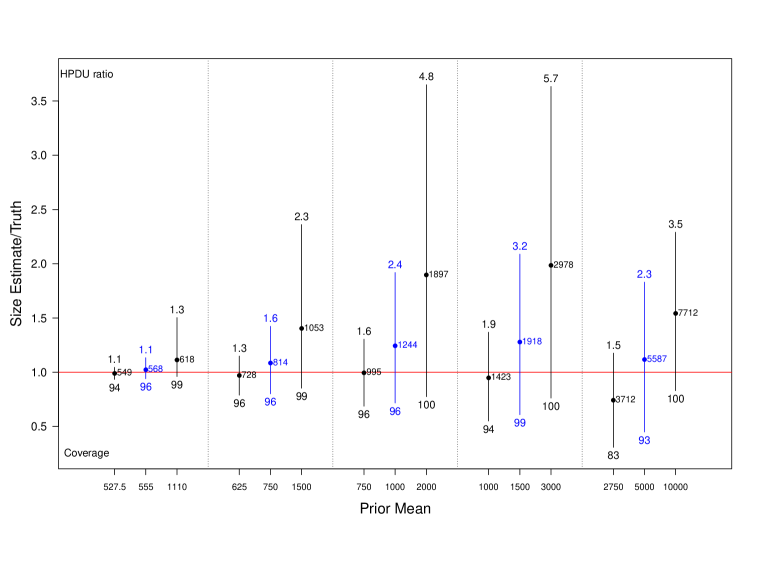
Figure 2: Spread of central 95% of simulated population size estimates (posterior means) for 5 population sizes for low, accurate, and high priors. Dots represent means. Estimates are represented as multiples of the true population size (red line at 1 indicates true population size). Numbers below the bars are coverage rates of 95% HPD intervals, numbers above the bars indicate the widths of these intervals (ratio of median upper bound to truth).

When the prior is correct (blue lines), average point estimates are reasonably close in all cases. There is a small amount of positive bias. This is because of the successive sampling (SS) approximation to the true link-tracing network sampling process. In SS, the next unit sampled would be chosen with probability proportional to unit size from among all unsampled units. In RDS, the network structure constrains the selection of each subsequent unit, with the effect that the decrease in sampled unit sizes over time is less sharp than in successive sampling, leading to a slight positive bias in the population size estimates. The coverage rates of nominal 95% credible intervals are about right in the case of accurate prior information.

Because there is limited information regarding population size in the RDS samples, results are affected by the choice of prior mean, with greater impact for smaller sample fractions. This is because smaller sample fractions entail less exhaustion of the target population and therefore less information in the data about population size.

The coverage rates for the 95% HPD regions for cases of prior mis-specification range from 83% to 100%, with higher coverage rates for higher prior means. These intervals can be quite wide. Because of the lower bound induced by the sample size, interval width is largely determined by the upper limits. The numbers above the bars in Figure 2 represent the median across each set of 200 simulations of the upper limit of the HPD intervals, represented as a multiple of the true population size. When the population size is close to the sample size, intervals are quite tight, while smaller sample fractions yield intervals that are often very large, with median upper point 3.2 times the true population size for $N=1500$, and even wider (5.7 times) with higher prior mean of $3000$.

3.2 Impact of Network Structure

Figure 3 summarizes the results of varying the levels of homophily and differential activity, for varying prior specifications, all for populations of size 1000. Each pair of columns provides comparison across two levels of homophily ($\alpha$). The paired columns are very similar, in both point and interval estimates, and across all levels of differential activity. This suggests that under a broad range of circumstances, homophily does not have a strong first-order impact.

There does appear, however, to be a first order impact of differential activity ($\omega=0.5$ and $\omega=2$), across levels of homophily. By systematically varying mean degree across infection groups, differential activity increases the variation in the unit size distribution, increasing the rate of decline in sampled unit sizes, and therefore providing more information about population size, resulting in better point estimates. Note how the prior mean 2000 cases have point estimates far closer to the truth when $\omega=2$ as compared to $\omega=1$. The credible intervals (HPDU ratios) are also typically smaller for $\omega\not=1$ cases, without substantial reduction in the coverage rates.

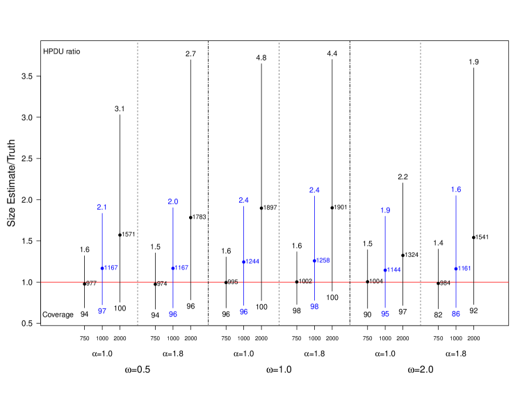
Figure 3: Spread of central 95% of simulated population size estimates (posterior means) for population size 1000 for low, accurate, and high priors, with varying levels of homophily ($\alpha$) and differential activity ($\omega$). The legend is the same as Figure 2.

3.3 Estimation of Population Proportions

RDS is typically conducted in the interest of estimating population features such as population proportions. Earlier estimators based on RDS data assumed the population size was very large with respect to the sample size, so that finite population effects could be ignored. The more recent estimator which introduces the successive sampling (SS) approximation on which this paper is based (Gile, 2011), however, includes a finite population adjustment, but assumes that the population size is known. It is natural, therefore, to use the approach to population size estimation introduced in this paper to provide a population size estimate for use in the prevalence estimator in Gile (2011). Hence this section considers estimates of infection prevalence using the SS estimator. This section compares results using the prior mean as the population size to results using the posterior mean.

Figure 4 shows the SS results for the same simulation conditions as Figure 3. Absent differential activity (Figure 4, middle 2 columns), there is little difference between results using the prior and posterior means. This is because the SS estimator re-weights the sample based on unit sizes (degrees) and the assumed population size. Absent differential activity, the infected and uninfected subsamples will have similar degree distributions, and therefore be similarly affected by any aberrations in the unit weights.

In the presence of differential activity, inaccurate population size estimates introduce bias in the point estimates given by the successive sampling estimator (see Gile, 2011). The first and last two columns of Figure 4 compare prevalence estimates based on the prior and posterior means for cases with strong differential activity. Consistent with Gile (2011), the dashed bars, corresponding to estimates using the prior mean, show substantial bias when the population size is inaccurate. This is due to imperfect adjustment for finite population effects. The primary advantage of estimates based on the posterior mean is the reduction of this dramatic bias. The cost of this reduction, however, is increased variance of the estimator, resulting in higher MSE in cases with small finite population biases, such as when the prior mean is correct. Note that because the bootstrap standard error estimator associated with the successive sampling estimator does not account for uncertainty in the population size, coverage rates can be dramatically low, especially for the estimator based on the prior mean.

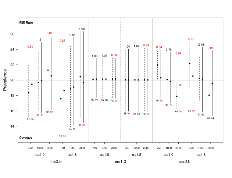
Figure 4: Spread of central 95% of simulated prevalence estimates for population size 1000, with varying levels of homophily ($\alpha$) and differential activity ($\omega$). Solid lines represent prevalence estimates based on the posterior mean, dashed lines represent comparable estimates using the prior mean. Relative efficiency (MSE posterior/MSE prior) is given above each bar, and the coverage of nominal 95% confidence intervals is below each bar. The true prevalence is 0.2 (blue line).

4 Application: Estimating the numbers of those most at risk for HIV in Cities in El Salvador

Overall, El Salvador is a country with low HIV prevalence. As of 2010, the adult HIV prevalence was estimated at 0.8% (UNAIDS/WHO, 2010). However the virus remains a significant threat in groups who practice high-risk behaviors, such as female sex workers (FSW) and men who have sex with men (MSM) (Morales-Miranda et al., 2007; Soto et al., 2007).

This section analyses two studies from data collected in 2010 as part of a series of RDS studies of populations most at risk for HIV across major El Salvadorian cities (Paz-Bailey et al., 2011).

The first case is a study of FSW in the department of Sonsonate, which had a population of about 540,000 in 2008 (Guardado et al., 2010). This study began with 5 seeds and continued until wave 9, with 11 samples from wave 8 and 5 from wave 9, and a total of 184 samples. The average wave number was 3.8. A graph of the recruitment is given in the Supplementary Materials.

As is typical in these settings, the number of female sex workers in Sonsonate is unknown. The public health officials use the UNAIDS national HIV estimation work group recommendation to estimate the number of FSW based on a percent from the total adult female population (UNAIDS/WHO, 2003). In 2009, this group estimated that FSW constitute 0.4%-0.8% of the urban female population 15-49 years of age (139,804) (de Estadistica y Censos, 2007; Paz-Bailey et al., 2011). The range for Sonsonate is then 560 to 1120 FSW.

Estimates of the total number of FSW in Sonsonate are calculated with three different priors. The first prior is constant over the range of population sizes where the likelihood is non-negligible. Figure 5 plots both the prior and posterior distributions. The peakedness of the posterior shape indicates that there is information in the data about the population size, with a mode of around 1250 FSW. The UNAIDS guidelines (purple lines) fall in the mid to low part of the posterior distribution, are broadly consistent with it, and fall within the 95% HPD interval (blue lines).

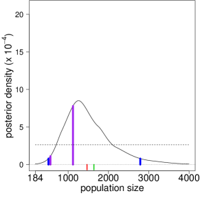
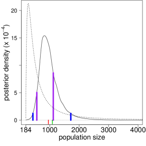
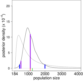
Figure 5: Posterior distribution for the number of female sex workers in Sonsonate based on three prior distributions for the population size: flat, matching the midpoint UNAIDS estimate, and interval-matching the UNAIDS estimate. The prior is dashed. The red mark is at the posterior median. The green mark is at the posterior mean. The blue lines are at the lower and upper bounds of the 95% highest-probability-density interval. The purple lines demark the lower and upper UNAIDS guidelines.

The second prior places the prior mean at the mid-point of the UNAIDS suggested range $0.6\%\times{139804}=838$. Figure 5 plots this prior and the resulting posterior. The mean, median and mode of the posterior fall within the UNAIDS guidelines (purple lines) and these guidelines fall within the the 95% HPD interval. As expected, this prior results in more mass in the posterior in the area of the UNAIDS estimates.

As UNAIDS provides a range of values, it may be useful to specify a prior based on multiple points in that range. The class of priors described by (15) allows the flexibility to choose a prior that reflects a range of values. In this case, two parameters $(\alpha,\beta)$ are chosen so that the prior mean is the midpoint of the range ($0.6\%$) and the lower quartile of the prior is the lower UNAIDS estimate ($0.4\%$). Figure 5 plots this prior and resulting posterior distribution. This distribution has a mode at about 1000 FSW, and a 95% HPD interval from 481 to 1998 FSW.

The above analysis is now repeated for a study of MSM in San Miguel. In 2009, the UNAIDS national HIV estimation work group estimated the number of MSM in El Salvador at 2%-5% of the urban male population 15-49 years of age (148,489) (UNAIDS/WHO, 2003; de Estadistica y Censos, 2007; Paz-Bailey et al., 2011). The range for San Miguel is then 2970 to 7425 MSM.

Figure 6 shows the same three prior specifications as the previous case. Figure 6 plots the posterior distribution and the prior when the prior is constant over the range of population sizes where the likelihood is non-negligible. The peakedness of the posterior shape again indicates that there is information in the data about the size, but it is diffuse and has a long upper tail compared to that for the FSW. The UNAIDS guidelines (purple lines) fall in the mid to upper part of the distribution, and are well within the 95% HPD interval (blue lines).

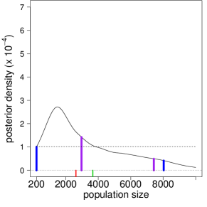
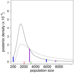
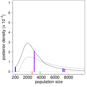
Figure 6: Posterior distribution for the number of MSM in San Miguel based on three prior distributions for the population size: flat, matching the midpoint UNAIDS estimate, and interval-matching the UNAIDS estimate. The legend is the same as Figure 5.

Figure 6 plots the posterior distribution based on the prior with mean the mid-point of the UNAIDS suggested value $3.5\%\times{148489}=5197$. The majority of the posterior is below the UNAIDS estimates as the prior pulls in the larger values while the 95% interval mostly covers them.

Figure 6 plots the posterior distribution based on the prior fixing the mean at the midpoint of the range ($3.5\%$) and the lower point ($2\%$) at the lower quartile. This prior contains the most information from the UNAIDS work group and hence is perhaps the best choice. The resulting posterior distribution has a mode at about 2100 MSM, and a 95% HPD interval from 200 to 7048 MSM. Thus this method yields an estimate of the number of MSM in San Miguel with a wide interval.

Another reference point for population size estimates in El Salvadorian cities can be extrapolated from the results of another study in San Salvador. In this study, capture-recapture was used to estimate the number of MSM and FSW in San Salvador in 2008 (Paz-Bailey et al., 2011). This approach required the distribution of tokens (e.g., key chains) throughout the population followed by a recapture step with a follow-up survey. Paz-Bailey et al. (2011) estimate that the size of the FSW population in San Salvador is almost double the UNAIDS figures (1.4%). This population proportion in Sonsonate would translate to 2079 FSW, close to the posterior mean of the proposed method for the flat prior, but in the upper tail of the posteriors based on priors based on the UNAIDS guidelines. Paz-Bailey et al. (2011) estimate that the size of the MSM population in San Salvador is close to the UNAIDS figures (3.4%). This is somewhat high but comparable to the MSM results in Figure 6. Thus the results here are largely comparable to those of Paz-Bailey et al. (2011) when they differ from the UNAIDS guidelines.

5 Discussion

The primary contribution of this paper is a method to estimate population size from RDS data alone. All existing methods require at least two data sources, and strong assumptions about their dependence structure. Intuitively, when unit sizes are associated with sampling probability, a systematic decline in observed unit sizes over time is indicative of the depletion of the available population. As described in this paper, a successive sampling approximation to the RDS process leverages this change in observed sizes to estimate the size of the hidden population. These data were previously unexploited in the estimation of the size of hard-to-reach human populations. Because RDS is designed for inference in hard-to-reach populations, such data often exist in precisely the populations where population size is unknown but of great interest. Thus this method provides additional important information, that is, an estimate of population size, at no extra cost. Furthermore, the Bayesian framework of this work allows for easy incorporation of informative prior information or data from other sources.

The main limitation of the proposed method is the small amount of information on population size available in many RDS samples, with less information available in smaller sample fractions. In cases with little information, this method results in very large interval estimates in order to obtain reasonable frequentist coverage properties. However, existing methods are also subject to great uncertainty, even though they typically require additional data collection. Often these methods lead to apparently conflicting results because they poorly estimate measures of uncertainty (Salganik et al., 2011). The advantage of the proposed method is that it uses existing data and accurately assesses the degree of uncertainty in $N$ over a wide range of practical situations. Results from the two cases in El Salvador provide estimates compatible with UNAIDS guideline estimates as well as capture/recapture estimates of population sizes.

This method is also useful for estimators of population characteristics that require an estimate of the population size. The simulation study demonstrates that using population size estimates from the proposed method in the SS estimator (Gile, 2011) works well and is particularly helpful in conditions of strong differential activity and larger sample fractions.

The framework developed in this paper is designed to be a foundation upon which other approaches to population size estimation can build. In particular it is designed to facilitate combination with data from multiple methods (e.g., direct surveys, capture-recapture, network scale-up and multiplier). The posterior from the approach in this paper can be used as a prior for combination with information from these alternative methods. Thus this methodology will lead to coherent inference that can be incrementally improved in a constructive way.

While the methods in this paper have been applied to data collected via RDS, we note that the approach is general and applies to data collected via successive sampling. Hence the method has broad applicability (Andreatta and Kaufman, 1986; Nair and Wang, 1989; Bickel et al., 1992).

The R package implementing the methods developed in this paper (Handcock, 2011) will be available on CRAN (R Development Core Team, 2011).

6 Supplementary Materials

Inferential and Computation:

This supplement presents specifics of the estimation algorithms, variations of models for the unit size distribution, a proof of the non-amenability of RDS, and the recruitment graph for the study of female sex workers in El Salvador.

References

- Abdul-Quader et al. (2006) Abdul-Quader, A. S., D. D. Heckathorn, C. McKnight, H. Bramson, C. Nemeth, K. Sabin, K. Gallagher, and D. C. D. Jarlais (2006). Effectiveness of respondent-driven sampling for recruiting drug users in New York City: Findings from a pilot study. Journal of Urban Health 83, 459–476.
- Andreatta and Kaufman (1986) Andreatta, G. and G. M. Kaufman (1986). Estimation of finite population properties when sampling is without replacement and proportional to magnitude. Journal of the American Statistical Association 81(395), 657–666.
- Bao et al. (2010) Bao, L., A. E. Raftery, and A. Reddy (2010). Estimating the size of populations at high risk of HIV in Bangladesh using a Bayesian hierarchical model. Department of statistics technical report no 573, University of Washington.
- Barndorff-Nielsen (1978) Barndorff-Nielsen, O. E. (1978). Information and Exponential Families in Statistical Theory. New York: Wiley.
- Berchenko and Frost (2011) Berchenko, Y. and S. D. W. Frost (2011). Capture-recapture methods and respondent-driven sampling: their potential and limitations. Sexually Transmitted Infections 87(4), 267–268.
- Bernard et al. (2010) Bernard, H. R., T. Hallett, A. Iovita, E. C. Johnsen, R. Lyerla, C. McCarty, M. Mahy, M. J. Salganik, T. Saliuk, O. Scutelniciuc, G. A. Shelley, P. Sirinirund, S. Weir, and D. F. Stroup (2010). Counting hard-to-count populations: the network scale-up method for public health. Sexually Transmitted Infections 86(Suppl 2), ii11–ii15.
- Bernhardt et al. (2006) Bernhardt, A., D. Heckathorn, R. Milkman, and N. Theodore (2006). Documenting unregulated work: A survey of workplace violations in New York City. The Future of Work.
- Bickel et al. (1992) Bickel, P. J., V. N. Nair, and P. C. C. Wang (1992). Nonparametric inference under biased sampling from a finite population. The Annals of Statistics 20(2), 853–878.
- de Estadistica y Censos (2007) de Estadistica y Censos, D. G. (2007). Vi censo de poblacion y v de vivienda El Salvador. Technical report, Ministerio de Economia de El Salvador.
- Felix-Medina and Thompson (2004) Felix-Medina, M. H. and S. K. Thompson (2004). Combining link-tracing sampling and cluster sampling to estimate the size of hidden populations. Journal of Official Statistics 20, 19–38.
- Fienberg et al. (1999) Fienberg, S. E., M. S. Johnson, and B. W. Junker (1999). Classical multilevel and bayesian approaches to population size estimation using multiple lists. Journal of the Royal Statistical Society: Series A (Statistics in Society) 162(3), 383–405.
- Frank and Snijders (1994) Frank, O. and T. A. B. Snijders (1994). Estimating the size of hidden populations using snowball sampling. Journal of Official Statistics 10(1), 53–67.
- Gile (2011) Gile, K. J. (2011). Improved inference for respondent-driven sampling data with application to HIV prevalence estimation. Journal of the American Statistical Association 106, 135–146.
- Gile and Handcock (2010) Gile, K. J. and M. S. Handcock (2010). Respondent-driven sampling: An assessment of current methodology. Sociological Methodology 40, 285–327.
- Gile and Handcock (2011) Gile, K. J. and M. S. Handcock (2011). Network model-assisted inference from respondent-driven sampling data. ArXiv Preprint.
- Guardado et al. (2010) Guardado, M. E., J. Creswell, E. Monterroso, et al. (2010). Encuesta centroamericana de vigilancia de comportamiento sexual y prevalencia de VIH/ITS en poblaciones vulnerables, hombres que tienen sexo con hombres, trabajadoras sexuales y personas con VIH, ECVC El Salvador. Research report, Minisiterio de Salud de El Salvador.
- Handcock (2011) Handcock, M. S. (2011). size: Estimating Population Size from Discovery Models using Successive Sampling Data. Los Angeles, CA: Hard-to-Reach Population Methods Research Group. R package version 0.20.
- Handcock and Gile (2010) Handcock, M. S. and K. J. Gile (2010). Modeling networks from sampled data. Annals of Applied Statistics 272(2), 383–426.
- Handcock et al. (2003) Handcock, M. S., D. R. Hunter, C. T. Butts, S. M. Goodreau, and M. Morris (2003). statnet: Software Tools for the Statistical Modeling of Network Data. Seattle, WA: Statnet Project http://statnet.org/. R package version 2.0.
- Heckathorn (1997) Heckathorn, D. D. (1997). Respondent-driven sampling: A new approach to the study of hidden populations. Social Problems 44, 174–199.
- Heckathorn (2002) Heckathorn, D. D. (2002). Respondent-driven sampling II: Deriving valid population estimates from chain-referral samples of hidden populations. Social Problems 49(1), 11–34.
- Heckathorn and Jeffri (2001) Heckathorn, D. D. and J. Jeffri (2001). Finding the beat: Using respondent-driven sampling to study jazz musicians. Poetics 28, 307–329.
- Johnston et al. (2008) Johnston, L. G., M. Malekinejad, C. Kendall, I. M. Iuppa, and G. W. Rutherford (2008). Implementation challenges to using respondent-driven sampling methodology for HIV biological and behavioral surveillance: Field experiences in international settings. AIDS and Behavior 12, 131–141.
- Johnston et al. (2011) Johnston, L. G., D. Prybylski, H. F. Raymond, A. Mirzazadeh, C. Manopaiboon, and W. McFarland1 (2011). Incorporating the service multiplier method in respondent driven sampling surveys to estimate the size of hidden and hard-to-reach populations: Case studies from around the world. Unpublished manuscript, University of California, San Francisco.
- Morales-Miranda et al. (2007) Morales-Miranda, S., G. Paz-Bailey, B. Alvarez, et al. (2007). Behavioral and HIV survey among female sex workers and men who have sex with men in Honduras using respondent driven sampling. Technical report, University of Valle of Guatemala.
- Nair and Wang (1989) Nair, V. N. and P. C. C. Wang (1989). Maximum likelihood estimation under a successive sampling discovery model. Technometrics 31(4), 423–436.
- Niccolai et al. (2010) Niccolai, L. M., S. V. Verevochkin, O. V. Toussova, E. White, R. Barbour, A. P. Kozlov, and R. Heimer (2010). Estimates of HIV incidence among drug users in St. Petersburg, Russia: continued growth of a rapidly expanding epidemic. The European Journal of Public Health.
- Paz-Bailey et al. (2011) Paz-Bailey, G., J. O. Jacobson, M. E. Guardado, F. M. Hernandez, A. I. Nieto, M. Estrada, and J. Creswell (2011). How many men who have sex with men and female sex workers live in El Salvador? using respondent-driven sampling and capture-recapture to estimate population sizes. Sexually Transmitted Infections 87(4), 279–282.
- R Development Core Team (2011) R Development Core Team (2011). R: A Language and Environment for Statistical Computing. Vienna, Austria: R Foundation for Statistical Computing. ISBN 3-900051-07-0, Version 2.14.
- Rocchetti et al. (2011) Rocchetti, I., J. Bunge, and D. Böhning (2011). Population size estimation based upon ratios of recapture probabilities. Annals of Applied Statistics 5(2B), 1512–1533.
- Salganik et al. (2011) Salganik, M. J., D. Fazito, N. Bertoni, A. H. Abdo, M. B. Mello, and F. I. Bastos (2011). Assessing network scale-up estimates for groups most at risk of HIV/AIDS: Evidence from a multiple-method study of heavy drug users in Curitiba, Brazil. American Journal of Epidemiology 174(10), 1190–1196.
- Salganik and Heckathorn (2004) Salganik, M. J. and D. D. Heckathorn (2004). Sampling and estimation in hidden populations using respondent-driven sampling. Sociological Methodology 34, 193–239.
- Shmueli et al. (2005) Shmueli, G., T. P. Minka, J. B. Kadane, S. Borle, and P. Boatwright (2005). A useful distribution for fitting discrete data: revival of the Conway-Maxwell-Poisson distribution. Journal of the Royal Statistical Society: Series C (Applied Statistics) 54(1), 127–142.
- Snijders et al. (2006) Snijders, T. A. B., P. Pattison, G. L. Robins, and M. S. Handcock (2006). New specifications for exponential random graph models. Sociological Methodology 36, 99–153.
- Soto et al. (2007) Soto, R. J., A. E. Ghee, C. A. Nunez, R. Mayorga, K. A. Tapia, S. G. Astete, J. P. Hughes, A. L. Buffardi, S. E. Holte, K. K. Holmes, and the Estudio Multicentrico Study Team (2007). Sentinel surveillance of sexually transmitted infections/HIV and risk behaviors in vulnerable populations in 5 Central American countries. Journal of Acquired Immune Deficiency Syndromes and Human Retrovirology 46, 101–111.
- Tomas and Gile (2010) Tomas, A. and K. J. Gile (2010). The effect of differential recruitment, non-response and non-recruitment on estimators for respondent-driven sampling. ArXiv Preprint.
- UNAIDS (2009) UNAIDS (2009). Estimating National Adult Prevalence of HIV-1 in Concentrated Epidemics. Technical report, UNAIDS - Joint United Nations Programme on HIV/AIDS.
- UNAIDS and World Health Organization (2010) UNAIDS and World Health Organization (2010). Guidelines on estimating the size of populations most at risk to HIV. Technical Report UNAIDS/00.03E, UNAIDS - Joint United Nations Programme on HIV/AIDS.
- UNAIDS/WHO (2003) UNAIDS/WHO (2003). Estimating the size of populations at risk for HIV: Issues and methods. Technical report, UNAIDS/WHO Working Group on HIV/AIDS.
- UNAIDS/WHO (2010) UNAIDS/WHO (2010). HIV/AIDS health profile of El Salvador. Technical report, UNAIDS/WHO Working Group on HIV/AIDS.
- van Duijn et al. (2009) van Duijn, M. A. J., M. S. Handcock, and K. J. Gile (2009). A framework for the comparison of maximum pseudo likelihood and maximum likelihood estimation of exponential family random graph models. Social Networks 31, 52–62.
- Volz and Heckathorn (2008) Volz, E. and D. D. Heckathorn (2008). Probability based estimation theory for respondent driven sampling. Journal of Official Statistics 24(1), 79–97.
- West (1996) West, M. (1996). Inference in successive sampling discovery models. Journal of Econometrics 75, 217–238.