Study of the anomalous cross-section lineshape of $e^{+}e^{-}\to D\bar{D}$ at $\psi(3770)$ with an effective field theory

Abstract

We study the anomalous cross-section lineshape of $e^{+}e^{-}\rightarrow D\bar{D}$ with an effective field theory. Near the threshold, most of the $D\bar{D}$ pairs are from the decay of $\psi(3770)$. Taking into account the fact that the nonresonance background is dominated by the $\psi(2S)$ transition, the produced $D\bar{D}$ pair can undergo final-state interactions before the pair is detected. We propose an effective field theory for the low-energy $D\bar{D}$ interactions to describe these final-state interactions and find that the anomalous lineshape of the $D\bar{D}$ cross section observed by the BESII collaboration can be well described.

As the first charmonium state above the $D\bar{D}$ threshold, the resonance $\psi(3770)$ is different from other charmonia with lower masses. Because the $\psi(3770)$ decay into the open charm $D\bar{D}$ is allowed by the Okubo-Zweig-Iizuka (OZI) rule, this dominant decay mode leads to a broad width up to $27.2\pm 1.0$ MeV [1]. Obviously, the direct production process of $e^{+}e^{-}\to\psi(3770)\rightarrow D\bar{D}$ is useful for the study of the properties of $\psi(3770)$. In Ref. [2], BESII collaboration reported an anomalous behavior of the cross-section lineshape at the $\psi(3770)$ mass region in $e^{+}e^{-}\rightarrow D\bar{D}$ that cannot be described by a simple Breit-Winger of $\psi(3770)$. Such an observation has inspired interesting theoretical discussions [3, 4, 5, 6]. In particular, it was found that the interfering effect between $\psi(3770)$ and $\psi(2S)$ plays a very important role in understanding the anomalous lineshape of $D\bar{D}$ at the $\psi(3770)$ resonance [3, 4]. Such an interference can be recognized by a relative phase factor $e^{i\phi}$, which is introduced between these two resonances, and the phase angle $\phi$ must be large to describe the anomalous $D\bar{D}$ lineshape.

In principle, the phase factor $e^{i\phi}$ can come from the final-state interactions of $D\bar{D}$. Thus, it should be interesting to study the $D\bar{D}$ anomalous lineshape using an effective field theory to describe the $D\bar{D}$ final-state interactions. This forms our motivation for this work. Near the threshold, the $D\bar{D}$ pair produced in $e^{+}e^{-}\rightarrow D\bar{D}$ comes from the decay of the $\psi(3770)$ and other nonresonance background processes. Once the $D\bar{D}$ pair is produced, it could undergo final-state interactions before it converts into the final observed $D\bar{D}$ state. This phenomenon could explain the relative phase between the $\psi(3770)$ and other non-$\psi(3770)$ amplitude and provide a description of the $D\bar{D}$ lineshape. We note that there are several cases in which the final-state interactions play important roles in the understanding of the cross-section lineshapes [7, 8, 9, 10].

It is well known that an effective field theory is a useful tool to study the low-energy hadron interactions. An effective field theory utilizes the Tailor expansion of the small ratio between the typical small scale $p$ and the cutoff scale $\Lambda$. For example, in Chiral Perturbation Theory (ChPT), $p$ is the momentum of the low-energy pion or pion mass, whereas $\Lambda=M_{\rho(770)}$ sets the cutoff scale of this effective theory. An effective field theory for the low-energy $D\bar{D}$ is different from that for the low-energy $\pi\pi$ interaction because the $\psi(3770)$ should be included explicitly into the effective Lagrangian. In addition to the three-vector momentum of the $D$ ($\bar{D}$) meson, another small scale, $\delta=M_{\psi(3770)}-2M_{D}\approx 40$ MeV, also appears in the effective theory. This additional small scale will make the power counting different from that in ChPT. A systematic development of the effective field theory with resonances as intermediate states is still under exploration, and interesting discussions on this subject can be found in Refs. [11, 12].

In this work, we use the effective field theory to study the $D\bar{D}$ interaction to understand the dynamic details of the anomalous cross-section lineshape observed by the BESII Collaboration [2].

At the beginning, we assume that the production of $D\bar{D}$ in $e^{+}e^{-}$ annihilation can be approximated by the vector meson dominance (VMD). This assumption means that the cross section for $e^{+}e^{-}\rightarrow D\bar{D}$ is dominated by intermediate vector meson productions via $e^{+}e^{-}\rightarrow\gamma^{\ast}\rightarrow\mathcal{R}_{i}\rightarrow D\bar{D}$, where $\mathcal{R}_{i}$ denotes any vector meson with an isospin of $I=0$ or $I=1$. However, it is impossible to sum the contributions from all of the $\mathcal{R}_{i}$ in reality. As a reasonable approximation, one can include the contributions from the vector mesons in the vicinity of the considered energy region but neglect those far off-shell vector mesons. In the energy region of the BES data from 3.74 GeV to 3.8 GeV, one can expect that $\psi(3770)$ plays the most important role among all of the $\mathcal{R}_{i}$, whereas the contributions from all the other $\mathcal{R}_{i}$ can be treated as background. As shown in Ref. [3], the contribution from $\psi(2S)$ dominates the background, whereas the contributions from other states are negligible. Therefore, we only include the contributions from the resonances $\psi(3770)$ and $\psi(2S)$ and neglect those from the other resonances. Namely, $\psi(2S)$ would be the main background near the $D\bar{D}$ threshold.

In VMD [13, 14], the coupling between the vector meson and a virtual photon can be described as

$$\mathcal{L}_{V\gamma}=\frac{eM_{V}^{2}}{f_{V}}V_{\mu}A^{\mu},$$ (1)

where $V_{\mu}$ is the vector meson field, $A_{\mu}$ is the photon field, and $M_{V}$ is the mass of the vector meson. Setting the electron mass to $m_{e}\approx 0$, the coupling can be obtained as

$$\frac{e}{f_{V}}=\left[\frac{3\Gamma_{ee}}{\alpha M_{V}}\right]^{1/2},$$ (2)

where $\Gamma_{ee}$ is the electron-position decay width of $V_{\mu}$ and $\alpha=1/137$ is the fine-structure constant.

Once the $D\bar{D}$ pair is produced from the decay of the vector meson $\psi(3770)$ or $\psi(2S)$, the pair can undergo final-state interactions through the rescattering processes $D\bar{D}\rightarrow D\bar{D}\rightarrow\cdots\rightarrow D\bar{D}$, which can be described by the effective field theory. In the energy region of interest, the three-vector momentum $p$ of the $D(\bar{D})$ meson is small. Thus, it is possible to construct an effective field theory for the low-energy $D\bar{D}$ interactions by making use of the expansion of the small momentum $p$. Because the mass of $\psi(3770)$ is just above the threshold of $D\bar{D}$, we need to include $\psi(3770)$ explicitly in the formulation. Near the threshold, the $D$($\bar{D}$) meson can be treated as nonrelativistic. Thus, the interaction Lagrangian for the $D\bar{D}$ system with the quantum number $J^{PC}=1^{--}$ can be constructed as

$$\delta\mathcal{L} = \mathcal{L}_{\psi D\bar{D}}+\mathcal{L}_{(D\bar{D})^{2}}$$

$$\mathcal{L}_{\psi D\bar{D}} = ig_{\psi D\bar{D}}\{D^{\dagger}\bm{\nabla}\bar{D}-\bm{\nabla}D^{\dagger}\bar{D}\}\cdot\bm{\psi}+ig_{\psi D\bar{D}}\{\bar{D}^{\dagger}\bm{\nabla}D-\bm{\nabla}\bar{D}^{\dagger}D\}\cdot\bm{\psi},$$

$$\mathcal{L}_{(D\bar{D})^{2}} = f_{1}\{D^{\dagger}\bm{\nabla}\bar{D}-\bm{\nabla}D^{\dagger}\bar{D}\}\cdot\{\bm{\nabla}\bar{D}^{\dagger}D-\bar{D}^{\dagger}\bm{\nabla}D\}$$

$$+f_{3}\{D^{\dagger}\tau^{i}\bm{\nabla}\bar{D}-\bm{\nabla}D^{\dagger}\tau^{i}\bar{D}\}\cdot\{\bm{\nabla}\bar{D}^{\dagger}\tau^{i}D-\bar{D}^{\dagger}\tau^{i}\bm{\nabla}D\}+\cdots,$$

$$\mbox{with}\ \ \ D = \left(\begin{array}[]{c}D^{0}\\ D^{+}\\ \end{array}\right),\ \ \ \bar{D}=\left(\begin{array}[]{c}\bar{D}^{0}\\ D^{-}\\ \end{array}\right),$$ (7)

where $\psi$ is the field operator of $\psi(3770)$; $D$ ($\bar{D}^{\dagger}$) annihilates a $D$($\bar{D}$) meson; $D^{\dagger}$ ($\bar{D}$) creates a $D$($\bar{D}$) meson; $\tau^{i}$ is the Pauli matrix, and the ellipsis denotes other contact terms with more derivatives that are higher order terms. The first term in $\mathcal{L}_{(D\bar{D})^{2}}$ accounts for the interaction in the isospin singlet channel, and the second term accounts for the isospin triplet channel. The contributions from other resonances, which are not included in the Lagrangian, can be saturated into the contact terms $\mathcal{L}_{(D\bar{D})^{2}}$. Therefore, we take the coefficients such as $f_{1},f_{3}$ to be complex, where the imaginary parts of these terms come from the width of the saturated resonances and the $D\bar{D}$ annihilation effect. With isospin symmetry, we only have to consider the terms for the isospin singlet channel in $\mathcal{L}_{(D\bar{D})^{2}}$ to study the $D\bar{D}$ final-state interactions because the $D\bar{D}$ pair comes from the decay of $\psi(3770)$ and $\psi(2S)$ in our approach.

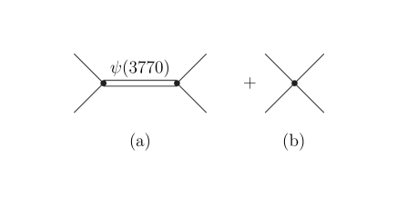
Figure 1: Tree diagrams for $D\bar{D}\rightarrow D\bar{D}$. (a) $D\bar{D}\rightarrow\psi(3770)\rightarrow D\bar{D}$, (b) contact interaction.

Now we come to the discussion of the power counting of this effective field theory. The tree-level diagrams for the $D\bar{D}$ elastic scattering are shown in Fig. 1. Near the $D\bar{D}$ threshold, the denominator of the $\psi(3770)$ propagator can be expressed as

$$P(\psi) = \frac{1}{s-M_{\psi}^{2}+iM_{\psi}\Gamma_{\psi}^{\mbox{non-}D\bar{D}}}$$ (8)

$$\approx \frac{1}{(2M_{D}+p^{2}/M_{D})^{2}-M_{\psi}^{2}+iM_{\psi}\Gamma_{\psi}^{\mbox{non-}D\bar{D}}}$$

$$= \frac{1}{4p^{2}+4M_{D}^{2}-M_{\psi}^{2}+iM_{\psi}\Gamma_{\psi}^{\mbox{non-}D\bar{D}}+\mathcal{O}(p^{4})},$$

where $p$ is the magnitude of the three-vector momentum of the $D$($\bar{D}$) meson in the overall center-of-mass frame, $\Gamma_{\psi}^{\mbox{non-}D\bar{D}}$ denotes the non-$D\bar{D}$ decay width of $\psi(3770)$, and $M_{\psi}$ is the mass of $\psi(3770)$. The $D\bar{D}$ decay width of $\psi(3770)$ will be included through the summation of the D meson loops in the following. Because $\psi(3770)$ is close to the threshold of $D\bar{D}$, we expect that $P(\psi)$ is at $\mathcal{O}(p^{-2})$. Taking the momentum power of the $\psi D\bar{D}$ vertex into account, we find that Fig. 1(a) is at $\mathcal{O}(p^{0})$. From the naive power counting, the leading contact terms have two derivatives; hence, these terms are at $\mathcal{O}(p^{2})$. However, in this naive power counting, we have assumed that the coefficients of the contact terms, i.e., $f_{1},\ f_{3},\cdots$, are at order of $\mathcal{O}(p^{0})$. In some cases, especially when there are bound states or resonances near the threshold, the coefficients of the contact terms can be enhanced. For example, in a $NN$ interaction, the S-wave contact terms $C_{S}$ scale as $\mathcal{O}(p^{-1})$[15]. Another example is the $NN$ interaction in ${}^{3}P_{0}$, where the leading contact term $C_{{}^{3}P_{0}}$ can be promoted to $\mathcal{O}(p^{-2})$[16]. It is interesting to study whether the same enhancement mechanism takes place in the $D\bar{D}$ interactions because the resonance $\psi(3770)$ is located near the $D\bar{D}$ threshold. If $f_{1}$ is promoted to $\mathcal{O}(p^{-2})$ as $C_{{}^{3}P_{0}}$ in a $NN$ interaction, then the corresponding tree diagram shown in Fig. 1(b) is at $\mathcal{O}(p^{0})$, which is the same as Fig. 1(a). However, because we do not know the power of $f_{1}$ at the beginning, we then assume that the leading contributions to $D\bar{D}$ elastic scattering come from both Fig. 1(a) and (b). We will use the experiment data to determine $f_{1}$ and see whether this contact term is enhanced. Accordingly, the $D\bar{D}$ scattering amplitude in the specific channel ($J^{PC}=1^{--},I=0$) can be obtained by summing the bubble diagrams as shown in Fig. 2, which is equivalent to solving the Lippmann-Schwinger equation $T=V+\int VGT$ with the $D\bar{D}$ potential truncated at the leading order.

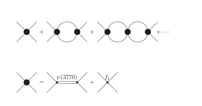
Figure 2: The bubble diagrams for the $D\bar{D}$ interactions where the potential is truncated at the leading order.

Figure 3 illustrates the final-state interactions between the produced $D\bar{D}$. Because we first assume $f_{1}$ is enhanced, which indicates the interaction between $D\bar{D}$ is strong or the $D\bar{D}$ scattering length is large, we will use the power divergent substraction (PDS) scheme proposed by Ref. [15] to describe the large-scattering-length system in our calculations. The loop integrals that we will encounter in Fig. 3 can generally be reduced to

$$\mathcal{I} \equiv (\mu/2)^{4-D}\int\frac{d^{D}\ell}{(2\pi)^{D}}\frac{\vec{\ell}^{2}}{[\ell^{0}-\vec{\ell}^{2}/2M_{D}+i\epsilon]\cdot[E-\ell^{0}-\vec{\ell}^{2}/2M_{D}+i\epsilon]}$$ (9)

$$= -i(\mu/2)^{4-D}\int\frac{d^{(D-1)}\ell}{(2\pi)^{(D-1)}}\frac{\vec{\ell}^{2}}{E-\vec{\ell}^{2}/M_{D}+i\epsilon}$$

$$= iM_{D}(M_{D}E)(-M_{D}E-i\epsilon)^{(D-3)/2}\Gamma(\frac{3-D}{2})\frac{(\mu/2)^{4-D}}{(4\pi)^{(D-1)/2}},$$

where $E=p^{2}/M_{D}$ is the total kinematic energy of the $D\bar{D}$ system. It is clear that this result is convergent in $D=4$ but divergent in $D=3$. With the PDS scheme, we have to remove the $D=3$ pole in the above result by adding the counterterm

$$\delta\mathcal{I}=i\frac{M_{D}(M_{D}E)\mu}{4\pi(D-3)}.$$ (10)

Hence the subtracted integral in $D=4$ reads

$$\mathcal{I}^{PDS}=\mathcal{I}+\delta\mathcal{I}=i\frac{M_{D}}{4\pi}p^{2}(ip+\mu).$$ (11)

Notice that $\mathcal{I}^{PDS}=\mathcal{I}$ at $\mu=0$, which is simply the result in the minimal subtraction (MS) scheme. We can choose $\mu$ to be the typical momentum scale of the $D(\bar{D})$ meson, which is $p\leq 300$ MeV in our calculations.

We can then write down the amplitude for $e^{+}e^{-}\rightarrow D\bar{D}$ as

$$i\mathcal{M}=i\mathcal{M}_{a}+i\mathcal{M}_{b}.$$ (12)

To be more specific, the amplitude for process Fig. 3(a) reads

$$i\mathcal{M}_{a} = -ie^{2}\bar{v}(k_{2})\bm{\gamma}u(k_{1})\cdot({\bm{p}}_{1}-{\bm{p}}_{2})\frac{1}{s}\frac{M_{\psi}^{2}}{f_{\psi}}\frac{1}{s-M_{\psi}^{2}+iM_{\psi}G_{\psi}}g_{\psi D\bar{D}},$$ (13)

with

$$G_{\psi} = \Gamma_{\psi}^{\mbox{non-}D\bar{D}}+\frac{1}{12\pi M_{\psi}}\left(g^{2}_{\psi D\bar{D}}-f_{1}(s-M_{\psi}^{2}+iM_{\psi}\Gamma_{\psi}^{\mbox{non-}D\bar{D}})\right)\left(\frac{|\vec{p}_{D^{0}}|^{3}-i|\vec{p}_{D^{0}}|^{2}\mu}{M_{D^{0}}}+\frac{|\vec{p}_{D^{+}}|^{3}-i|\vec{p}_{D^{+}}|^{2}\mu}{M_{D^{+}}}\right),$$

where $\gamma$ is the Dirac gamma matrix; $k_{1}$ and $k_{2}$ are the incoming momenta of the electron and positron, respectively, and $p_{1}$ and $p_{2}$ are the outgoing momenta of $D$ and $\bar{D}$, respectively. $G_{\psi}$ cannot be simply interpreted as the width of $\psi(3770)$ because this term is a complex number. If we set $f_{1}=0$ and $\mu=0$, then $G_{\psi}=\Gamma_{\psi}=\Gamma_{\psi}^{\mbox{non-}D\bar{D}}+({|\vec{p}_{D^{0}}|^{3}}/{M_{D^{0}}}+{|\vec{p}_{D^{+}}|^{3}}/{M_{D^{+}}}){g^{2}_{\psi D\bar{D}}}/{(12\pi M_{\psi})}$.

The amplitude for Fig. 3(b) can be written as

$$i\mathcal{M}_{b} = -ie^{2}\bar{v}(k_{2})\bm{\gamma}u(k_{1})\cdot({\bm{p}}_{1}-{\bm{p}}_{2})\frac{1}{s}\frac{M_{\psi(2S)}^{2}}{f_{\psi(2S)}}\frac{1}{s-M_{\psi(2S)}^{2}+iM_{\psi(2S)}\Gamma_{\psi(2S)}}\tilde{g}_{\psi(2S)},$$ (15)

with

$$\tilde{g}_{\psi(2S)} = g_{\psi(2S)D\bar{D}}\left[1+i\frac{1}{12\pi}\left(-f_{1}+\frac{g_{\psi D\bar{D}}^{2}}{s-M_{\psi}^{2}+iM_{\psi}\Gamma_{\psi}^{\mbox{non-}D\bar{D}}}\right)\left(\frac{|\vec{p}_{D^{0}}|^{3}-i|\vec{p}_{D^{0}}|^{2}\mu}{M_{D^{0}}}+\frac{|\vec{p}_{D^{+}}|^{3}-i|\vec{p}_{D^{+}}|^{2}\mu}{M_{D^{+}}}\right)\right]^{-1},$$

where the PDG [17] value for the $\psi(2S)$ mass $M_{\psi(2S)}$ can be adopted, and $f_{\psi(2S)}$ can be extracted by Eq. (2) using $\Gamma_{\psi(2S)\rightarrow e^{+}e^{-}}=2.35$ keV [17].

To proceed, we denote the cross section for $e^{+}e^{-}\rightarrow D\bar{D}$ as $\sigma^{B}(s)$, which does not include the initial state radiation (ISR) effect. In reality, for a given energy $\sqrt{s}$, the actual c.m. energy for the $e^{+}e^{-}$ annihilation is $\sqrt{s^{\prime}}=\sqrt{s(1-x)}$ due to the ISR effect, where $xE_{\mbox{beam}}$ is the total energy of the emitted photons. To order $\alpha^{2}$ radiative correction in the $e^{+}e^{-}$ annihilation, the observed cross section $\sigma^{\mbox{obs}}$ at BESII can be related to our result $\sigma^{B}$ through [18]

$$\sigma^{\mbox{obs}}(s)=(1+\delta_{VP})\int_{0}^{1-4M_{D}^{2}/s}dxf(x,s)\sigma^{B}(s(1-x)),$$ (17)

where $(1+\delta_{VP})=1.047$, and the function $f(x,s)$ is given by

$$f(x,s) = \beta x^{\beta-1}\delta^{V+S}+\delta^{H},$$

$$\beta = \frac{2\alpha}{\pi}(\ln\frac{s}{m_{e}^{2}}-1),$$

$$\delta^{V+S} = 1+\frac{3}{4}\beta+\frac{\alpha}{\pi}(\frac{\pi^{2}}{3}-\frac{1}{2})+\frac{\beta^{2}}{24}(\frac{1}{3}\ln\frac{s}{m_{e}^{2}}+2\pi^{2}-\frac{37}{4}),$$

$$\delta^{H} = -\beta(1-\frac{x}{2})+\frac{1}{8}\beta^{2}\left[4(2-x)\ln\frac{1}{x}-\frac{1+3(1-x)^{2}}{x}\ln(1-x)-6+x\right].$$ (18)

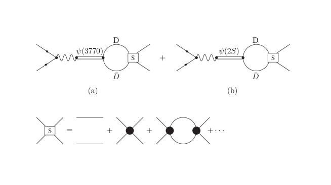
Figure 3: The Feynman diagrams for $e^{+}e^{-}\rightarrow D\bar{D}$ in our approach.

Before fitting the BESII data with Eq. (17), we first discuss our treatment of $\Gamma_{\psi}^{\mbox{non-}D\bar{D}}$. It seems impossible to determine $\Gamma_{\psi}^{\mbox{non-}D\bar{D}}$ definitely in our fitting because $\Gamma_{\psi}^{\mbox{non-}D\bar{D}}$ is always accompanied by $f_{1}$ in our formula, and any change of $\Gamma_{\psi}^{\mbox{non-}D\bar{D}}$ can be compensated by tuning $f_{1}$. The experimental results on the non-$D\bar{D}$ branching ratio of $\psi(3770)$ decay are still controversial [19, 20, 21]. In contrast, the next-to-leading-order (NLO) pQCD calculation expects the non-$D\bar{D}$ decay branching ratio to be at most approximately $5\%$ [22]. Meanwhile, an effective Lagrangian approach estimates that the $D$ meson loop rescatterings into non-$D\bar{D}$ light vector and pseudoscalar mesons leads to approximately 1% non-$D\bar{D}$ branching ratios [23]. A similar calculation by Ref. [24] also confirms such a nonperturbative phenomenon. One also notices that so far, most of the well-measured non-$D\bar{D}$ decay modes of $\psi(3770)$ are found to be rather small. Namely, their branching ratios are either at the order of $10^{-3}-10^{-4}$, or only an upper limit is set [17].

Taking all these facts into account and for the purpose of studying the dominant $D\bar{D}$ channel, we set $\Gamma_{\psi}^{\mbox{non-}D\bar{D}}$ to be zero in our fitting as a leading approximation. We have checked that the fitting results are approximately unchanged even though we set the non-$D\bar{D}$ branching ratio of the $\psi(3770)$ decay to be at the order of several percent.

	MS($\mu=0$)	PDS($\mu=\delta$)	PDS($\mu=m_{\pi}$)	PDS($\mu=300$MeV)
$M_{\psi}(\mbox{GeV})$	$3.7674\pm 0.0044$	$3.7685\pm 0.0056$	$3.7725\pm 0.0046$	$3.7755\pm 0.0041$
$e/f_{\psi}$	$(4.25\pm 0.13)\times 10^{-3}$	$(4.25\pm 0.69)\times 10^{-3}$	$(4.75\pm 0.61)\times 10^{-3}$	$(5.48\pm 0.67)\times 10^{-3}$
$g_{\psi D\bar{D}}$	$15.4\pm 2.7$	$14.6\pm 2.5$	$12.5\pm 2.0$	$10.1\pm 1.4$
$g_{\psi(2S)D\bar{D}}$	$-6.9\pm 3.6$	$-6.3\pm 4.3$	$-6.6\pm 4.1$	$-6.8\pm 3.9$
$f_{1}(\mbox{GeV}^{-2})$	$(2059\pm 534)+i(0\pm 836)$	$(2096\pm 504)+i(76\pm 935)$	$(1871\pm 553)+i(570\pm 726)$	$(1288\pm 452)+i(802\pm 297)$
$\chi^{2}/d.o.f$	$23.4/22\approx 1.06$	$23.3/22\approx 1.06$	$23.3/22\approx 1.06$	$23.4/22\approx 1.06$

Table 1: Fitted parameters and fitting qualities with different $\mu$. Here, we use $\delta=40$ MeV.

The fitted parameters and fitting qualities with $\mu=\delta,\ m_{\pi},\ 300$ MeV are shown in Table i@. For comparison, we also show the result with $\mu=0$, which corresponds to the value in the MS scheme. The result shows that the fitted parameters are insensitive to the choice of $\mu$. Moreover, the real part of $f_{1}$ is large, at the order of $(M_{D}/\delta)^{2}$, which is consistent with our previous assumption. In contrast, the imaginary part of $f_{1}$ is not well determined. Note that the NLO term $f_{1}$ has a comparable magnitude to that of the leading order term. This result suggests that the effective field theory expansion may not be convergent. Thus, the fitting results may not be quantitatively reliable. To have a better understanding of our results, we investigate the dependence of $f_{1}$ on the scattering length $a$ as that was done in Ref. [15]. For the $P$-wave $D\bar{D}$ elastic scattering, we denote the Feynman amplitude as $i\mathcal{A}\cos\theta$, where $\theta$ is the angle between the incoming and outgoing momenta in the c.m. frame. Then, the correlation between $\mathcal{A}$ and the $P$-wave phase shift $\delta$ is

$$\mathcal{A}=\frac{48\pi M_{D}p^{2}}{p^{3}\cot\delta-ip^{3}}.$$ (19)

With the effective range expansion

$$p^{2\ell+1}\cot\delta_{\ell}(p)=\frac{-1}{a_{\ell}}+\frac{r_{\ell}}{2}p^{2}+\mathcal{O}(p^{4}),$$ (20)

and taking the case of $P$-wave scattering ($\ell=1$), we then obtain

$$\mathcal{A}=\frac{48\pi M_{D}p^{2}}{-\frac{1}{a}+\frac{r_{0}}{2}p^{2}-ip^{3}+\mathcal{O}(p^{4})}.$$ (21)

For simplicity and only illustrating some aspects of the effective field theory, we ignore the $\psi(3770)$ and consider a $D\bar{D}$ effective theory with only the contact terms. Accordingly, the tree-level amplitude for the $P$-wave scattering can be written as

$$i\mathcal{A}_{tree}=i\sum_{n=1}^{\infty}C_{2n}p^{2n}.$$ (22)

For the isospin $I=0$ channel, we have the coefficient of the leading contact term $C_{2}=8f_{1}$. The full amplitude can then be obtained by summing over all the bubble diagrams as shown in Fig. 2. The amplitude becomes

$$\mathcal{A}=\frac{\sum C_{2n}p^{2n}}{1-\frac{ip+\mu}{48\pi M_{D}}\sum C_{2n}p^{2n}}.$$ (23)

Using the fact that the amplitude $\mathcal{A}$ should be independent of the arbitrary subtraction scale $\mu$, we can determine the $\mu$ dependence of the coupling constants $C_{2n}(\mu)$

$$\frac{dC_{2n}}{d\mu}=-\frac{1}{48\pi M_{D}}\sum_{m=1}^{n-1}C_{2(n-m)}C_{2m}.$$ (24)

Note that $\frac{dC_{2}}{d\mu}=0$. One can see that, different from the $S$-wave scattering that was considered in Ref. [15], the coefficient of the leading contact term $C_{2}$ is independent of $\mu$ for the $P$-wave scattering. This fact makes the PDS approach fail to improve the convergence of the effective field expansion for the $P$-wave scattering. By comparing Eqs. (21) and (23) with each other, we obtain

$$C_{2}=-48\pi M_{D}a.$$ (25)

For the $I=0$ channel, we have $f_{1}=C_{2}/8=-6\pi M_{D}a$, which suggests that $f_{1}$ can be large if the $P$-wave scattering length $a$ is sizeable. It is also interesting to notice that, if $a\sim\frac{1}{\Lambda p^{2}}$, by choosing $p=m_{\pi}$ and the cutoff scale $\Lambda=1$ GeV, we will have $f_{1}\sim 1900\ \mbox{GeV}^{-2}$, which is close to our fitted value.

Our fitting results for the $D\bar{D}$ cross-section lineshape are presented in Fig. 4, where we only show the result with $\mu=\delta$ because the other choice of $\mu$ gives similar lineshapes.

With the fitted parameters, we can obtain the width and electron-positron decay width of $\psi(3770)$ as the following:

$$\Gamma_{\psi} = \frac{g_{\psi D\bar{D}}^{2}}{48\pi M_{\psi}^{2}}\left[(M^{2}_{\psi}-4M_{D^{0}}^{2})^{3/2}+(M^{2}_{\psi}-4M_{D^{+}}^{2})^{3/2}\right],$$

$$\Gamma_{ee} = \frac{1}{3}\alpha M_{\psi}(\frac{e}{f_{\psi}})^{2}.$$ (26)

The corresponding values with different choices of $\mu$ are listed in Table ii@.

	MS($\mu=0$)	PDS($\mu=\delta$)	PDS($\mu=m_{\pi}$)	PDS($\mu=300$ MeV)
$\Gamma_{\psi}(\mbox{MeV})$	$27.5\pm 11.06$	$25.9\pm 10.9$	$22.4\pm 8.2$	$16.3\pm 5.1$
$\Gamma_{ee}(\mbox{eV})$	$165.6\pm 10.1$	$165.6\pm 53.8$	$207.1\pm 53.2$	$275.9\pm 67.5$

Table 2: The total and electron pair decay widths determined by the fitted parameters.

In Fig. 5, we also present the Born cross section $\sigma^{B}(s)$ for $e^{+}e^{-}\rightarrow D\bar{D}$, which is denoted by the solid curve. The dashed and dotted lines are for the neutral and charged $D$-meson-pair Born cross sections, respectively. Combining the results shown in Figs. 4 and  5, we find that the anomalous cross-section lineshape could originate from the interferences from the $\psi(2S)$ pole and $D\bar{D}$ final-state interactions. Because the $\psi(2S)$ pole is relatively isolated due to its relatively narrow width in comparison with the mass gap between $\psi(2S)$ and $\psi(3770)$, the relative phase between the $\psi(2S)$ and $\psi(3770)$ amplitudes is likely to be produced by the $D\bar{D}$ final-state interactions. Although our calculation cannot determine the absolute value for the possible non-$D\bar{D}$ decay branching ratio of $\psi(3770)$, it is constructive to recognize the important role played by the final-state $D\bar{D}$ interactions that cause the deviation of the $e^{+}e^{-}\to D\bar{D}$ cross section in the $\psi(3770)$ mass region from a Breit-Wigner shape. This analysis is useful for our further understanding of the $\psi(3770)$ non-$D\bar{D}$ decays as a manifestation of possible nonperturbative QCD mechanisms.

To test the effect of the $f_{1}$ term, we can redo the fit by setting $f_{1}=0$ in the MS scheme. The fitted parameters and fitting quality are

$$M_{\psi} = 3.7844\pm 0.0012\ \ \mbox{GeV},\ \ \ \ \frac{e}{f_{\psi}}=(3.52\pm 0.3)\times 10^{-3},$$

$$g_{\psi D\bar{D}} = 11.68\pm 0.75,\ \ \ \ \ \ \ \ \ g_{\psi(2S)D\bar{D}}=-(14.61\pm 1.35),$$

$$\chi^{2}/\mbox{d.o.f.} = 26.02/24\approx 1.08.$$ (27)

Note that $g_{\psi(2S)D\bar{D}}$ is more than two times larger than our previous result.

The fitted lineshape and exclusive contributions from $\psi(2S)$ and $\psi(3770)$ are presented in Fig. 6. Unsurprisingly, this figure shows that the contribution from $\psi(2S)$ is larger than that in the previous fitting in Fig. 4 because of the larger coupling constant $g_{\psi(2S)D\bar{D}}$. The distorted lineshape can be explained by the interference between $\psi(3770)$ and $\psi(2S)$, which is constructive at $E_{cm}<M_{\psi}$ but destructive at $E_{cm}>M_{\psi}$. This observation can help us conclude that a large $g_{\psi(2S)D\bar{D}}$ will favor a larger value for $M_{\psi}$, i.e., a larger mass for $\psi(3770)$ than the present PDG average. We also find that, in this fitting, the fitted $\chi^{2}$ is sensitive to $M_{\psi}$. For example, the best fit gives $\chi^{2}\approx 41$ when we fix $M_{\psi}=3.78$. By adopting the PDG values [17, 1] for $M_{\psi}$, the yield of $\chi^{2}$ can be even larger. Furthermore, such a large $g_{\psi(2S)D\bar{D}}$ suggests that we need to include the contact term $f_{1}$ in the $D\bar{D}$ interaction to saturate the contribution from $\psi(2S)$. With this aspect taken into account, we can affirm that the fitting result with $f_{1}=0$ is not self-consistent. In general, the inclusion of the $f_{1}$ term seems to be necessary to yield a reasonable value for $g_{\psi(2S)D\bar{D}}$ and, at the same time, determine $M_{\psi}$ in a range closer to the PDG average [17, 1].

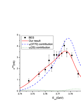
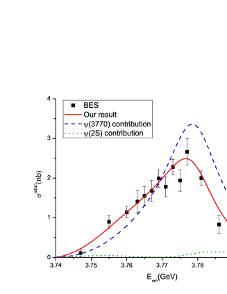
Figure 4: The observed cross sections for $e^{+}e^{-}\rightarrow D^{0}\bar{D}^{0}$ (left plot) and $e^{+}e^{-}\rightarrow D^{+}D^{-}$ (right plot) with $\mu=\delta$. The solid line is the fitting result in our approach shown in Fig.3, the dashed line shows the contribution from Fig.3.(a), and the dotted line shows the contribution from Fig.3.(b). The data are from BES[2].

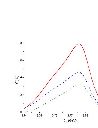
Figure 5: The Born cross section $\sigma^{B}(s)$ for $e^{+}e^{-}\rightarrow D\bar{D}$ with $\mu=\delta$. The solid line is for $e^{+}e^{-}\rightarrow D\bar{D}$, the dashed line is for $e^{+}e^{-}\rightarrow D^{0}\bar{D}^{0}$, and the dotted line is for $e^{+}e^{-}\rightarrow D^{+}D^{-}$.

In summary, we have proposed an effective field theory for low-energy $D\bar{D}$ interactions in which we have included the resonance $\psi(3770)$ and an additional small scale $\delta$. It is found that the coefficient of the contact term $f_{1}$ will be enhanced to be $\mathcal{O}(p^{-2})$. Therefore, the leading $D\bar{D}$ interaction potential in this specific channel would come from the $S$-channel $\psi(3770)$ exchange and the contact term $f_{1}$. With the leading $D\bar{D}$ potential, we then sum the bubble diagrams to describe the $D\bar{D}$ final-state interaction as shown in Fig. 3. We find that we can describe the anomalous cross-section lineshape of $e^{+}e^{-}\to D\bar{D}$ observed by the BESII Collaboration [2] using the effective field theory. This approach should be useful for our further understanding of the $\psi(3770)$ non-$D\bar{D}$ decays, which could share the same dynamic origin as the $D\bar{D}$ cross-section lineshape anomaly as emphasized in Refs. [23, 25].

We also test the effects of the contact term $f_{1}$ and find that, without this term, the extracted value of $g_{\psi(2S)D\bar{D}}$ is too large to make the fitting self-consistent. Nevertheless, the fitted $\psi(3770)$ mass is significantly larger than that in PDG [17, 1]. Our study also suggests that the subthreshold $\psi(2S)$ plays an important role in our understanding of the $D\bar{D}$ interactions. A better determination of $g_{\psi(2S)D\bar{D}}$ should be strongly encouraged.

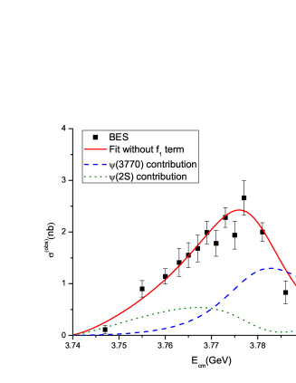
Figure 6: The observed cross sections for $e^{+}e^{-}\rightarrow D^{0}\bar{D}^{0}$ (left plot) and $e^{+}e^{-}\rightarrow D^{+}D^{-}$ (right plot). The solid line is the fitting result with $f_{1}=0,$ and $\mu=0$, the dashed line shows the contribution from $\psi(3770)$, and the dotted line shows the contribution from $\psi(2S)$. The data are from BES [2].

References

[1]
J. Beringer et al.(Particle Data Group), Phys. Rev.
D 86(2012),010001.
[2]
M. Ablikim, et al., BES collaboration, Phys.Lett.B 668(2008)
263.
[3]
Y.J. Zhang and Q. Zhao, Phys.Rev.D 81(2010) 034011.
[8]
G.Y. Chen and J.P. Ma, Phys.Rev.D 83(2011) 094029.
[9]
A. Sibirtsev, J. Haidenbauer, S. Krewald, U. Meißner and A.W. Thomas, Phys. Rev. D 71 (2005) 054010.
[10] J. Haidenbauer, H.-W. Hammer, U. Meissner and A. Sibirtsev, Phys. Lett. B 643 (2006) 29.
[11]
D.B. Kaplan, Nucl.Phys.B 494(1997) 471
[12]
S. Leupold and C. Terschlüsen
arXiv:hep-ph/1206.2253
[13]
T. Bauer and D. R. Yennie, Phys.Lett.B 60(1976), 169.
[14]
G. Li, Q. Zhao and B.S. Zou, Phys.Rev.D 77(2008),014010.
[15]
D.B. Kaplan, M.J. Savage and M.B. Wise, Phys. Lett. B424(1998),390; Nucl.Phys. B 534(1998),329.
[16]
B.W. Long and C.J. Yang, Phys.Rev.C 84(2011), 057001.
[17]
K. Nakamura et al.(Particle Data Group), J. Phys. G: Nucl.
Part. Phys. 37(2010),075021.
[18]
M. Ablikim et al.(BES Collaboration), Phys. Lett.
B603(2004),130;
E.A. Kuraev, V.S. Fadin, Sov. J. Nucl. Phys. 41(1985), 466;
G. Altarelli, G. Martinelli, CERN Yellow Report
86-02(1986), 47;
O. Nicrosini, L. Trentadue, Phys. Lett. B 196(1987), 551.
[19]
D. Besson et al., Phys.Rev.Lett. 96(2006), 092002.
[20]
M.Ablikim et al., BES Collaboration, Phys. Lett.
B 641(2006),145;
M.Ablikim et at., BES Collaboration, Phys. Rev.
Lett 97(2006), 121801;
M.Ablikim et al., BES Collaboration, Phys. Rev.D 76(2007),
122002.
[21]
V. V. Anashin, V. M. Aulchenko, E. M. Baldin, A. K. Barladyan, A. Y. .Barnyakov, M. Y. .Barnyakov, S. E. Baru and I. Y. .Basok et al.,
Phys. Lett. B 711(2012), 292 [arXiv:1109.4205 [hep-ex]].
[22]
Z.G. He, Y. Fan and K.T. Chao, Phys.Rev. Lett. 101(2008),
112001.
[23]
Y. J. Zhang, G. Li and Q. Zhao,
Phys. Rev. Lett. 102 (2009) 172001
[arXiv:0902.1300 [hep-ph]].
[24]
X. Liu, B. Zhang and X. Q. Li,
Phys. Lett. B 675(2009), 441
[arXiv:0902.0480 [hep-ph]].