Nonlinear microrheology of dense colloidal suspensions: a mode-coupling theory

Abstract

A mode-coupling theory for the motion of a strongly forced probe particle in a dense colloidal suspension is presented. Starting point is the Smoluchowski equation for $N$ bath and a single probe particle. The probe performs Brownian motion under the influence of a strong constant and uniform external force $F_{\rm ex}$. It is immersed in a dense homogeneous bath of (different) particles also performing Brownian motion. Fluid and glass states are considered; solvent flow effects are neglected. Based on a formally exact generalized Green-Kubo relation, mode coupling approximations are performed and an integration through transients approach applied. A microscopic theory for the nonlinear velocity-force relations of the probe particle in a dense fluid and for the (de-) localized probe in a glass is obtained. It extends the mode coupling theory of the glass transition to strongly forced tracer motion and describes active microrheology experiments. A force threshold is identified which needs to be overcome to pull the probe particle free in a glass. For the model of hard sphere particles, the microscopic equations for the threshold force and the probability density of the localized probe are solved numerically. Neglecting the spatial structure of the theory, a schematic model is derived which contains two types of bifurcation, the glass transition and the force-induced delocalization, and which allows for analytical and numerical solutions. We discuss its phase diagram, forcing effects on the time-dependent correlation functions, and the friction increment. The model was successfully applied to simulations and experiments on colloidal hard sphere systems [I. Gazuz et. al., Phys. Rev. Lett. 102, 248302 (2009)], while we provide detailed information on its derivation and general properties.

I Introduction

Complex fluids are very common in technological applications as well as in living systems. Rheology Larson (1999) can provide deep insight into their mechanical properties, since it studies their flow and deformation under external force fields. While in conventional macrorheology Waigh (2005); Squires and Mason (2010) mechanical experiments in the bulk are performed, in microrheology the diffusive motion of an embedded, mesoscopic tracer particle is observed. Microrheology thus has an advantage that also materials can be studied, which are not available in large amounts. Corresponding experimental techniques were developed during the last years MacKintosh and Schmidt (1999); Gisler and Weitz (1998); Gittes et al. (1997); Crocker et al. (2000). They utilize the fluctuation-dissipation theorem Forster (1975), which connects the linear response of an observable to external fields with the corresponding time-dependent equilibrium correlation function.

To probe the nonlinear properties of the material in a microrheological experiment, the tracer has to be actively pulled by means of an external force. Corresponding experiments use magnetic forces Habdas et al. (2004); Bausch et al. (1999) as well as optical tweezers Furst (2003); Meyer et al. (2006); Wilson et al. (2009) and measure the nonlinear dependence of the probe velocity on the pulling force.

A typical and ubiquitous nonlinear effect in complex fluids is thinning, i. e. the decay of the tracer friction coefficient with increasing external force. The theoretical understanding of the thinning effect in microrheology was achieved for the case of dilute colloidal suspensions Squires and Brady (2005) by solving the corresponding two-particle diffusion equation. The results of the theory are in good agreement with the simulations Carpen and Brady (2005) and experiments Furst (2003). At larger densities the rheological properties become more complex. If the density exceeds a certain critical value, many complex fluids go in to a disordered solid state and exhibit elastic response Liu and Nagel (1998). In this state, yielding is observed, i. e. the external field must overcome a finite threshold Hastings et al. (2003); Olson Reichhardt and Reichhardt (2010); Fiege et al. (2012) in order to produce a flow. Dense polydisperse colloidal suspensions Hunter and Weeks (2012) represent one of the simplest model system for such viscoelastic complex fluids. Here, neither an exact solution of the underlying many-particle diffusion equation can be given nor perturbative methods can be applied. The mode-coupling theory (MCT) proved to be the method of choice for such systems, since it describes the localization of the tracer in the cage of its nearest neighbours Götze (2009) by accounting for the nonlinear backflow effect in a self-consistent manner.

Recently, a generalization of the standard (quiescent) MCT for the case of nonlinearly pulled tracer was announced Gazuz (2008); Gazuz et al. (2009). The new theory adopts and develops the ideas of the “integration through transients” approach to macrorheology Fuchs and Cates (2002, 2009); Brader et al. (2012) for the case of microrheology. The force-dependent probability density of a localized probe exhibits a bifurcation transition, thus accounting for the yielding effect. For the tracer friction coefficient (in the fluid state or above the yielding threshold in the jammed state), thinning behaviour is observed. In Gazuz et al. (2009), the nonlinear probe velocity-force relations of the schematic model were compared to experiments and simulations. Including fluctuations perpendicular to the forcing directions, the schematic model was extended in Gnann et al. (2011), and discussed in detail in Gnann and Voigtmann (2012) The latter model also could be extended Harrer et al. (2012a) to predict force-induced diffusion Winter et al. (2012) parallel and perpendicular to the external force, based on the microscopic memory kernels which we derive here. The low-force dependence of the tracer probability density was studied in detail Harrer et al. (2012b).

While the above-mentioned recent publications focused on comparison of the theory with experiments and simulations Gazuz et al. (2009); Gnann et al. (2011) and on some of its special aspects Harrer et al. (2012b) and extensions Harrer et al. (2012a); Gnann and Voigtmann (2012), the present paper is intended to provide a comprehensive account of the basics of the theory. We provide the details necessary to understand the derivation of the basic equations and discuss their general properties. Numerical solutions of the MCT equations and (if available) analytical results are presented and compared with each other for both the microscopic version of the theory as well as for the simplified schematic models. For the schematic model, we restrict ourself to the simplest version (where only fluctuations in the force direction are included) and present its explicit derivation from the microscopic theory. Then we discuss the long-time limit, the time dependence of the correlators including the asymptotic results and scaling laws at the vicinity of the critical point as well as the resulting friction coefficient in detail. Also, a version of the schematic model (the “F1-model”) for immobile bath particles is presented, which has not been considered before. The results here are of technical interest (since the equations are simpler and allow analytical solutions), but might be also of interest in connection with the localization transition in the Lorentz model Höfling et al. (2006), which considers a tagged particle in an array of immobile scatterers.

The paper is organized as follows. In Sec. II, the generalized Green-Kubo relation is derived, valid for the nonlinear response to the external force on the tracer. From this general relation, we derive the expression for the tracer friction coefficient. The time-dependent transient tracer density correlators (being the central quantities in our mode-coupling approach) are then introduced and the mode-coupling equations for them as well as the mode-coupling approximation for the tracer friction coefficient are derived. Sec. III presents results for the hard-sphere system. First, the low-density limit of our theory is studied and compared with the exact theory Squires and Brady (2005). Then, the bifurcation transition for the long time limit of the tracer density correlator is studied in detail. Sec. IV, is devoted to the schematic models.

II Theory

II.1 Basic microscopic equations

The Smoluchowski equation will provide the basis for all the considerations in this article:

$$\ \partial_{t}\Psi=\Omega\Psi,$$ (1)

where $\Omega$ is the Smoluchowski operator. Eq. (1) describes the time evolution of the $(N+1)$-particle configuration space probability density $\Psi({\bf r}_{1},\,\ldots,{\bf r}_{N},{\bf r}_{s},t)$ on a coarse-grained time scale, i.e. it is assumed that the velocity fluctuations relax much faster than the configurations. The particles are colloids performing Brownian motion with diffusion coefficients $D_{i}$ in a Newtonian solvent. The particle diffusion coefficients obey the the Stokes-Einstein relation

$$D_{i}=\frac{k_{B}T}{6\pi\eta\,a_{i}},$$ (2)

where $\eta$ is the solvent viscosity and $a_{i}$ the radius of particle $i$. The colloids are allowed to interact by means of the potential forces ${\bf F}_{i}=-\mbox{\boldmath$\partial$}_{i}V({\bf r}_{1},\,\ldots,{\bf r}_{N})$ ($\mbox{\boldmath$\partial$}_{i}$ denotes the partial derivative $\partial/\partial{\mathbf{r}}_{i}$), whereas the hydrodynamic interactions will be neglected.

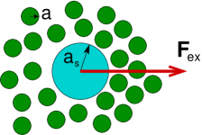
Figure 1: (Color online). The colloidal “tracer” particle is pulled through the suspension of “bath” particles by means of the external force ${\bf F}_{ex}$. The tracer radius is $a_{s}$, and a bath particle has radius $a$.

We consider a single, distinguished particle (the “tracer”) with position ${\bf r}_{s}$ and the diffusion coefficient $D_{s}$ surrounded by $N$ identical particles (the “bath”), which have the diffusion coefficient $D_{0}$. The tracer is pulled by means of the external force ${\bf F}_{ex}$ (see Fig. 1) through the suspension. The full Smoluchowski operator

$$\Omega=\Omega_{0}+\Delta\Omega$$ (3)

consists of the unperturbed part

$$\Omega_{0}=D_{0}\sum_{i=1,\,\ldots,N}\mbox{\boldmath$\partial$}_{i}\cdot(\mbox{\boldmath$\partial$}_{i}-\frac{1}{k_{B}T}{\bf F}_{i})+D_{s}\mbox{\boldmath$\partial$}_{s}\cdot(\mbox{\boldmath$\partial$}_{s}-\frac{1}{k_{B}T}{\bf F}_{s})$$ (4)

and the perturbation due to ${\bf F}_{\rm ex}$

$$\Delta\Omega=-\frac{D_{s}}{k_{B}T}{\bf F}_{ex}\cdot\mbox{\boldmath$\partial$}_{s}.$$ (5)

${\bf F}_{ex}$ will be assumed to be constant in space and time. From now on, we set $k_{B}T=1$ in the Smoluchowski operator to simplify the notation. For comparisons with experiments or simulations, the factor $k_{B}T$ will be reintroduced.

In the following, equilibrium-weighted averages $\int d\Gamma\Psi_{eq}\,\ldots$ will appear, which will be denoted by $\langle\ldots\rangle$, where

$$\Psi_{eq}=\frac{1}{Z}\,e^{-V(\{{\bf r}_{i}\},{\bf r}_{s})}$$ (6)

is the equilibrium distribution of the unperturbed system with the statistical sum $Z$. We also introduce the usual equilibrium-weighted scalar product, which is defined as

$$\langle A\,|B\rangle=\int d\Gamma\Psi_{eq}\,A^{*}(\Gamma)B(\Gamma)$$ (7)

for two configuration-space observables $A$ and $B$.

II.2 Nonlinear response to the external force on the tracer

Let us consider the following situation. For times $t<0$, the system is equilibrated and there are no external fields. At $t=0$, the external force on the tracer is switched on, driving the system out of equilibrium. Instead of assuming that the perturbation is small, like it is done in the linear response theory, we consider the general case of arbitrarily large forces.

With the initial condition

$$\Psi(t=0)=\Psi_{eq},$$ (8)

the solution of the Smoluchowski equation can be written down as

$$\Psi(t)=e^{\Omega\,t}\,\Psi_{eq}$$ (9)

Using the operator identity

$$e^{\Omega\,t}=1+\int_{0}^{t}dt^{\prime}\,e^{\Omega\,t^{\prime}}\,\Omega$$ (10)

and noting that $\Omega\Psi_{eq}=\Delta\Omega\Psi_{eq}$, we get

$$\Psi(t)=\Psi_{eq}+\int_{0}^{t}dt^{\prime}\,e^{\Omega\,t^{\prime}}\Delta\Omega\Psi_{eq}$$ (11)

The mean value of an observable $A({\bf r}_{1},\,\ldots,{\bf r}_{N})$ at time $t$ is given by:

$$\langle A(t)\rangle=\int d\Gamma\,\Psi(\Gamma,t)A(\Gamma),$$ (12)

where $\Gamma$ is a phase space point and the integration goes over the entire phase space. Using eq. (11), we obtain

$$\langle A(t)\rangle=\langle A\rangle-D_{s}\int d\Gamma\,A(\Gamma)\int_{0}^{t}dt^{\prime}\,e^{\Omega\,t^{\prime}}({\bf F}_{ex}\cdot\mbox{\boldmath$\partial$}_{s})\,\Psi_{eq}.$$ (13)

We note that $\mbox{\boldmath$\partial$}_{s}\,\Psi_{eq}={\bf F}_{s}\Psi_{eq}$, introduce

$$\Omega^{\dagger}=\Omega_{0}^{\dagger}+\Delta\Omega^{\dagger}\,,$$ (14)

the adjoint of $\Omega$ with respect to the unweighted scalar product Dhont (1996), with

$$\Omega_{0}^{\dagger}=\sum_{i=1}^{N}D_{0}\,(\mbox{\boldmath$\partial$}_{i}+{\bf F}_{i})\cdot\mbox{\boldmath$\partial$}_{i}+D_{s}\,(\mbox{\boldmath$\partial$}_{s}+{\bf F}_{s})\cdot\mbox{\boldmath$\partial$}_{s}$$ (15)

and $\Delta\Omega^{\dagger}=D_{s}\,{\bf F}_{ex}\cdot\mbox{\boldmath$\partial$}_{s}$, and finally arrive at

$$\langle A\rangle(t)=\langle A\rangle-D_{s}\,{\bf F}_{ex}\cdot\int_{0}^{t}dt^{\prime}\,\langle\,{\bf F}_{s}\,e^{\Omega^{\dagger}\,t^{\prime}}A\,\rangle\,.$$ (16)

Eq. (16) represents the generalized nonlinear Green-Kubo relation for the response of an observable $A$ to the perturbation by the external force on the tracer. In contrast to the well-known linear response expression, the full Smoluchowski operator $\Omega$ containing the external force, instead of just the unperturbed one enters eq. (16).

The presence of an external force renders the operator (14) nonhermitian with respect to the equilibrium-weighted scalar product (7). Its adjoint is now given by

$$\Omega^{adj}=\Omega^{\dagger}_{0}-D_{s}\,{\bf F}_{ex}\cdot({\bf F}_{s}+\mbox{\boldmath$\partial$}_{s})$$ (17)

(the calculation is presented in Gazuz (2008)).

II.3 Tracer mobility

The (long-time) tracer mobility is defined as

$$\mu_{s}=\lim_{t\rightarrow\infty}\frac{\langle{\bf v}_{s}\rangle(t)}{{\bf F}_{ex}},$$ (18)

where ${\bf v}_{s}$ is the tracer velocity. In the framework of the Smoluchowski dynamics, where the particle motion is overdamped, the tracer velocity ${\bf v}_{s}=\partial_{t}{\bf r}_{s}=\Omega^{\dagger}{\bf r}_{s}$ is a function on the configurational space and is given by

$${\bf v}_{s}=\mu_{s}^{0}({\bf F}_{ex}+{\bf F}_{s}),$$ (19)

where $\mu_{s}^{0}=D_{s}/(k_{B}T)$ is the single-particle tracer mobility. Since ${\bf F}_{ex}$ is given externally and has no dependence on the phase space of the system, the problem reduces to calculating the average of the force ${\bf F}_{s}$ from the bath particles on the tracer. To determine $\langle F^{\alpha}_{s}\rangle$, the $\alpha$-th component of the vector $\langle{\bf F}_{s}\rangle$, we use eq. (16), note that the equilibrium average $\langle{\bf F}_{s}\rangle$ vanishes and obtain

$$\langle F^{\alpha}_{s}\rangle(t)=-D_{s}{\bf F}_{ex}\int_{0}^{t}dt^{\prime}\,\langle{\bf F}_{s}\,e^{\Omega^{\dagger}\,t^{\prime}}F^{\alpha}_{s}\rangle\,.$$ (20)

Let us introduce the coordinate system such that ${\bf F}_{\rm ex}$ points in the positive $z$-direction. Then we have ${\bf F}_{\rm ex}\cdot{\bf F}^{s}=F_{ex}F^{z}_{s}$ in eq. (20). Expression (20) can be simplified further if we employ the rotation symmetry around the $z$-axis, which our system obviously exhibits. After such a rotation, the phase space integral in (20) should remain the same. On the other hand, rotations by angle $\pi$ change the sign of both the $x$- and the $y$-component of ${\bf F}^{s}$. This means that the correlators $\langle F^{z}_{s}\,e^{\Omega^{\dagger}\,t^{\prime}}F^{x}_{s}\rangle$ and $\langle F^{z}_{s}\,e^{\Omega^{\dagger}\,t^{\prime}}F^{y}_{s}\rangle$ vanish and we are left with

$$\langle{\bf F}_{s}\rangle(t)=-D_{s}{\bf F}_{ex}\int_{0}^{t}dt^{\prime}\,\langle{F^{z}_{s}}\,e^{\Omega^{\dagger}\,t^{\prime}}{F^{z}_{s}}\rangle\,.$$ (21)

As was anticipated in eq. (18), the mean force exerted from the bath on the tracer is parallel to the external force ${\bf F}_{\rm ex}$.

Expression (21) includes the force-force correlator $C(t)=\langle{F^{z}_{s}}\,e^{\Omega^{\dagger}\,t^{\prime}}{F^{z}_{s}}\rangle$ and leads for the tracer mobility to the result

$$\mu_{s}=\mu_{s}^{0}\left(1-D_{s}\int_{0}^{\infty}dt\,C(t)\right).$$ (22)

For the further use together with the mode-coupling approximations, the force-force correlator in eq. (22) should be rewritten in terms of the irreducible Smoluchowski operator

$$\Omega^{\dagger\,\mbox{\tiny irr}}=\Omega^{\dagger}-{F^{z}_{s}}\rangle D_{s}^{-1}\langle{F^{z}_{s}},$$ (23)

following Cichocki and Hess (1987); Kawasaki (1995). After changing to the Laplace space according to $C(z)=\int_{0}^{\infty}dt\,e^{-zt}C(t)$,

$$C(z)=\langle{F^{z}_{s}}\frac{1}{z-\Omega^{\dagger}}{F^{z}_{s}}\rangle$$ (24)

and using the standard operator identity for $A=A_{1}+A_{2}$

$$(z-A)^{-1}=(z-A_{1})^{-1}+(z-A)^{-1}A_{2}(z-A_{1})^{-1},$$ (25)

(with $A=\Omega^{\dagger}$, $A_{1}=\Omega^{\dagger\,\mbox{\tiny irr}}$) for the resolvent in (24), one obtains the expression

$$C(z)=\frac{C^{\mbox{\tiny irr}}(z)}{1+D_{s}C^{\mbox{\tiny irr}}(z)}$$ (26)

for the force-force correlator in terms of the irreducible one $C^{\mbox{\tiny irr}}(z)=\langle{F^{z}_{s}}\,(z-\Omega^{\dagger\,\mbox{\tiny irr}})^{-1}{F^{z}_{s}}\rangle$. Exploiting the relation (26) for $z=0$ leads us to the desired result

$$\mu_{s}=\frac{\mu_{s}^{0}}{1+D_{s}\int_{0}^{\infty}dt\,C^{\mbox{\tiny irr}}(t)}$$ (27)

for the tracer mobility in terms of the irreducible tracer force autocorrelation function $C^{\mbox{\tiny irr}}(t)$, which in the time domain is given by

$$C^{\mbox{\tiny irr}}(t)=\langle{F^{z}_{s}}\,e^{\Omega^{\dagger\,\mbox{\tiny irr}}\,t}{F^{z}_{s}}\rangle$$ (28)

Eq. (27) allows a simple interpretation if one introduces the tracer friction coefficient $\zeta_{s}=1/\mu_{s}$. The friction coefficient is given by the sum

$$\zeta_{s} = \zeta_{s}^{0}+\Delta\zeta_{s},$$ (29)

$$\Delta\zeta_{s} = \int_{0}^{\infty}dt\,C^{\mbox{\tiny irr}}(t),$$ (30)

of the “bare” (single-particle) tracer friction coefficient due to the solvent, given by $\zeta_{s}^{0}=1/\mu_{s}^{0}$ and the increment $\Delta\zeta_{s}$ due to interactions with the bath particles. Because we are interested in dense dispersions where the friction is highly increased beyond the solvent one, Eq. (29) provides a more secure route to approximations than Eq. (22). In Eq. (29) slow force fluctuations contribute to an increased friction. In Eq. (22), instantaneous and retarded velocity fluctuations need to cancel in order to yield a reduced mobility. The mode coupling approximations to be performed later set up a self-consistent set of equations for slow fluctuations which is better tailored to Eq. (29) than to Eq. (22). Recent simulations of a forced probe in a bath of noninteracting bath particles support to approximate $C^{\mbox{\tiny irr}}$ instead of $C$ Zia and Brady (2010). Even though the bath particles do not interact among themselves, the collisions with the probe particle induce correlations in the velocity but not (or to lesser extent) in the force fluctuations. The friction increment increases linearly with bath density, as expected from independent collisions of the non-interacting bath particles with the probe. This expected behavior, however, does not hold for the mobility change, which varies more rapidly with bath density Zia and Brady (2010).

After these formally exact manipulations, approximations are now required in order to evaluate the irreducible force correlation function. Low density approximations have been performed Squires and Brady (2005), and we will use mode coupling approximations to address high packing fractions close to the colloidal glass transition.

II.4 Transient tracer density fluctuations

The important quantities in the mode-coupling approach are the tracer and the bath densities

$$\rho^{s}({\bf r}) = \delta({\bf r}-{\bf r}_{s}),$$ (31)

$$\rho({\bf r}) = \sum_{i=1}^{N}\delta({\bf r}-{\bf r}_{i}).$$ (32)

With the convention for the Fourier transform of a function $X({\bf r})$ to be

$$X({\bf q})=\int d{\bf r}\,e^{i\,{\bf q}\cdot{\bf r}}\,X({\bf r}),$$ (33)

implying

$$X({\bf r})=\frac{1}{(2\pi)^{3}}\int d{\bf q}\,e^{-i\,{\bf q}\cdot{\bf r}}\,X({\bf q})$$ (34)

for the back-transform, we have

$$\rho^{s}_{\bf q} = e^{i\,{\bf q}\cdot{\bf r}_{s}}$$ (35)

$$\rho_{\bf q} = \sum_{i=1}^{N}e^{i\,{\bf q}\cdot{\bf r}_{i}}.$$ (36)

for the tracer and the bath density modes.

II.4.1 General properties

The first question to clarify concerns the time-dependent correlator

$$\langle\rho^{s}_{\bf q}e^{\Omega^{\dagger}\,t}\rho^{s}_{{\bf q}^{\prime}}\rangle$$ (37)

of two tracer density modes. For which pairs of wavevectors ${\bf q}$, ${\bf q}^{\prime}$ is it nonzero ?

For the case of an isolated system, translational invariance implies that after all particle positions have been shifted

$$\Gamma\rightarrow\Gamma^{\prime}$$ (38)

with ${\bf r}_{s}\rightarrow{\bf r}_{s}+{\bf a}$, ${\bf r}_{i}\rightarrow{\bf r}_{i}+{\bf a}$ ($i=1,\ldots,\,N$), the average (37) should remain the same. Since the shift introduces the prefactor $e^{i\,({\bf q}+{\bf q}^{\prime})\cdot{\bf a}}$ in eq. (37) and the vector ${\bf a}$ can be arbitrary, the condition

$${\bf q}=-{\bf q}^{\prime}$$ (39)

follows.

Our driven system is translationally invariant as well, since we assume the external force ${\bf F}_{ex}$ to be space and time independent and the Smoluchowski operator (14) does not change after the shift (38). Thus, the argumentation used for the isolated systems and thus the condition (39) remains.

We can thus introduce the usual notation

$$\phi^{s}_{\bf q}(t) = \langle\rho^{s*}_{\bf q}e^{\Omega^{\dagger}\,t}\rho^{s}_{{\bf q}}\rangle,$$ (40)

$$\phi_{\bf q}(t) = \frac{1}{NS_{q}}\langle\rho^{*}_{\bf q}e^{\Omega^{\dagger}\,t}\rho_{{\bf q}}\rangle\,$$ (41)

for the tracer and the bath density mode correlators, where $S_{q}$ is the bath static structure factor

$$S_{q}=\frac{1}{N}\,\langle\rho^{*}_{{\bf q}}\,\rho_{\bf q}\rangle.$$ (42)

The Fourier back transform of $\phi^{s}_{\bf q}(t)$:

$$\phi^{s}({\bf r})(t)=FT^{-1}[\phi^{s}_{\bf q}(t)].$$ (43)

is the probability density of finding the tracer at the point ${\bf r}$ in space at time $t$ with the initial condition that at time $t=0$ it was localized at the origin. The derivation is given in Ref. Hess and Klein (1983), where an isolated system is considered. Since no special properties of the Smoluchowski operator for isolated systems are used in Ref. Hess and Klein (1983), the derivation is valid also for our case.

The general condition for the Fourier back transform (43) to be real is

$$\phi^{s}_{-{\bf q}}(t)=\phi^{s\,*}_{\bf q}(t).$$ (44)

We can easily see that the property (44) is indeed fulfilled by $\phi^{s}_{\bf q}$ if we use it’s definition (40) and the fact that the operator $e^{\Omega^{\dagger}\,t}$ is linear and real (since it contains derivatives with respect to phase space coordinates multiplied by real numbers). So,

$$\phi^{s\,*}_{\bf q}(t)=\langle\left(e^{i\,{\bf q}\cdot{\bf r}_{s}}\,e^{\Omega^{\dagger}\,t}\,e^{-i\,{\bf q}\cdot{\bf r}_{s}}\right)^{*}\rangle=\quad\quad\quad\quad$$

$$=\langle e^{-i\,{\bf q}\cdot{\bf r}_{s}}\,e^{\Omega^{\dagger}\,t}\,e^{i\,{\bf q}\cdot{\bf r}_{s}}\rangle=\phi^{s}_{-\bf q}(t)$$ (45)

II.4.2 Zwanzig-Mori equations

The Zwanzig-Mori projector operator formalism allows one to express the fluctuations of a given observable in terms of the corresponding memory kernel. After introducing the projectors $P_{A}=A\rangle\langle A^{*}$, $Q_{A}=1-P_{A}$ for an observable $A$ (we assume that $\langle A^{*}A\rangle=1$ for simplicity), the Laplace transform $C(z)=\int_{0}^{\infty}dt\,e^{-zt}C_{A}(t)$ of its equilibrium time correlation function $C_{A}(t)=\langle A^{*}e^{\Omega^{\dagger}\,t}A\rangle$ can be written as Forster (1975)

$$C_{A}(z)=\frac{1}{z+\omega_{A}-M_{A}(z)},$$ (46)

where the frequency $E_{A}$ and the memory function $M_{A}(z)$ are given by

$$\omega_{A} = -\langle A^{*}\Omega^{\dagger}A\rangle,$$ (47)

$$M_{A}(z) = \langle A^{*}\Omega^{\dagger}\,Q_{A}\frac{1}{z-Q_{A}\Omega^{\dagger}Q_{A}}Q_{A}\Omega^{\dagger}A\rangle.$$ (48)

In the time domain, eq. (46) corresponds to

$$\partial_{t}\,C_{A}(t)=-\omega_{A}\,C_{A}(t)+\int_{0}^{t}dt^{\prime}M_{A}(t-t^{\prime})\,C_{A}(t^{\prime}).$$ (49)

For dissipative systems, like for the case of our system described by the Smoluchowski operator, a second projection step is needed Cichocki and Hess (1987); Kawasaki (1995). To this end, one introduces the irreducible Smoluchowski operator

$$\Omega^{\dagger\,\mbox{\tiny irr}}=Q_{A}\left(\Omega^{\dagger}-\Omega^{\dagger}A\rangle\langle A^{*}\Omega^{\dagger}A\rangle^{-1}\langle A^{*}\Omega^{\dagger}\,\right)Q_{A}.$$ (50)

and gets the representation

$$M_{A}(z)=\frac{M^{\mbox{\tiny irr}}_{A}(z)}{1+\omega_{A}^{-1}M^{\mbox{\tiny irr}}_{A}(z)}$$ (51)

for the memory function in terms of the irreducible memory function $M^{\mbox{\tiny irr}}_{A}(z)$ given by

$$M^{\mbox{\tiny irr}}_{A}(z)=\langle A^{*}\Omega^{\dagger}\,Q_{A}\frac{1}{z-\Omega^{\dagger\,\mbox{\tiny irr}}}Q_{A}\Omega^{\dagger}A\rangle,$$ (52)

which time evolution is generated by $\Omega^{\dagger\,\mbox{\tiny irr}}$: $M^{\mbox{\tiny irr}}_{A}(t)=\langle A^{*}\Omega^{\dagger}\,Q_{A}e^{\Omega^{\dagger\,\mbox{\tiny irr}}t}Q_{A}\Omega^{\dagger}A\rangle$. For the irreducible memory equation, one obtains in the time domain

$$\partial_{t}\,C_{A}(t)=-\omega_{A}\,C_{A}(t)-\frac{1}{\omega_{A}}\int_{0}^{t}dt^{\prime}M^{\mbox{\tiny irr}}_{A}(t-t^{\prime})\,\partial_{t}^{\prime}\,C_{A}(t^{\prime}).$$ (53)

The procedure of expressing the equilibrium correlation functions in terms of memory kernels sketched above, was originally proposed for an isolated system evolving with the unperturbed operator $\Omega^{\dagger}_{0}$. We apply it to the correlators evolving with the nonhermitian operator $\Omega^{\dagger}$ even though the mathematical conditions and justifications are unknown at present. This procedure is based on the conjecture that the algebraic structure of the Zwanzig-Mori equations together with the mode coupling approximations, necessary in the latter steps to evaluate them, capture the mathematical bifurcation describing the delocalization of the probe under strong force. At present this conjecture can only be tested by formulating the theory and considering its results in comparisons with data and formal symmetry requirements.

After these considerations, we are in a position to write down the memory equation for $\phi^{s}_{\bf q}(t)=\langle\rho^{s*}_{\bf q}e^{\Omega^{\dagger}\,t}\rho^{s}_{{\bf q}}\rangle$:

$$\partial_{t}\,\phi^{s}_{\bf q}(t)=-\omega_{\bf q}\,\phi^{s}_{\bf q}(t)-\frac{1}{\omega_{\bf q}}\int_{0}^{t}dt^{\prime}M^{s,\mbox{\tiny irr}}_{\bf q}(t-t^{\prime})\,\partial_{t^{\prime}}{\phi}^{s}_{\bf q}(t^{\prime}),$$ (54)

with

$$\omega_{\bf q} = -\langle\rho^{s*}_{\bf q}\,\Omega^{\dagger}\,\rho^{s}_{\bf q}\rangle,$$ (55)

$$M^{s,\mbox{\tiny irr}}_{\bf q}(t) = \langle\rho^{s*}_{\bf q}\,\Omega^{\dagger}\,Q^{s}\,e^{\Omega^{\dagger\,\mbox{\tiny irr}}t}\,Q^{s}\,\Omega^{\dagger}\,\rho^{s}_{\bf q}\rangle$$ (56)

$$\Omega^{\dagger\,\mbox{\tiny irr}} = Q^{s}\left(\Omega^{\dagger}-\Omega^{\dagger}\,\rho^{s}_{\bf q}\rangle\,\omega_{\bf q}^{-1}\langle\rho^{s*}_{\bf q}\,\Omega^{\dagger}\,\right)Q^{s}$$ (57)

and the projector

$$Q^{s}=1-\rho^{s}_{\bf q}\rangle\langle\rho^{s*}_{\bf q}\,.$$ (58)

Applying $\Omega^{\dagger}$ to $\rho^{s}_{\bf q}$ yields

$$\Omega^{\dagger}\,\rho^{s}_{\bf q}=D_{s}\,(\mbox{\boldmath$\partial$}_{s}^{2}+({\bf F}_{s}+{\bf F}_{ex})\cdot\mbox{\boldmath$\partial$}_{s})\,e^{i\,{\bf q}\cdot{\bf r}_{s}}\quad\quad$$ (59)

$$=D_{s}\,(-q^{2}+i\,{\bf q}\cdot({\bf F}_{s}+{\bf F}_{ex}))\,\rho^{s}_{\bf q}\,,$$

so for the frequency $\omega_{\bf q}$ we obtain

$$\omega_{\bf q}=D_{s}\,(q^{2}-i\,{\bf q}\cdot{\bf F}_{ex}).$$ (60)

The fact that $\omega_{\bf q}=-\langle\rho^{s}_{\bf q}\,|\,\Omega^{\dagger}\,|\,\rho^{s}_{\bf q}\rangle$ turns out to be complex is obviously the consequence of the mentioned nonhermiticity of the operator $\Omega^{\dagger}=\Omega^{\dagger}_{0}+D_{s}\,{\bf F}_{ex}\cdot\mbox{\boldmath$\partial$}_{s}$ with respect to the equilibrium-weighted scalar product (7).

We would like to discuss now the relationship between the irreducible operator introduced in eq. (23) for the force-force correlator (call it $\Omega^{\dagger\,\mbox{\tiny irr}}({F^{z}_{s}})$) and the one introduced in eq. (57) for the tracer density modes (call it $\Omega^{\dagger\,\mbox{\tiny irr}}(\rho^{s}_{\bf q})$). To this end, we set ${\bf F}_{\rm ex}=0$, go to the limit ${\bf q}\rightarrow 0$ in eq. (57) and employ relations (59), (60). Then, we readily see that

$$\lim_{{\bf q}\rightarrow 0}\Omega^{\dagger\,\mbox{\tiny irr}}(\rho^{s}_{\bf q})=\Omega^{\dagger\,\mbox{\tiny irr}}({F^{z}_{s}})\quad(\mbox{at}\ \ F_{\rm ex}=0)$$ (61)

holds. It is not surprising, since the $({\bf q}\rightarrow 0,z\rightarrow 0)$ limit for the tracer density fluctuations is related to the tracer diffusion and in the absence of the external force, the well-known relation Nägele and Dhont (1998); Fuchs et al. (1998)

$$D^{L}_{s}=\frac{D_{s}}{1+\lim_{{\bf q}\rightarrow 0,z\rightarrow 0}\left(M^{s,\mbox{\tiny irr}}_{\bf q}({\bf q},z)/\omega_{\bf q}\right)}$$ (62)

for the long-time tracer diffusion coefficient $D^{L}_{s}$ implies the Einstein relation

$$D^{L}_{s}=\mu_{s}\quad(\mbox{at}\ \ F_{\rm ex}=0)$$ (63)

connecting $D^{L}_{s}$ with the long time tracer mobility $\mu_{s}$ considered in the last section. We see that the irreducible memory function plays the role of a generalized friction kernel.

II.5 Mode-coupling approximations

II.5.1 The memory function

In order to obtain a self-consistent equation for $\phi^{s}_{\bf q}$ from the memory equation (54), the irreducible memory function (56) is treated using the standard approximation steps of the mode-coupling theory Götze (2009). To this end, first, the projectors onto the space spanned by the tracer-bath density products

$$P^{s}_{2}=\sum_{{\bf k},{\bf p},{\bf k}^{\prime},{\bf p}^{\prime}}\rho^{s}_{\bf k}\rho_{\bf p}\rangle\,g({\bf k},{\bf p},{\bf k}^{\prime},{\bf p}^{\prime})\,\langle\rho^{s*}_{\bf k^{\prime}}\rho^{*}_{\bf p^{\prime}}$$ (64)

are introduced, where the normalization matrix $g$ has to obey the condition

$$\sum_{{\bf k}^{\prime},{\bf p}^{\prime}}\langle\rho^{s}_{\bf k^{\prime}}\rho_{\bf p^{\prime}}\,|\,\rho^{s}_{\bf k}\rho_{\bf p}\rangle\,g({\bf n},{\bf m},{\bf k}^{\prime},{\bf p}^{\prime})=\delta_{{\bf n},{\bf k}}\,\delta_{{\bf m},{\bf p}}$$ (65)

which requires an arbitrary vector $|\,\rho^{s}_{\bf k}\rho_{\bf p}\rangle$ from the space of the tracer and bath density products to be left invariant upon application of $P^{s}_{2}$.

As the first approximation, the “fluctuating forces” $Q^{s}\,\Omega^{\dagger}\,\rho^{s}_{\bf q}$ in eq. (56) are replaced by the projected ones:

$$M^{s,\mbox{\tiny irr}}_{\bf q}\approx\langle\rho^{s*}_{\bf q}\,\Omega^{\dagger}\,Q^{s}\,P^{s}_{2}\,e^{\Omega^{\dagger\,\mbox{\tiny irr}}t}\,P^{s}_{2}\,Q^{s}\,\Omega^{\dagger}\,\rho^{s}_{\bf q}\rangle.$$ (66)

In the next approximation step, the four-point correlators $\langle\rho^{s*}_{\bf k}\rho^{*}_{\bf p}\,e^{\Omega^{\dagger\,\mbox{\tiny irr}}t}\,\rho^{s}_{{\bf k}^{\prime}}\rho_{{\bf p}^{\prime}}\rangle$ appearing in eq. (66) are factorized into products of the two-point ones Götze (1991):

$$\langle\rho^{s*}_{\bf k}\rho^{*}_{\bf p}\,e^{\Omega^{\dagger\,\mbox{\tiny irr}}t}\,\rho^{s}_{{\bf k}^{\prime}}\rho_{{\bf p}^{\prime}}\rangle\quad\quad\quad\quad\quad\quad\quad\quad\quad\quad\quad\quad\quad$$ (67)

$$\approx\delta_{{\bf k},{\bf k}^{\prime}}\,\delta_{{\bf p},{\bf p}^{\prime}}\,\langle\rho^{s*}_{\bf k}e^{\Omega^{\dagger}\,t}\rho^{s}_{{\bf k}^{\prime}}\rangle\,\langle\rho^{*}_{\bf p}e^{\Omega^{\dagger}\,t}\rho_{{\bf p}^{\prime}}\rangle$$

$$=\delta_{{\bf k},{\bf k}^{\prime}}\,\delta_{{\bf p},{\bf p}^{\prime}}\,\phi^{s}_{\bf k}(t)\,NS_{p}\,\phi_{\bf p}(t).$$

Note also that as part of the approximation, the irreducible operator on the left hand side of eq. (67) was replaced by the normal one on the right hand side.

It is easy to see that for $t=0$, the factorization approximation (67) becomes exact and allows us to calculate the normalization matrix $g$ from the condition (65), which then reads

$$\sum_{{\bf k}^{\prime},{\bf p}^{\prime}}\delta_{{\bf k}^{\prime},{\bf k}}\,\delta_{{\bf p}^{\prime},{\bf p}}NS_{p}\,g({\bf n},{\bf m},{\bf k}^{\prime},{\bf p}^{\prime})=\delta_{{\bf n},{\bf k}}\,\delta_{{\bf m},{\bf p}},$$ (68)

leading to the result

$$g({\bf n},{\bf m},{\bf k},{\bf p})=\frac{1}{NS_{p}}\delta_{{\bf n},{\bf k}}\,\delta_{{\bf m},{\bf p}}.$$ (69)

The only missing parts appearing after the application of the projectors $P^{2}_{s}$ in the expression (66) are now the static averages of the form

$$\langle\rho^{s*}_{{\bf k}}\rho^{*}_{{\bf p}}\,Q^{s}\Omega^{\dagger}\rho^{s}_{\bf q}\rangle$$ (70)

and

$$\langle\rho^{s*}_{\bf q}\,\Omega^{\dagger}\,Q^{s}\rho^{s}_{{\bf k}}\rho_{{\bf p}}\rangle.$$ (71)

First, we notice that since $\Omega^{\dagger}$ is not self-adjoint, the averages (70), (71) are not complex conjugated of each other, as it would be the case for an isolated system. Using eqs. (58), (59), for the term (70) we obtain

$$\frac{1}{D_{s}}\langle\rho^{s*}_{\bf k}\rho^{*}_{\bf p}\,Q^{s}\Omega^{\dagger}\rho^{s}_{\bf q}\rangle=\langle\rho^{s}_{\bf q-k}\,\rho^{*}_{\bf p}\,(-q^{2}+i\,{\bf q}\cdot({\bf F}_{s}+{\bf F}_{ex}))\rho^{s}_{\bf q}\rangle$$

$$-\,\langle\rho^{s}_{\bf q-k}\,\rho^{*}_{\bf p}\rangle\,(-q^{2}+i\,{\bf q}\cdot({\bf F}_{s}+{\bf F}_{ex}))\,.\quad\quad\quad\quad$$ (72)

The nontrivial terms in the above expression are either of the form of the tracer-bath static structure factor

$$S^{s}_{p}=\,\langle\rho^{s*}_{\bf p}\,\rho_{{\bf p}}\rangle$$ (73)

or the term of the form $\langle{\bf F}_{s}\,\rho^{s}_{\bf k}\rho_{\bf p}\rangle$. The latter can be reduced to the tracer-bath static structure factor by means of partial integration

$$\langle{\bf F}_{s}\,\rho^{s}_{\bf k}\rho_{\bf p}\rangle=\frac{1}{Z}\int d\Gamma\,(\mbox{\boldmath$\partial$}_{s}e^{-V})\rho^{s}_{\bf k}\rho_{\bf p}=\quad\quad\quad\quad\quad\quad\quad$$

$$=-\frac{1}{Z}\int d\Gamma\,e^{-V}\mbox{\boldmath$\partial$}_{s}(\rho^{s}_{\bf k}\rho_{\bf p})=-i{\bf k}\,\delta_{{\bf k}+{\bf p},0}\,S^{s}_{p}\,.\quad\quad$$ (74)

Using this relation, one readily obtains the result

$$\langle\rho^{s*}_{\bf k}\rho^{*}_{\bf p}\,Q^{s}\Omega^{\dagger}\,\rho^{s}_{\bf q}\rangle=\delta_{{\bf q},\,{\bf k}+{\bf p}}\,D_{s}S^{s}_{p}\,({\bf q}\cdot{\bf p})$$ (75)

To calculate the remaining average (71), the fastest way is to we use the adjoint of $\Omega^{\dagger}$:

$$\langle\rho^{s*}_{\bf q}\,\Omega^{\dagger}Q^{s}\,\rho^{s}_{\bf k}\rho_{\bf p}\rangle=\langle(\Omega^{adj}\rho^{s*}_{\bf q})Q^{s}\,\rho^{s}_{\bf k}\rho_{\bf p}\rangle$$ (76)

and its action on the conjugated tracer density mode (see eq. (17)):

$$\Omega^{adj}\,\rho^{s*}_{\bf q}=D_{s}\,(-q^{2}-i\,{\bf q}\cdot({\bf F}_{s}-{\bf F}_{ex})-{\bf F}_{ex}\cdot{\bf F}_{s})\,\rho^{s*}_{\bf q}.$$ (77)

The calculations go in the same way as for the term (70) and we omit the details except for the fact that compared to the expression (59), an additional term ${\bf F}_{ex}\cdot{\bf F}_{s}$ is present in the brackets in eq. (77), so that the final result also contains ${\bf F}_{\rm ex}$:

$$\langle\rho^{s*}_{\bf q}\,\Omega^{\dagger}Q^{s}\,\rho^{s}_{\bf k}\rho_{\bf p}\rangle=\delta_{{\bf q},\,{\bf k}+{\bf p}}\,D_{s}S^{s}_{p}\,({\bf q}\cdot{\bf p}-i\,{\bf F}_{ex}\cdot{\bf p})\,.$$ (78)

After collecting the terms together, using relations (66), (67), (69), (75) and (78), the final mode-coupling expression for the memory function reads

$$M^{s,\mbox{\tiny irr}}_{\bf q}(t)=\sum_{{\bf k}+{\bf p}=\,{\bf q}}\frac{D^{2}_{s}{S_{p}^{s}}^{2}}{NS_{p}}\,{\bf q}\cdot{\bf p}\left({\bf q}\cdot{\bf p}-i\,{\bf F}_{ex}\cdot{\bf p}\right)\,\phi^{s}_{{\bf k}}(t)\phi_{{\bf p}}(t).$$ (79)

II.5.2 The bulk dynamics

So far, nothing was said about the fluctuations of the bulk density modes $\phi_{{\bf q}}(t)$. The simplest reasonable assumption for these is, to neglect the effect of the external force. In the thermodynamic limit, which is considered in this article, this assumption is justified, since the effect of the tracer on the bath will be to perturb its neighbourhood only locally. This effect will be included in our theory and can be described by the tracer and bath density mode products $\rho^{s}_{\bf q}\rho_{\bf q}$, which are the Fourier space counterparts of the relative bath-tracer density $\rho({\bf r}-{\bf r}_{s})$.

So, we assume the bulk bath dynamics to be unaffected by the external force. The memory equation for the bulk dynamics reads

$$\tau_{q}\,\partial_{t}\phi_{\bf q}(t)+\phi_{\bf q}(t)+\int_{0}^{t}dt^{\prime}\,M^{\mbox{\tiny irr}}_{\bf q}(t-t^{\prime})\,\partial_{t^{\prime}}\phi_{\bf q}(t^{\prime})=0\,$$ (80)

with

$$\tau_{q}=S_{q}/(D_{0}q^{2})\,.$$ (81)

The standard equilibrium MCT expression for the irreducible bulk memory function is

$$M^{\mbox{\tiny irr}}_{\bf q}(t)=\frac{1}{2q^{4}}\sum_{{\bf k}+{\bf p}=\,{\bf q}}n\,S_{q}S_{k}S_{p}\,\left({\bf q}\cdot({\bf k}c_{k}+{\bf p}c_{p})\right)^{2}\phi_{\bf k}(t)\phi_{\bf p}(t),$$ (82)

where $n=N/V$ denotes the number density of the bath particles and $c_{q}$ is the Ornstein-Zernike direct correlation function:

$$S_{q}=1/(1-nc_{q}).$$ (83)

Results from these well studied MCT equations Götze (1991, 2009) will be used in the following whenever properties of the unperturbed bath particles are required. As most important result let us recall already here that MCT predicts a glass transition of colloidal dispersions at high concentrations when density fluctuations do not relax completely.

II.5.3 The force-force correlator

In order to obtain the mode-coupling approximation for the irreducible force-force correlation function (28), which enters the expression (29) for the tracer friction coefficient, we use the usual MCT strategy and substitute the force ${\bf F}_{s}$ by the one projected to the tracer-bath pair density modes:

$$C^{\mbox{\tiny irr}}(t)=\langle{F^{z}_{s}}\,e^{\Omega^{\dagger\,\mbox{\tiny irr}}t}\,{F^{z}_{s}}\rangle\approx\langle{F^{z}_{s}}\,P^{s}_{2}\,e^{\Omega^{\dagger\,\mbox{\tiny irr}}t}\,P^{s}_{2}\,{F^{z}_{s}}\rangle,$$ (84)

where $P^{s}_{2}$ is given by eq. (64).

Eq. (84) is the simplest possible approximation of the mode-coupling type for the tracer force autocorrelator, since a product of at least one bath and one tracer density mode is needed. This is due to the fact that the equilibrium average with the tracer force $\langle{F^{z}_{s}}\,\ldots\rangle$ appearing in eq. (84) is zero both for a single tracer and for a single bath density mode.

The calculation is completely analogous to that of the memory function in the previous paragraph. One uses the factorization approximation (67) as well as the relations (69), (73) and (II.5.1) to obtain

$$C^{\mbox{\tiny irr}}(t)\approx\sum_{\bf k}\frac{1}{NS_{k}}k_{z}^{2}\,{S_{k}^{s}}^{2}\,\phi^{s}_{\bf k}(t)\phi_{\bf k}(t).$$ (85)

II.6 Reality of the observable averages

In order to check, whether our MCT approximations preserve the reality of observable quantities, we choose the friction coefficient as the typical example. The MCT expression (85) for the irreducible force-force correlator $C^{\mbox{\tiny irr}}(t)$ enters the eq. (30) for the friction coefficient increment under the time integral.

Eq. (85) contains the sum (over all ${\bf k}\in{\mathbb{R}}^{3}$) over $\phi^{s}_{\bf k}$ multiplied with real and rotationally invariant (in the ${\bf k}$-space) factors. The similar structure arises also if one makes mode-coupling approximations for other (tracer-related) correlators, since the dynamic part is given by the factorized four-point tracer-bath correlators and the response quantity-specific part comes in via the different static k-dependent “vertices”.

In order for the friction coefficient to be real, it suffices to show that the MCT approximation for the tracer density correlator $\phi^{s}_{\bf k}$ fulfills the condition (44) since then the imaginary parts in the ${\bf k}$-sum cancel.

In the mode-coupling equation (54) for $\phi^{s}_{\bf q}$, the memory function (79) couples the correlator for the wave vector ${\bf q}$ to the correlators for all the other wave vectors, one has to consider eq. (54) as a system of coupled equations for the set of all ${\bf q}$.

From a purely mathematical standpoint, it can have different solutions depending on the initial values $\phi^{s}_{\bf q}(t=0)$ which in general might not fulfill the condition (44). But in our physical problem

$$\phi^{s}_{\bf q}(t=0)=1$$ (86)

holds so that (44) is fulfilled for the initial values.

We show now that the assumption that (44) is valid for $t>0$ does not contradict the system of equations (54). For this purpose we look at the equation for $-{\bf q}$:

$$\partial_{t}\,\phi^{s}_{-{\bf q}}(t)=-\omega_{-\bf q}\,\phi^{s}_{-{\bf q}}(t)-\int_{0}^{t}dt^{\prime}M^{s,\mbox{\tiny irr}}_{\bf-q}(t-t^{\prime})\,\partial_{t^{\prime}}{\phi}^{s}_{-\bf q}(t^{\prime}),$$ (87)

where

$$\omega_{-\bf q}=D_{s}(q^{2}+i\,{\bf q}\cdot{\bf F}_{ex})=\omega_{\bf q}^{*}$$ (88)

and

$$M^{s,\mbox{\tiny irr}}_{\bf-q}(t)=\sum_{{\bf k}^{\prime}+{\bf p}^{\prime}=\,{-\bf q}}\frac{{S_{p^{\prime}}^{s}}^{2}}{NS_{{\bf p}^{\prime}}}\,{\bf q}\cdot{\bf p}^{\prime}\,({\bf q}\cdot{\bf p}^{\prime}+i\,{\bf F}_{ex}\cdot{\bf p}^{\prime})\,\phi^{s}_{{\bf k}^{\prime}}(t)\,\phi_{{\bf p}^{\prime}}(t)$$ (89)

Assumption (44) yields:

$$M^{s,\mbox{\tiny irr}}_{\bf-q}(t)=(M^{s,\mbox{\tiny irr}}_{\bf q})^{*}(t).$$ (90)

To prove this, we notice that in the expression (79) for the memory function every term for a certain pair of wave vectors $({\bf k},\,{\bf p})$ is complex conjugated with the term in expression (89), corresponding to the pair of wave vectors $({\bf k}^{\prime},\,{\bf p}^{\prime})$ with ${\bf k}^{\prime}=-{\bf k}$, ${\bf p}^{\prime}=-{\bf p}$:

$$\frac{{S_{p}^{s}}^{2}}{NS_{p}}\,{\bf q}\cdot(-{\bf p})\,\left({\bf q}\cdot(-{\bf p})+i\,{\bf F}_{ex}\cdot(-{\bf p})\right)\phi^{s}_{-{\bf k}}(t)\,\phi_{-{\bf p}}(t)\quad\quad$$

$$=\frac{1}{NS_{p}}\,{S_{p}^{s}}^{2}\,\,\,{\bf q}\cdot{\bf p}\,\left({\bf q}\cdot{\bf p}+i\,{\bf F}_{ex}\cdot{\bf p}\right)\phi^{s\,*}_{{\bf k}}(t)\,\phi_{{\bf p}}(t)\quad\quad\quad\quad$$

$$=\left(\frac{1}{NS_{p}}\,{S_{p}^{s}}^{2}\,\,{\bf q}\cdot{\bf p}\,\left({\bf q}\cdot{\bf p}-i\,{\bf F}_{ex}\cdot{\bf p}\right)\phi^{s}_{{\bf k}}(t)\,\phi_{{\bf p}}(t)\right)^{*}\quad\quad$$ (91)

So, given that (44) holds, (90) holds also. On the other side, if we use (44) in eq. (87), we get:

$$\partial_{t}\,\phi^{s\,*}_{\bf q}(t)=-\omega_{-\bf q}\,\phi^{s\,*}_{\bf q}(t)-\int_{0}^{t}dt^{\prime}M^{s,\mbox{\tiny irr}}_{\bf-q}(t-t^{\prime})\,\partial_{t^{\prime}}\phi^{s\,*}_{\bf q}(t^{\prime}),$$ (92)

and this equation is the complex conjugated of eq. (54) for $\phi^{s}_{\bf q}$ due to relations (88) and (90).

These considerations show that the condition (44) is consistent with the mode-coupling equations (54), so that we can state that the condition for the reality of the Fourier back transform at least can be imposed on the set of mode-coupling equations for the tracer density mode correlators. The latter operation is actually analogous to assuming the correlators to be isotropic for the case of quiescent suspensions as it has been always (implicitely) done before. If an external force is present, the corresponding condition (44) following from the symmetry is less intuitive and was thus discussed here in somewhat detail.

A rigorous proof that (44) will hold for $t>0$, provided that the initial conditions (86) hold, however, was not given here. Such a proof would require the explicit construction of the solution. The numerical results for hard sphere glasses in Sect. III.2 violate (44) for strong forces in a narrow angle of directions around the one perpendicular to the external force. This will be discussed in more detail in the later section and could indicate a break-down of the theory for very large forces. Yet, we continue on the assumption that our qualitative results are not affected.

III Results for the hard sphere system

Here we apply the microscopic formalism developed in the last Section, to the colloidal hard sphere system. The tracer radius $a_{s}$ can be different from that of the bath particles $a$ (see Figure 1). The control parameters are then the ratio $\alpha=a_{s}/a$ of the radii of the tracer and the bath particles and the volume fraction of the bath particles $\varphi=\frac{4}{3}\,\pi a^{3}\,n$.

III.1 Low density limit

First, we would like to calculate the tracer friction coefficient increment $\Delta\zeta_{s}$ in the limit $\phi\rightarrow 0$ of vanishing volume fraction of the bath particles. We use the relation (30) for $\Delta\zeta_{s}$ in terms of the force correlator $C^{\mbox{\tiny irr}}(t)$ together with the MCT approximation (85) for $C^{\mbox{\tiny irr}}(t)$ and obtain

$$\Delta\zeta_{s}=\frac{1}{(2\pi)^{3}\,n}\int d{\bf k}\,k_{z}^{2}\,\frac{{S_{k}^{s}}^{2}}{S_{k}}\,\int_{0}^{\infty}dt\,\phi^{s}_{\bf k}(t)\phi_{\bf k}(t)\,.$$ (93)

Note that the ${\bf k}$-sum in (85) was changed to the integral over the ${\bf k}$-space: $\sum_{\bf k}\rightarrow V/(2\pi)^{3}\int d{\bf k}$.

The static structure factors $S_{k}^{s}$, $S_{k}$ entering eq. (93) can be easily calculated to the leading order in $\phi$. We start with the tracer-bath structure factor:

$$S_{k}^{s}=\langle\,\sum_{i=1}^{N}e^{i\,{\bf k}\cdot({\bf r}_{i}-{\bf r}_{s})}\rangle\approx N\,\langle e^{i\,{\bf k}\cdot({\bf r}_{1}-{\bf r}_{s})}\rangle.$$ (94)

The approximation made here consists in considering the system as a conglomerate of independent two-particle clusters. The two-particle structure factor $\langle e^{i\,{\bf k}\cdot({\bf r}_{1}-{\bf r}_{s})}\rangle$ can be reduced to an elementary integral over ${\mathbb{R}}^{3}$ and yields a Bessel function:

$$S_{k}^{s}\approx-4\pi nd^{3}\left(\frac{\sin{x}}{x^{3}}-\frac{\cos{x}}{x^{2}}\right),$$ (95)

where $x=kd$ and $d=a_{s}+a$ is the sum of the tracer and bath radii. Eq. (95) shows that $S_{k}^{s}$ scales as $S_{k}^{s}=\mathcal{O}(\phi)$ with $\phi$.

As for the bath structure factor, it can be written as

$$S_{k}=1+S_{k}^{s}$$ (96)

for the case that the tracer is identical with the bath particles. This follows directly from the definition of $S_{k}$ (see eq. 42) since all the particles in the system are equivalent. So, the bath structure factor scales with $\phi$ as $S_{k}=1+\mathcal{O}(\phi)$. Since the structure factors $S_{k}^{s}$ and $S_{k}$ enter as a product into the relation (93), to the leading order in $\phi$, the expression (95) for $S_{k}^{s}$ together with the $0$-the order approximation

$$S_{k}^{s}\approx 1$$ (97)

can be used.

For the time-dependent density fluctuations $\phi^{s}_{\bf k}(t)$, $\phi_{\bf k}(t)$, the $0$-the order terms in $\phi$ are non-zero and can be obtained by neglecting the memory integrals in eqs. (54),(80) and setting $S_{k}=1$ in eq. (81):

$$\phi^{s}_{\bf k}(t) \approx e^{D_{s}(-k^{2}+i\,{\bf k}\cdot{\bf F}_{ex})\,t}\,,$$ (98)

$$\phi_{\bf k}(t) \approx e^{-D_{0}\,k^{2}\,t}.$$ (99)

So, to the leading order in $\phi$ the higher-order corrections to $\phi^{s}_{\bf k}(t)$, $\phi_{\bf k}(t)$ can also be neglected in eq. (93).

Note that according to the translation theorem of the Fourier transform theory, $\phi^{s}_{\bf k}(t)$ in eq. (98) is the Fourier transform of a Gaussian, whose maximum position shifts by the distance $D_{s}{\bf F}_{ex}t$ from the origin with the time $t$. It is not surprising, since we made the approximation of completely neglecting the effect of the bath particles, i. e. considering a single tracer particle in a solvent, sedimenting under the external force ${\bf F}_{ex}$ so that it’s mean position at time $t$ is given by $D_{s}{\bf F}_{ex}t$.

With the approximations (98), (99), the time integral in eq. (93) can be performed with the result

$$\int_{0}^{\infty}dt\,\phi^{s}_{\bf k}(t)\phi_{\bf k}(t)=\frac{1}{(D_{0}+D_{s})k^{2}-i\,D_{s}{\bf k}\cdot{\bf F}_{ex}}\quad\quad$$

$$=\frac{(D_{0}+D_{s})k^{2}+i\,D_{s}{\bf k}\cdot{\bf F}_{ex}}{(D_{0}+D_{s})^{2}k^{4}+D_{s}^{2}({\bf k}\cdot{\bf F}_{ex})^{2}}\quad\quad$$ (100)

We notice that the imaginary part in the above expression does not contribute to the ${\bf k}$-integral in (93), since it is antisymmetric in ${\bf k}$, so that the result for $\Delta\zeta_{s}$ is real.

We choose now the $k_{z}$-axis in the direction of the external force ${\bf F}_{ex}$ and change to spherical coordinates. Eqs. (93), (100) then yield $\Delta\zeta_{s}$ in the form

$$\Delta\zeta_{s}=\frac{1}{3}\,\varphi\,\frac{(1+\alpha)^{3}}{D_{0}+D_{s}}\,f(\beta)\,,$$ (101)

with the dimensionless friction increment function

$$f(\beta)=\frac{18}{\pi}\int_{0}^{\infty}dx\,\frac{1}{\beta^{3}}\left(\frac{\sin x}{x}-\cos x\right)^{2}\left(\beta-x\arctan\frac{\beta}{x}\right),$$ (102)

and the dimensionless external force parameter

$$\beta=\frac{D_{s}(a+a_{s})F_{ex}}{D_{0}+D_{s}}\,.$$ (103)

After employing the Stokes-Einstein relation (2) for $D_{0}$, $D_{s}$ and reintroducing the factor $k_{B}T$ the parameter $\beta$ can be expressed as

$$\beta=\frac{F_{ex}a}{k_{B}T}$$ (104)

and has thus the physical meaning of the work done by the external force over the distance of the bath particle radius in units of $k_{B}T$.

We compare now our result (101) for $\Delta\zeta_{s}$ with the exact low-density result from Ref. Squires and Brady (2005), where the two-particle Smoluchowski equation was solved for arbitrary external force values. The differences appear in the numerical prefactor ($1/2$ in the exact theory instead of $1/3$ in our calculation) and the dimensionless friction coefficient increment function (see Fig. 2). Despite these differences, the expression (104) for the dimensionless external force parameter and the scaling of the friction coefficient increment with the system parameters $\varphi$ and $\alpha$, agree with the exact theory.

From Fig. 2 we see that for values of $\beta\raisebox{-2.15277pt}{$\,\,\stackrel{{\scriptstyle\textstyle<}}{{\sim}}$\,\,}2$, where the initial decay from the linear response plateau occurs, the MCT result (dashed line) agrees well with the exact low-density calculation (continuous line), whereas for values of $\beta\sim 10$ the decrease of the tracer friction coefficient with $F_{ex}$ is strongly overestimated by the present version of MCT. For $\beta\rightarrow\infty$ the exact theory predicts a second plateau value of $1/2$ for $f(\beta)$, which is zero in our MCT calculation.

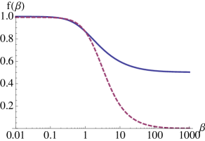
Figure 2: Low density results for the dimensionless friction coefficient increment as function of the dimensionless external force parameter $\beta=F_{\rm ex}a/(k_{B}T)$. Continuous line: exact result from Ref. Squires and Brady (2005). Dashed line: our MCT result.

Note that the approximation made to obtain the expression (98) was to completely neglect the memory integral, and the latter also contains the external force. Such an approximation might not be valid for large ${\bf F}_{ex}$. The large $\beta$-limit turns out to be singular in the low density theory Squires and Brady (2005) and this could also hold for our mode-coupling equations. This issue surely deserves a more thorough analysis including the numerical solution of the full time-dependent equation for the tracer density correlator.

The elementary consideration here is just aimed to show that even the simplest reasonable approximation (98) for the tracer correlator, in combination with the mode-coupling expression (85) for the force-force correlator, is already capable to explain the thinning effect. This is due to increasingly strong time oscillations of the integrand in eq. (93), which cut off larger and larger portions of the integrand with increasing $F_{ex}$.

III.2 Long time limit of the tracer density correlator

After considering the low-density dynamics in the last section, we turn now to the high-density “statics”. I.e. we will assume that we are above the critical point where the colloidal bath forms a glass ($\varphi>\varphi_{c}$). The first question then concerns the existence and force dependence of the long time limits

$$f^{s}_{\bf q} = \lim_{t\rightarrow\infty}\phi^{s}_{\bf q}(t)$$ (105)

$$f_{\bf q} = \lim_{t\rightarrow\infty}\phi_{\bf q}(t)$$ (106)

of the tracer and the bath density correlators. We restrict ourself here to the case of the equal size of the tracer and the bath particle so that $\alpha=1$ holds and only the bath volume fraction $\varphi$ remains as the control parameter. The existence of a finite probe ’non-ergodicity’ parameter signals that probe density fluctuations remain frozen-in, and that the probe can not explore the whole volume $V$. A $f^{s}_{\bf q}>0$ signals that the probe is localized.

For $t\rightarrow\infty$, the full time-dependent MCT equations (54), (80) reduce to the “static” (i. e. time-independent) equations

$$\frac{\omega_{\bf q}^{2}\,f^{s}_{\bf q}}{1-f^{s}_{\bf q}} = M^{s,\mbox{\tiny irr}}_{\bf q}(f^{s},\,f),$$ (107)

$$\frac{f_{\bf q}}{1-f_{\bf q}} = M^{\mbox{\tiny irr}}_{\bf q}(f),$$ (108)

(the derivation of the eq. (107) for the tracer straightforwardly follows the steps of the standard MCT Götze (2009)). Equations (107), (108) are much easier to treat than the full time-dependent equations because no memory integrals over many time decades have to be evaluated. Still, they contain a wave vector integration and hence represent a coupled system of equations for all ${\bf q}$.

In order to be solved numerically, the long time limit equations (107), (108) have to be rewritten as fixed point equations:

$$f_{\bf q} = \frac{M^{\mbox{\tiny irr}}_{\bf q}}{1+M^{\mbox{\tiny irr}}_{\bf q}},$$ (109)

$$f^{s}_{\bf q} = \frac{M^{s,\mbox{\tiny irr}}_{\bf q}}{\omega_{\bf q}^{2}+M^{s,\mbox{\tiny irr}}_{\bf q}}.$$ (110)

Starting with the initial values $f_{\bf q}=1$, $f^{s}_{\bf q}=1$ for all ${\bf q}$, the right-hand side of eqs. (110), (109) is evaluated and then used as input for the next iteration, until the desired precision is reached .

The spatial symmetry properties of the tracer and bath correlators dictate the choice of the discretization scheme for $f^{s}_{\bf q}$ and $f_{\bf q}$ in the $q$-space. Since the bath correlator is not affected by the external force, as was discussed in Section II.5.2, $f_{q}$ retains its spherical symmetry so that it can be taken as input for the equation (110) from the standard isotropic MCT calculation. An equidistant $q$-grid is chosen here with $100$ $q$-points for $qa\in(0,\,20)$ and the so-called “Bengtzelius trick” (see Bengtzelius et al. (1984) for details) allows to reduce the computational complexity during the calculation of the memory integral.

As for $f^{s}_{\bf q}$, the external force introduces a preferred direction in space and thus breaks the spherical symmetry. This means that in contrast to the isotropic calculation in the absence of ${\bf F}_{ex}$, one explicitly has to resolve the angular structure of $f^{s}_{\bf q}$. One symmetry still remains, namely the rotational symmetry around ${\bf F}_{ex}$. Thus, it is enough to specify the magnitude $q$ and the angle $\theta$ between the vectors ${\bf q}$ and ${\bf F}_{ex}$ in order to determine $f^{s}_{\bf q}$ uniquely.

We thus introduce spherical coordinates with the $z$-axis pointing in ${\bf F}_{\rm ex}$-direction and assume the wave vector ${\bf q}$ to lie in the $x$-$z$ plane. The property $f^{s}_{-\bf q}=f^{s\,*}_{\bf q}$ (which we assume to be valid, see discussion in Section II.6) allows us to confine the angle $\theta$ to the interval $(0,\frac{\pi}{2})$. Note however that despite this quasi-2d nature of the problem, the integration in the memory kernel includes all the wave vectors and cannot be reduced to a two-dimensional one. So, the polar angle $\phi$ also has to be included there, too.

Since the angles $\theta$ enter in eqs. (110) only via scalar products of vectors ${\bf q}$, ${\bf p}$ and ${\bf F}_{\rm ex}$ with each other (see relations (60), (79) for $\omega_{\bf q}$ and $M^{s,\mbox{\tiny irr}}_{\bf q}$), i. e. only as $\cos\theta$ or $\sin\theta$, it appears reasonable to change the variable from $\theta$ to $y=\cos\theta$ and employ the relation $\int_{0}^{\pi}d\theta\,\sin\theta\,f(\theta)=\int_{0}^{1}dy\,f(y)$ in calculating the wave vector integral entering $M^{s,\mbox{\tiny irr}}_{\bf q}$.

Since the $f_{\bf q}$-s enter the tracer equations (110) as input, the same equidistant $q$-grid is chosen for $f^{s}_{\bf q}$ as for $f_{\bf q}$. The $y$- and $\phi$-grids are also chosen equidistant with $30$ points for $y\in(0,1)$ and $20$ points for $\phi\in(0,2\pi)$.

Finally, as the equilibrium structural input, the Percus-Yevick structure factor Hansen and McDonald (1986); Percus and Yevick (1958) is used.

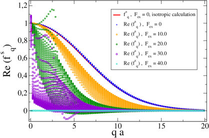
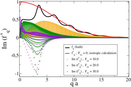
Figure 3: (Color online). Long time limit of the tracer density correlator (upper panel shows the real and lower panel the imaginary parts) as function of the wave vector magnitude $q$ for different angles $\theta$ (see text) and different $F_{ex}$. The bath volume fraction is $\varphi=0.52$. The two $f^{s}_{q}$ at $F_{\rm ex}=0$ in the upper panel show that the used angle-discretization is fine enough to recover the known isotropic result. In the lower panel the collective $f_{q}$ is included as reference. The rapid variations in all $f_{q}$ below $qa<0.5$ are discretization artifacts which do not affect the results for larger $q$.

The results of our numerical calculations for $f^{s}_{\bf q}$ are shown in Fig. 3. The value of the control parameter $\varphi$ was choose to be $0.52$, i. e. closely above the glass transition point $\phi_{c}\approx 0.516$ of quiescent MCT. The real and the imaginary parts of $f^{s}_{\bf q}$ are plotted as function of $q$ and the different curves for the same force value correspond to the different values of angle $\theta$. $F_{ex}$ is given in the dimensionless units of $k_{B}T/a$ (see eq. 104). The magnitude of the wave vector $q$ is given in units of $1/a$.

For $F_{ex}=0$, no angle dependence is observed and the standard isotropic MCT result is recovered. As $F_{ex}$ increases from $0$ and $30$, the splitting of $f^{s}_{\bf q}$-s with $\theta$ becomes more and more pronounced, revealing the spatial anisotropy, which increases with the external force.

For $F_{ex}>40$, $f^{s}_{\bf q}$ appears to drop to zero for all ${\bf q}$. This is an indication of the bifurcation transition in the equations (107): there is a certain critical force $F^{c}_{ex}$, above which only the (always existing, trivial) zero solution of (107) becomes stable, whereas below $F^{c}_{ex}$ the numerically found non-zero solution is stable.

Unfortunately, the numerics becomes unstable for $30<F_{\rm ex}<40$, so that we cannot approach the region of the critical force value arbitrarily closely. But the observed trends in the $F_{ex}$-dependence of the curves suggest that the transition is continuous (“of type A” in the MCT classification). I. e. for every ${\bf q}$, $f^{s}_{\bf q}$ goes down to zero continuously with increasing $F_{ex}$. At the bifurcation point, $f^{s}_{\bf q}$ becomes zero so that the two solution branches of eq. (107) coalesce.

The physical meaning of the bifurcation transition is that the cage surrounding the probe becomes weaker with increasing external force until the tracer gets “pulled free” out of the cage and depins from the glassy matrix. In Gazuz et al. (2009), we showed the results for the quantity $f^{s}({\bf r})$, which is the Fourier backtransform of $f^{s}_{\bf q}$ and has a very clear physical meaning; see eq. (43) and discussion after it. It can be related to the “shape” of the cage. The results for $f^{s}({\bf r})$, discussed in Gazuz et al. (2009), were obtained numerically from the $f^{s}_{\bf q}$, which seem not so easy to interpret, at first glance. It is still possible, however, to relate the observed features in the behaviour of $f^{s}({\bf r})$ (see Fig. 2 of Ref. Gazuz et al. (2009)) to the features of the $f^{s}_{\bf q}$-curves (Fig. 3).

First, we see that for $F_{\rm ex}=10$, the real parts of $f^{s}_{\bf q}(q)$ are monotonously decaying and the imaginary parts have one maximum for all values of $\theta$. Furthermore, the shape of the curves resembles the one obtained from the $\theta$-independent real function $f^{s}_{\bf q}(F_{\rm ex}=0)$ by multiplying by the prefactor $\exp(i\,{\bf q}\cdot\delta{\bf r})=\cos(q\,\delta r\cos\theta)+i\sin(q\,\delta r\cos\theta)$:

$$f^{s}_{\bf q}(F_{\rm ex})\approx f^{s}_{\bf q}(F_{\rm ex}=0)\,\exp(i\,{\bf q}\cdot\delta{\bf r}(F_{\rm ex})),$$ (111)

where we assume $\delta{\bf r}||{\bf F}_{\rm ex}$. Due to the translation theorem of the Fourier transform theory, this prefactor corresponds to the shifting of the $f^{s}({\bf r})(F_{\rm ex}=0)$-distribution by a vector $\delta{\bf r}\sim{\bf F}_{\rm ex}$. This is in accordance with our observations for the behaviour of $f^{s}({\bf r})$. For higher values of $F_{\rm ex}$, for some values of $\theta$ the real parts of the curves $f^{s}_{\bf q}(q)$ become non-monotonous, whereas the imaginary parts exhibit a maximum and a minimum. This complicated behaviour causes subtle features in the shape of the $f^{s}({\bf r})$-distribution discussed in Gazuz et al. (2009) (anisotropy with respect to the maximum, “dent”).

Finally, we discuss some peculiar features in the behaviour of the imaginary part of $f^{s}_{\bf q}$. For the direction perpendicular to ${\bf F}_{\rm ex}$, the imaginary part of $f^{s}_{\bf q}$ should vanish. This is the consequence of the relation $f^{s}_{\bf-q}=f^{s\,*}_{\bf q}$ and the rotational symmetry around ${\bf F}_{ex}$, which implies $f^{s\,*}_{{\bf q}^{\perp}}=f^{s}_{{\bf q}^{\perp}}$ for ${\bf q}^{\perp}\cdot{\bf F}_{\rm ex}=0$, so that

$$\Im\{f^{s}_{\bf q}\}=0\quad\quad\mbox{for}\quad{\bf q}\bot{\bf F}_{ex}$$ (112)

should apply.

For $F_{ex}=10$, we indeed observe this behaviour (which is also in agreement with our approximation (111)), whereas for higher force values, a strong dip is observed for $\Im\{f^{s}_{\bf q}\}(q)$ at $qa\approx 3$, for the $\theta$-values closest to $\pi/2$, whereas at $q=0$, $\Im\{f^{s}_{\bf q}\}(q)$ seems to diverge for all $\theta$. Since $\Im\{f^{s}_{\bf q}\}$ is antisymmetric in ${\bf q}$, this behaviour signalizes the discontinuity of the function $\Im\{f^{s}_{\bf q}\}({\bf q})$ at the plane ${\bf q}\bot{\bf F}_{\rm ex}$.

It is easy to see that the origin of this discontinuity lies in the presence of the term $\omega_{\bf q}^{2}$, which enters the long time limit eq. (110) under the denominator on the right hand side. The term $\omega_{\bf q}=D_{s}\,(q^{2}-i\,{\bf q}\cdot{\bf F}_{ex})$ itself obviously has the property $\Im\{\omega_{\bf q}\}=0$ for ${\bf q}\bot{\bf F}_{ex}$, so the same should be valid for its inverse. The inverse however, is divergent at the point ${\bf q}=0$, so that $\Im\{1/\omega_{\bf q}\}=0$ applies everywhere on the plane ${\bf q}\bot{\bf F}_{ex}$ except for the singular point ${\bf q}=0$.

The discussed behaviour of the term $1/\omega_{\bf q}$ is relevant for $f^{s}_{\bf q}$, since if one approaches the bifurcation transition, the function $f^{s}_{\bf q}({\bf q})$ becomes confined to a narrow region around the origin in the ${\bf q}$-space and the same applies also for the memory function $M^{s,\mbox{\tiny irr}}_{\bf q}$. So, as a very rough first guess, $M^{s,\mbox{\tiny irr}}_{\bf q}$ can be neglected in the denominator of eq. (110), as a “small” quantity. As a next approximation, one can use an ${\bf q}$-independent ansatz for $M^{s,\mbox{\tiny irr}}_{\bf q}$ in (110). In this way it is already possible to obtain the structure of the ${\bf q}$-dependence very similar to that observed for $f^{s}_{\bf q}$ in our numerical solution of eq. (110) at high force values.

We believe that the qualitative discussion of the properties of $f^{s}_{\bf q}$ given here, already contributes to a deeper understanding of our numerical results. The origin of the unphysical results for $f^{s}_{\bf q}$ at larger forces remains to be clarified. It should be possible to extract also quantitative results for the limiting cases $F_{\rm ex}\rightarrow 0$ and $F_{\rm ex}\rightarrow F_{\rm ex}^{c}$ by either performing expansions in $F_{\rm ex}$ (for $F_{\rm ex}\rightarrow 0$) in eq. (110) or an appropriate asymptotic expansion assuming the smallness of $f^{s}_{\bf q}$ (for $F_{\rm ex}\rightarrow F_{\rm ex}^{c}$). This will be a subject of future work. For the case of schematic models, the latter has recently been achieved Gnann and Voigtmann (2012).

IV Schematic Models

The bifurcation scenario we deduced from the wavevector dependent equations of motion is continuous. At the critical force $F_{\rm ex}^{c}$, the long time limit $f^{s}_{\bf q}$ vanishes, as has been found in type A transitions within quiescent MCT Götze (2009). The universal properties close to quiescent type A transitions could be analyzed in schematic models, because all wavevectors are coupled strongly at the bifurcation. Here we show that the simplest schematic models containing complex correlators, which can be derived from the full theory under external force, again describe a continuous delocalization transition at a critical force. They can thus be used to gain insight into the more universal phenomena close to the bifurcation.

IV.1 Construction of the models

Simplified schematic models for tracer density fluctuations can be constructed by considering only two wave vectors ${\bf k},-{\bf k}$ with ${\bf k}\,||\,{\bf F}_{ex}$ and neglecting the contribution of all the other wave vectors to the memory function. Due to the property $\phi^{s}_{-\bf k}=\phi^{s\,*}_{\bf k}$, the system of equations for $\phi^{s}_{\bf k}$, $\phi^{s}_{-\bf k}$, obtained in this way, reduces to the following single equation for $\phi^{s}_{\bf k}$:

$$\partial_{t}\,\phi^{s}_{\bf k}(t)=-D_{s}(k^{2}-ikF_{ex})\,\phi^{s}_{\bf k}(t)\quad\quad\quad\quad\quad\quad\quad\quad$$ (113)

$$-\int_{0}^{t}dt^{\prime}\,v_{\bf k}k^{2}\,\phi^{s}_{\bf k}(t-t^{\prime})^{*}\,\phi_{2{\bf k}}(t-t^{\prime})\,\partial_{t^{\prime}}\phi^{s}_{\bf k}(t^{\prime})\,,$$

where $v_{\bf k}=4{S_{k}^{s}}^{\,2}/NS_{2k}$. We see that the force dependence of the memory function drops in eq. (113). Further simplification can be achieved if we introduce a scale for lengths so that $k=1$, rescale time so that $D_{s}=1$ and model the behaviour of the bath correlator $\phi_{k=1}\equiv\phi$ with the standard F12-model Götze (1991). For simplicity we set its short time coefficient equal to the tracer’s.

We finally arrive at

$$\!\!\!\!\!\!\!\!\partial_{t}\,\phi^{s}(t) = -\omega\,\phi^{s}(t)-\int_{0}^{t}dt^{\prime}\,m^{s}(t-t^{\prime})\,\partial_{t^{\prime}}\phi^{s}(t^{\prime}),$$ (114)

$$\!\!\!\!\!\!\!\!\partial_{t}\,\phi(t) = -\phi(t)-\int_{0}^{t}dt^{\prime}\,m(t-t^{\prime})\,\partial_{t^{\prime}}\phi(t^{\prime}),$$ (115)

with the complex frequency

$$\omega=1-i\,F_{ex}$$ (116)

and the memory functions

$$m^{s}(t) = v_{s}\,\phi^{s*}(t)\phi(t)$$ (117)

$$m(t) = v_{1}\,\phi(t)+v_{2}\,\phi^{2}(t).$$ (118)

This schematic model will be called the $F_{ex}$-Sjögren model. It extends the original Sjögren model (proposed in Ref. Sjögren (1986)) for the tagged particle dynamics in a host fluid for the case of external driving with the force $F_{\rm ex}$. From the described rescalings, it is obvious that in the schematic model $F_{\rm ex}$ is measured in thermal energy divided by the length used to rescale the wavevector in Eq. (113).

A modification of the model (114) is of interest, namely the one where $\phi(t)\equiv 1$ is set:

$$\partial_{t}\,\phi^{s}(t)=-\omega\,\phi^{s}(t)-\int_{0}^{t}dt^{\prime}\,v_{s}\,\phi^{s*}(t-t^{\prime})\,\partial_{t^{\prime}}\phi^{s}(t^{\prime})\ .$$ (119)

We call this model the $F_{ex}$-F1 model. It extends the well-known $F1$-model Götze (1991) (corresponding to the case $F_{ex}=0$) which was introduced in connection with the mode-coupling theory for the Lorentz model. The latter describes a tagged particle in an array of immobile randomly distributed scatterers. As we shall see in Sec. IV.7.1, the $z=0$ value for the Laplace transform of our $F_{ex}$-F1 model is available in exact form.

IV.2 The phase diagrams

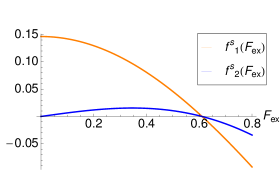
Figure 4: Real and imaginary parts of the long time limit of the tracer density correlator as functions of the external force ($v_{2}=2.0$, $v_{s}=4.0$).

In this section we consider the long time limit $f^{s}=f^{s}_{1}+if^{s}_{2}$ of the correlator $\phi^{s}(t)$. For our schematic models, the condition (107) reduces to

$$\frac{\omega\,f^{s}}{1-f^{s}}=m^{s}(f^{s},f),$$ (120)

Considering the real and imaginary of eq. (120) separately, we obtain the system of equations

$$F_{1}(f^{s}_{1},\,f^{s}_{2})=0$$ (121)

$$F_{2}(f^{s}_{1},\,f^{s}_{2})=0$$ (122)

for $f^{s}_{1}$, $f^{s}_{2}$, where

$$F_{1} = f^{s}_{1}+F_{ex}f^{s}_{2}-v_{s}f\,(f^{s}_{1}-{f^{s}_{1}}^{2}-{f^{s}_{2}}^{2})$$ (123)

$$F_{2} = f^{s}_{2}-F_{ex}f^{s}_{1}+v_{s}ff^{s}_{2}.$$ (124)

Eq. (122) yields the linear relationship

$$f^{s}_{2}=\alpha\,f^{s}_{1}$$ (125)

between $f^{s}_{2}$ and $f^{s}_{1}$ with

$$\alpha=\frac{F_{ex}}{1+v_{s}\,f}\,,$$ (126)

which can be inserted into eq. (121) to obtain a quadratic equation for $f^{s}_{1}$. Its first trivial solution is $f^{s}_{1}=0$. The second solution is:

$$f^{s}_{1}=\frac{-\alpha\,F_{ex}+v_{s}\,f-1}{v_{s}\,f\,(1+\alpha^{2})}\;.$$ (127)

In the absence of the external force we have $\alpha=0$, so $f^{s}_{2}=0$. I. e. the tracer correlator is real and the result of the original Sjögren model is recovered:

$$f^{s}_{1}=1-\frac{1}{v_{s}\,f}\,.$$ (128)

There is a bifurcation at $v_{s}^{c}=1/f$: for $v_{s}<v_{s}^{c}$, the long time limit of $\phi_{s}(t)$ is zero (since it cannot be negative) and for $v_{s}>v_{s}^{c}$ it has a non-zero value which is given by eq. (128). This consideration is valid for $f>0$, i. e., if the bath is in a glassy state. If $f=0$, then $f^{s}_{1}=0$ always holds.

Now, let us assume that for $F_{ex}=0$, the tracer is in an arrested state: $f^{s}_{1}>0$. Can this state be “molten” by the external force field ? We look at the behaviour of $f^{s}_{1}$ as a function of the external force for fixed values of $f$ and $v_{s}$. Eqs. (126),(127) yield:

$$f^{s}_{1}=\frac{(1+v_{s}\,f)((v_{s}\,f)^{2}-1-F_{ex}^{2})}{v_{s}\,f\,((1+v_{s}\,f)^{2}+F_{ex}^{2})}$$ (129)

In Fig. 4, $f^{s}_{1}$ and $f^{s}_{2}$ are plotted as function of $F_{\rm ex}$ for fixed parameter values $v_{2}=2.0$, $v_{s}=4$, . We see that our schematic model exhibits the critical force at which the tracer becomes delocalized, i. e. where the depinning transition occurs.

Figure 5: Phase diagram sketches of the schematic model for fixed $f>f^{c}$ (upper panel) and fixed $v_{s}$ (lower panel).

From eq. (129), we obtain

$$F^{c}_{ex}=\sqrt{(v_{s}\,f)^{2}-1}$$ (130)

for the critical force $F^{c}_{ex}$, at which real and imaginary part of $f^{s}$ become zero together. Eq. (130) can be visualized in form of phase diagrams, (schematically) shown in Fig. 5. Note that in the fixed $v_{s}$ diagram the horizontal axis corresponds to the variable $\varepsilon(f)$, which measures the distance from the glass transition point of the bath (see Sec. IV.4 for the definition) so that $\varepsilon=0$ corresponds to $f=f^{c}$.

The analytical results for the long time limit derived above for the $F_{ex}$-Sjögren model obviously apply for the $F_{ex}$-F1 model if one sets $f=1$ in the corresponding expressions.

IV.3 Bifurcation analysis

The purely algebraic consideration in the last Section can be completed by the analysis of the bifurcation scenario for the eq. (120).

At the critical force, the two solutions $f^{s}=0$ and the one given by eqs. (127), (125) coalesce. In order to clarify the geometry of the problem, we look at the solution space of eq. (120), namely the ($f^{s}_{1}$, $f^{s}_{2}$)-plane. Since the complex conjugation is involved, being a nonanalytic operation, no use can be made of the complex analysis .

So, instead of the complex eq. (120) we have to analyze the equivalent system of real equations (121), (122). Each of them defines a curve in the solution plane. The curves are of the order not higher then quadratic. Generically, they intersect in two points. The bifurcation occurs, when the two curves are just tangent to each other, so that there is only one intersection point identical with the osculation point.

The normals to the curves defined by eqs. (121) and (122) are given by the gradient vectors $(\partial F_{1}/\partial f^{s}_{1},\,\partial F_{1}/\partial f^{s}_{2})$ and $(\partial F_{2}/\partial f^{s}_{1},\,\partial F_{2}/\partial f^{s}_{2})$, respectively. They have to be parallel at the bifurcation point (since the curves have to be tangent, as discussed above) and this is equivalent to the requirement

$$\det J=0$$ (131)

for the matrix $J$ with the elements $J_{ik}=\partial F_{i}/\partial f^{s}_{k}$, where $i,k\in\{1,2\}$. From eqs. (123), (124) we obtain:

$$J=1\!\!\mbox{I}-I$$ (132)

with

$$I=\left(\begin{array}[]{cc}v_{s}f&-F_{ex}\\ F_{ex}&-v_{s}f\end{array}\right),$$ (133)

and the unity matrix $1\!\!\mbox{I}$. So, condition (131) is equivalent to the condition $\det I=1$, which immediately yields the expression (130) for the critical force.

Besides from recovering the result for the critical force from the last section, the considerations here enable us to learn more about the bifurcation. Let us look at the eigenvalues $\lambda$ of the matrix $I$. They are solutions of the characteristic equation $\det(I-\lambda\,1\!\!\mbox{I})=0$, which yields

$$\lambda^{2}=v_{s}^{2}f^{2}-F_{ex}^{2}.$$ (134)

The eigenvalue $\lambda=1$ corresponds exactly to $F_{ex}=F^{c}_{ex}$. This eigenvalue is not degenerated. This means, the bifurcation is of the codimension one Arnol’d (1992).

IV.4 Effect of the external force on the correlators

We want to consider now the full time dependence of the correlators and look, how it is influenced by the external force. The equations (114), (119) are solved numerically using the algorithm described in Fuchs et al. (1991) applied to real and imaginary part individually. The results are summarized in Fig. 6 for typical values of the parameters.

The behaviour of the schematic models of the standard MCT well known from Refs. Sjögren (1986); Götze (1991, 2009) will be taken as reference where appropriate in the following. For the parameters of the F12 model the relation holds

$$v^{c}_{1}=v^{c}_{2}\,(\frac{2}{\sqrt{v^{c}_{2}}}-1),$$ (135)

for $v^{c}_{1}$, $v^{c}_{1}$ lying on the bifurcation line, separating the liquid phase from the glass phase. We introduce also the parameter $\varepsilon$ which measures the distance from the glass transition line and is related to $v_{2}=v^{c}_{2}+\delta v_{2}$ and $v_{1}=v^{c}_{1}+\delta v_{1}$ by

$$\varepsilon=\frac{\delta v_{1}\,f^{c}+\delta v_{2}\,{f^{c}}^{2}}{1-f^{c}}$$ (136)

with $f^{c}=1-\frac{1}{\sqrt{v^{c}_{2}}}$. In the following, the parameters will be chosen such that $v_{2}=v^{c}_{2}$, so that $\delta v_{2}=0$. Thus, specifying the values of $v_{2}$ and $\varepsilon$ completely determines the parameters of the F12-model according to the eqs. (136), (135).

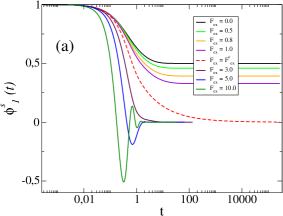
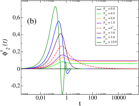
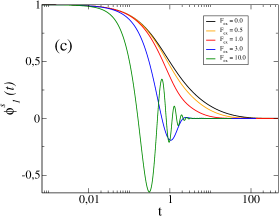
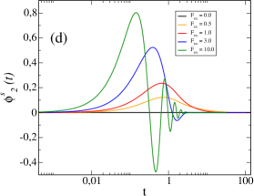
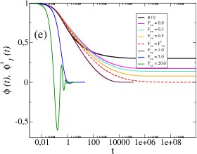
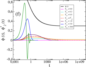
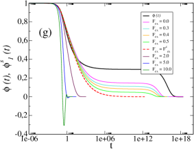
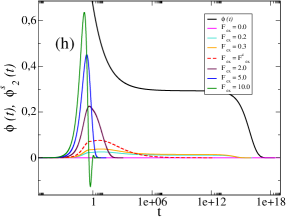
Figure 6: (Color online). Time-dependence of the probe-particle correlators from the schematic models with increasing $F_{ex}$. The left column shows the real parts, the right column the imaginary parts. Panels (a-f) correspond to glass states, where the bath is nonergodic; panels (g,h) are for a fluid state, here $F_{\rm ex}^{c}=F_{\rm ex}^{c}(\epsilon=0)$. Panels (a-d) are for the $F_{\rm ex}$-F1 model where the bath is completely arrested ($\phi=1$), and panels (e-h) are for the $F_{ex}$-Sjögren model. Panels (c,d) are for a weakly coupled probe ($v_{s}<v_{s}^{c}$), which remains mobile in glass even at vanishing force. The parameter values are $v_{s}=2.0$ (a,b), $v_{s}=0.8$ (c, d) and $\varepsilon=10^{-4}$, $v_{2}=2.0$, $v_{s}=4.0$ (e, f), $\varepsilon=-10^{-7}$, $v_{2}=2.0$, $v_{s}=4.0$ (g, h).

First we consider the case, where the tracer is in the arrested state for $F_{\rm ex}=0$. For the $F_{\rm ex}$-F1 model this means $v_{s}>1$, and for the $F_{ex}$-Sjögren model $\varepsilon>0$ and $v_{s}>1/f$. The corresponding plots are shown on panels (a,b) (for the $F_{ex}$-F1 model) and (e,f) (for the $F_{ex}$-Sjögren model) of Fig. 6. We can see that the behaviour of the long time limit of the tracer correlator is in accordance with the results of Sect. IV.2 (see Fig. 4). For the real part, the long time limit goes down to zero monotonously with increasing $F_{\rm ex}$, whereas for the imaginary part, the long time limit first increases from the zero value at $F_{\rm ex}=0$ and then goes down to zero, until the critical force value $F_{\rm ex}^{c}$ is reached (see the dashed thick red line in the plots). For $F_{\rm ex}>F_{\rm ex}^{c}$, the long time limit remains zero.

For $F_{\rm ex}<F_{\rm ex}^{c}$, the real part of the correlator is a monotonously decaying function of time, whereas the imaginary part exhibits a maximum. For $F_{\rm ex}>F_{\rm ex}^{c}$, both the real and the imaginary parts of the tracer correlator decay faster and faster with increasing $F_{\rm ex}$ and eventually start to oscillate. These oscillations are due to the $F_{\rm ex}$-dependent term $\omega$ (see eqs. (114), (116), (119)), which dominates at high forces. The oscillations thus arise for all bath states at larger forces (see Fig. 6, panels (a-h)).

For the case that the bath is in the arrested state but the coupling between the tracer and the bath is small (see panels (c-d) of Fig. 6), the long time limit of the tracer correlator is equal to zero for all values of $F_{\rm ex}$. The behaviour of $\phi^{s}(t)$ is similar to that for the case of strong probe-bath coupling for $F_{\rm ex}>F_{\rm ex}^{c}$.

Finally, for the case of the liquid bath (panels (g-h) of Fig. 6), we can see that besides lowering the value of the intermediate $\beta$-plateau with increasing $F_{\rm ex}$ (this effect corresponds to the effect of decreasing long time limit with increasing $F_{\rm ex}$ for $\varepsilon>0$), also the time scale of the $\alpha$-process (i. e. the final decay from the $\beta$-plateau to zero) decreases. After the critical value $F^{c}_{ex}(\varepsilon=0)$ is reached, the $\beta$-plateau becomes zero and the difference between the $\beta$-process and the $\alpha$-process disappears. The behaviour for $F_{ex}>F^{c}_{ex}(\varepsilon=0)$ is similar to that of the case $\varepsilon>0$ (as was already mentioned in this section): the overall time scale of the decay decreases and for large enough $F_{\rm ex}$, the tracer correlator starts to oscillate.

In the next sections, we consider the $\beta$-relaxation and the $\alpha$-relaxation regions of the $F_{ex}$-Sjögren model in more detail and make some quantitative predictions.

IV.5 The $\beta$-correlators

In this section we consider the behaviour of the correlators around the $\beta$-relaxation plateau and perform a (non-linear) stability analysis of the arrested/localized part of the correlator. Here, classical MCT has provided the deepest insights by deriving results like the factorization theorem and power-law relaxation during the so-called $\beta$-process. The $q$-dependent factorization theorem shows that the dynamics on all length scales follows a single, time-dependent function, the so-called $\beta$-correlator $G(t)$. It depends sensitively on the separation to the MCT bifurcation and introduces algebraic decay into the dynamics. We perform the non-linear stability analysis in order to investigate the de-localization transition at finite force in more detail.

IV.5.1 The $\beta$-scaling equation

We use the ansatz

$$\phi^{s}(t) = f^{s}+G^{s}(t),$$ (137)

$$\phi(t) = f+G(t)$$ (138)

with the assumptions that $f^{s},\,f$ fulfill the long-time limit equation (120) and the $\beta$-correlators $G^{s}(t)$, $G(t)$ are small

$$|G^{s}(t)|,\,|G(t)|\ll 1.$$ (139)

Using the standard steps (partial integration etc.), we rewrite eq. (114) in the form

$$\partial_{t}\phi^{s}(t)=-\omega\,\phi^{s}(t)+m(t)-\frac{d}{dt}\int_{0}^{t}dt^{\prime}\,m(t-t^{\prime})\,\phi^{s}(t^{\prime})\,.$$ (140)

We insert eqs. (137), (138) into (140) and obtain

$$\partial_{t}G^{s}(t)=-\omega\,(f^{s}+G^{s}(t))+v_{s}\,({f^{s}}^{*}+{G^{s}}^{*}(t))\,(f+G(t))-\frac{d}{dt}\,\int_{0}^{t}dt^{\prime}\,v_{s}\,({f^{s}}^{*}+{G^{s}}^{*}(t-t^{\prime}))\,(f+G(t-t^{\prime}))\,(f^{s}+G^{s}(t^{\prime}))$$ (141)

While eq. (141) has not been solved yet for all relevant cases, a number of solutions exist and provide insight into the tracer dynamics close to delocalization.

If we retain only the terms of the order not higher than linear in $G^{s}$, $G$ in eq. (141), neglect the time derivative and make use of eq. (120), we obtain

$$G^{s}(t)\,\left({f^{s}}^{*}f-\frac{\omega}{v_{s}}\right)+{G^{s}}^{*}(t)\,f\,(1-f^{s})\quad\quad\quad$$

$$+\,G(t)\,({f^{s}}^{*}-|f^{s}|^{2})=0\quad\quad$$ (142)

IV.5.2 Factorization theorem for fluid states in the $F_{ex}$-Sjögren model

Here we want to consider the $F_{ex}$-Sjögren model in the liquid state ($\varepsilon<0$) for the case that the external force is smaller than its critical value for $\varepsilon=0$. This means that the $\beta$-relaxation plateau is non-zero.

We consider eq. (142) and choose $f^{s}$ to be the long time limit of the tracer correlator for $\varepsilon=0$. So, $f^{s}\neq 0$ and eq. (142) can be considered as a linear equation for $G^{s}(t)$ with the given $G(t)$. Expressing $\omega/v_{s}$ in terms of the known functions of $F_{ex}$, namely $f^{s}_{1}$ and $f^{s}_{2}$ and using the long-time limit equation (120), we obtain

$$-G^{s}(t)\,{f^{s}}^{*}\,f+{G^{s}}(t)^{*}\,f^{s}\,f\,(1-f^{s})+G(t)\,|f^{s}|^{2}\,(1-f^{s})=0$$ (143)

In terms of $G^{s}_{1}(t)$, $G^{s}_{2}(t)$, i. e. the real and imaginary parts of $G^{s}(t)$, eq. (143) can be easily solved with the result

$$G^{s}_{1}(t) = h_{1}\,G(t),$$ (144)

$$G^{s}_{2}(t) = h_{2}\,G(t),$$ (145)

where

$$h_{1} = \frac{|f^{s}|^{2}\,(2f^{s}_{1}\,{f^{s}_{2}}^{2}+(2f^{s}_{1}+{f^{s}_{2}}^{2}-{f^{s}_{1}}^{2})\,(1-f^{s}_{1}))}{f\,(4{f^{s}_{2}}^{2}f^{s}_{1}\,(1-f^{s}_{1})-(2f^{s}_{1}+{f^{s}_{2}}^{2}-{f^{s}_{1}}^{2})\,({f^{s}_{2}}^{2}-{f^{s}_{1}}^{2}))}\quad$$ (146)

$$h_{2} = \frac{h_{1}\,f\,({f^{s}_{2}}^{2}-{f^{s}_{1}}^{2})+|f^{s}|^{2}\,(1-f^{s}_{1})}{2\,f\,f^{s}_{1}\,f^{s}_{2}}$$ (147)

This result generalizes the factorization theorem of MCT to forced probes. As a check, we set $F_{ex}=0$ and obtain the well-known result of the Sjögren model Götze (1991); Sjögren (1986):

$$G^{s}=G^{s}_{1}+iG^{s}_{2}=G^{s}_{1}=G\,\frac{1}{v_{s}f^{2}}.$$ (148)

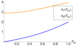
Figure 7: The critical amplitudes (eqs. (146), (147)) of the $F_{ex}$-Sjögren model in the fluid state ($v_{2}=2.0$, $v_{s}=4.0$, $F_{\rm ex}^{c}(\varepsilon=0)=0.61$).

The critical amplitudes $h_{1}$, $h_{2}$ are plotted in Fig. 7 as functions of $F_{ex}$ for fixed values of $v_{2}$ and $v_{s}$. Both functions increase monotonically in the (meaningful) region of the force values $F_{ex}<F^{c}_{ex}$. At $F_{ex}=0$, the function $h_{2}(F_{ex})$ starts linearly from zero, whereas $h_{1}(F_{\rm ex})$ starts quadratically at a non-zero value, as required by symmetry.

To check our results numerically, we plot the $\beta$-correlators (defined in Eqs. (137, 138)), first unscaled and then scaled according to the expressions (144), (145) in Fig. 8. We see, that $G^{s}_{1}(t)$, $G^{s}_{2}(t)$ indeed collapse on the master curve given by $G(t)$, if one is not too far away from the plateau. This holds for more than ten decades in time in Fig. 8.

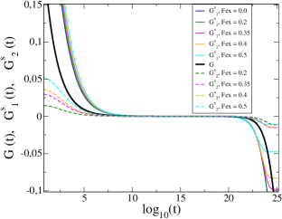
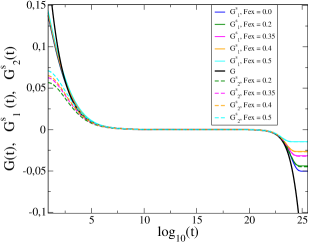
Figure 8: (Color online). Beta correlators, unscaled (upper panel) and scaled (lower panel) of the $F_{ex}$-Sjögren model in the fluid state for $F_{\rm ex}<F_{\rm ex}^{c}(\varepsilon=0)$ ($v_{2}=2.0$, $v_{s}=4.0$, $\varepsilon=-10^{-11}$, $F_{\rm ex}^{c}(\varepsilon=0)=0.61$).

IV.5.3 The critical correlators

In this section we want to consider the $\beta$-correlators at the critical force value $F_{ex}=F^{c}_{ex}$. So, we set $f^{s}=0$ in eq. (142) and obtain

$$G^{s}(t)\,\omega+{G^{s}}^{*}(t)\,v_{s}f=0.$$ (149)

As can be readily seen, in terms of $G^{s}_{1}(t)$, $G^{s}_{2}(t)$ the above equation can be rewritten as

$$J\,\left(\begin{array}[]{c}G^{s}_{1}(t)\\ G^{s}_{2}(t)\end{array}\right)=0,$$ (152)

where the matrix $J$ is identical with the one given by eqs. (132), (133). Thus, except from the trivial solution $G^{s}_{1}(t)=G^{s}_{2}(t)=0$, the solution of eq. (149) exists only when the determinant of the matrix $J$ vanishes, which is exactly the bifurcation condition, as discussed in Sect. IV.3. If it is fulfilled, the solution of eq. (149) is not unique and represents a relationship between $G^{s}_{1}(t)$ and $G^{s}_{2}(t)$.

In our case the codimension of the bifurcation, i. e. the dimension of the critical space is one, as was shown in Sec. IV.3. Thus at the bifurcation, the correlators $G^{s}_{1}(t)$, $G^{s}_{2}(t)$ are proportional to the critical eigenvector of the stability matrix and thus to each other.

Considering also the next-to-leading (quadratic) terms in eq. (141) and still assuming $f^{s}=0$, we obtain

$$-G^{s}(t)\,\frac{\omega}{v_{s}}+{G^{s}}^{*}(t)\,(f+G(t))=\frac{d}{dt}\int_{0}^{t}dt^{\prime}\,G^{s}(t^{\prime}){G^{s}}^{*}(t-t^{\prime}).$$ (153)

For the $F_{ex}$-$F1$ model, we have to set $f=1$ and $G=0$ in eq. (153). The left-hand side of eq.(153) vanishes due to the condition (149) and we obtain the following equation for the critical $\beta$-correlator:

$$0=\frac{d}{dt}\int_{0}^{t}dt^{\prime}\,G^{s}(t^{\prime}){G^{s}}^{*}(t-t^{\prime}).$$ (154)

This equation can be solved by means of the power-law ansatz

$$G^{s}(t)=t^{x}+i\,t^{y}.$$ (155)

We get under the integral in eq. (154) the expression

$$t^{\prime x}\,(t-t^{\prime})^{x}+t^{\prime y}\,(t-t^{\prime})^{y}+i\,\left[t^{\prime y}\,(t-t^{\prime})^{x}-t^{\prime x}\,(t-t^{\prime})^{y}\right].$$ (156)

Using the identity

$$\frac{d}{dt}\int_{0}^{t}dt^{\prime}\,(t-t^{\prime})^{x}\,t^{\prime y}=t^{x+y}\frac{\Gamma(x+1)\Gamma(y+1)}{\Gamma(x+y+1)},$$ (157)

where $\Gamma(x)$ is the gamma function, we see that the imaginary part of the right-hand side in eq. (154) vanishes. The choice $x=y=-1/2$ lets also the real part of the right-hand side in eq. (154) vanish, since then the denominator in eq. (157) diverges.

We thus found the power law solution

$$G^{s}(t)=t^{-1/2}+i\,t^{-1/2}$$ (158)

of the equation (154), which gives the critical $\beta$-correlator of the $F_{\rm ex}$-F1 model. Fig. 9 shows the critical correlators for different values of the parameter $v_{s}$. We see that the power law (158) indeed holds both for the real (continuous lines) and the imaginary parts (dashed lines) asymptotically for large times. The solution (158) can still be multiplied by an arbitrary prefactor. This expresses the scale invariance of the eq. (154). The correct prefactor can be found by matching to the initial decay.

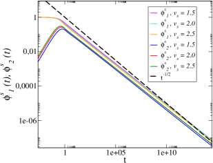
Figure 9: (Color online). The critical correlators of the $F_{ex}$-$F1$ model for different values of $v_{s}$. The thick black curve represents the asymptotic power law (158).

If we consider now the $F_{ex}$-Sjögren model, we get from eqs. (153), (149)

$${G^{s}}^{*}(t)\,G(t)=\frac{d}{dt}\int_{0}^{t}dt^{\prime}\,G^{s}(t^{\prime}){G^{s}}^{*}(t-t^{\prime}).$$ (159)

This equation has no simple power-law solution, since with the power-law ansatz, the imaginary part of its right-hand side would vanish, whereas the left-hand side would still have a non-vanishing imaginary part.

IV.6 The $\alpha$-relaxation

We want to consider now the $\alpha$-decay region of the $F_{\rm ex}$-Sjögren model for $\varepsilon<0$ (see panels (g-h) of Fig. 6 and the discussion at the end of Sec. IV.4) in more detail.

The $\alpha$-relaxation behaviour of the schematic model without the external force is a well known example of the second scaling-region of MCT, describing the final decay of the correlator on time scale $\tau$, the so-called final, or $\alpha$-relaxation time. For the present discussion we recall, that the second relaxation step of the correlators asymptotically (for $\varepsilon\rightarrow 0^{-}$) follows a scaling-function Götze (2009)

$$\phi(t)\simeq\tilde{\phi}\left(\frac{t}{\tau(\varepsilon)}\right).$$ (160)

As we saw in Sec. IV.4, the presence of the external force influences both the time scale of the $\alpha$-decay and the height of the $\beta$-plateau. So, a simple scaling law like (160) cannot work any more. However, if we rescale the amplitude of the correlator $\phi^{s}_{i}$ by the factor $\frac{f^{s}_{1}(F_{ex}=0)}{f^{s}_{i}(F_{ex})}$ ($i=1,\,2$), so that both $\phi^{s}_{1}$ and $\phi^{s}_{2}$ decay from the same ($F_{ex}=0$ real part-) plateau (see Fig. 10), we see that with increasing $F_{\rm ex}$, the shape of both $\phi^{s}_{1}$- and $\phi^{s}_{2}$-curves varies slightly. There is also some difference between the shape of $\phi^{s}_{1}$ and $\phi^{s}_{2}$ at the same value of $F_{\rm ex}$, which decreases with increasing $F_{ex}$ so that for $F_{ex}=1.4$ (slightly below the critical force) $\phi^{s}_{1}$ and $\phi^{s}_{2}$ almost match.

This observation justifies us to propose the (approximate) generalized ansatz

$$\phi^{s}(t)\simeq f^{s}(F_{\rm ex})\,\tilde{\phi^{s}}\left(\frac{t}{\tau^{s}(F_{ex},\varepsilon)}\right),$$ (161)

suggesting that there is still a universal decay function but accounting for the change in the plateau value. $\tilde{\phi^{s}}(t)$ is suggested to be real, which means that both the real and the imaginary parts of $\phi^{s}$ have the same shape. The precision of (161) can be considered as acceptable if one realizes that the change of the decay time scale with increasing $F_{\rm ex}$ by several orders of magnitude has a much stronger effect than the minor change in the shape of the curves.

To determine the tracer $\alpha$-time scale $\tau^{s}$, we match (161) to the $\beta$-decay law (see Sec. IV.5.2):

$$\phi^{s}_{i}(t)=f^{s}_{i}+h_{i}\,G(t)=f^{s}_{i}\,\left(1-\frac{h_{i}}{f^{s}_{i}}\,\left(\frac{t}{\tau(\varepsilon)}\right)^{b}\right)=\quad$$

$$=f^{s}_{i}\,\left(1-\left(\frac{t}{\tau(\varepsilon)}\,(f^{s}_{i}/h_{i})^{1/b}\right)^{b}\right),\quad$$ (162)

where the asymptotic form of the bath beta-correlator $G(t)=-\left(t/\tau(\varepsilon)\right)^{b}$ was used Götze (1991), to obtain

$$\tau^{s}_{i}(\varepsilon,\,F_{ex})=\tau(\varepsilon)\,\left(\frac{f^{s}_{i}}{h_{i}}(F_{ex})\right)^{1/b},$$ (163)

where $i=1,\,2$ corresponds to the real and imaginary part, respectively. This result will be used in the next section to analyse the low-force behavior of the tracer friction coefficient in a fluid host.

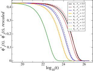
Figure 10: $\alpha$-decay of the correlators, rescaled in the amplitude according to their $\beta$-plateau values. The parameters are $v_{s}=6.0$ , $v_{2}=2.0$, $\varepsilon=-10^{-11}$ (this corresponds to $F^{c}_{ex}=1.445$).

IV.7 The tracer friction coefficient

Within the framework of the schematic models, where no wave vector dependence of the correlators is present, we define the friction coefficient increment following our considerations in Sec. II.3 as the time integral over the product of the real part of the tracer correlator and the bath correlator:

$$\Delta\zeta_{s}=\int_{0}^{\infty}dt\,\phi^{s}_{1}(t)\,\phi(t)$$ (164)

IV.7.1 $F_{ex}$-F1model

We start by considering first the $F_{ex}$-F1 model, since exact analytical results are available here. Eq. (119) reads in the Laplace space:

$$-i\,(z\,\widehat{\phi^{s}}(z)+1)=-(1-i\,F_{ex})\,\widehat{\phi^{s}}(z)-v_{s}\,(z\,\widehat{\phi^{s}}(z)+1)\,\widehat{\phi^{s}}^{*}(-z).$$ (165)

We use the following definition of the Laplace transform

$$\hat{f}(z)=LT[f(t)](z)\equiv i\,\int_{0}^{\infty}dt\,e^{izt}\,f(t),$$ (166)

with the properties

$$LT\left[\partial_{t}f(t)\right]\,(z) = -i\,(z\,\hat{f}(z)+f(0)),\quad\quad\quad$$ (167)

$$LT\left[\int_{0}^{t}ds\,f(s)\,g(t-s)\right]\,(z) = -i\,\hat{f}(z)\,\hat{g}(z),$$ (168)

$$LT\left[f^{*}(t)\right]\,(z) = -(\hat{f})^{*}(-z).$$ (169)

For the calculation of the friction coefficient, only the imaginary part of $\widehat{\phi^{s}}(z=0)$ is of interest, since $\widehat{\phi^{s}}(z=0)=-\int_{0}^{\infty}dt\,\phi^{s}_{2}(t)+i\,\int_{0}^{\infty}dt\,\phi^{s}_{1}(t)$. So, we have $\Delta\zeta_{s}=\Im\{\widehat{\phi^{s}}(z=0)\}$. We set $z=0$ in eq. (165), then the product $z\,\widehat{\phi^{s}}$ vanishes and for

$$\widehat{\phi^{s}}_{1} \equiv \Re\{\widehat{\phi^{s}}(z=0)\},$$ (170)

$$\widehat{\phi^{s}}_{2} \equiv \Im\{\widehat{\phi^{s}}(z=0)\}$$ (171)

we obtain the following system of equations

$$\widehat{\phi^{s}}_{1}+F_{ex}\,\widehat{\phi^{s}}_{2} = -v_{s}\,\widehat{\phi^{s}}_{1}$$ (172)

$$1+v_{s}\,\widehat{\phi^{s}}_{2} = \widehat{\phi^{s}}_{2}-F_{ex}\,\widehat{\phi^{s}}_{1},$$ (173)

which yields

$$\Delta\zeta_{s}=\widehat{\phi^{s}}_{2}=\frac{1+v_{s}}{F_{ex}^{2}+1-v_{s}^{2}}$$ (174)

So, we have an exact analytical result and see that the friction coefficient exhibits thinning behaviour with increasing $F_{\rm ex}$.

As expected from symmetry, $\Delta\zeta_{s}$ starts out quadratically for small external forces for $v_{s}<1$, i. e. for the case of low probe-bath coupling. For $v_{s}>1$, i. e. for strong probe-bath coupling, expr. (174) can be rewritten as

$$\Delta\zeta_{s}=\frac{1+v_{s}}{F_{ex}^{2}-{F^{c}_{ex}}^{2}},$$ (175)

with

$$F^{c}_{ex}=\sqrt{v_{s}^{2}-1}$$ (176)

(according to eq. (130) with $f=1$). Note that eq. (175) applies only if $F_{ex}>F^{c}_{ex}$, otherwise the tracer is localized and $\Delta\zeta_{s}=\infty$ holds. Due to the identity $F_{ex}^{2}-{F^{c}_{ex}}^{2}=(F_{ex}-F^{c}_{ex})(F_{ex}+F^{c}_{ex})$, $\Delta\zeta_{s}$ diverges at $F^{c}_{ex}$ according to the asymptotic power law

$$\Delta\zeta_{s}\sim\frac{1}{F_{ex}-F^{c}_{ex}}.$$ (177)

In Fig. 11 we plot the numerical and the analytical values of $\Delta\zeta_{s}$ for different $v_{s}$ and observe quite a reasonable agreement. The deviations increase with $v_{s}$ (following the general trend in the numerics to become unstable at higher values of the probe-bath coupling strength) and can be considered as a quality measure of the numerical procedures used.

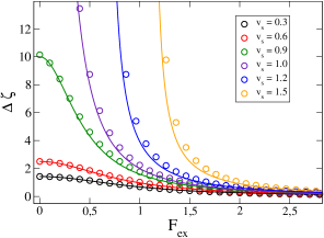
Figure 11: Friction coefficient increment from the $F_{ex}$-F1 model. The circles show the numerical values (from the direct numerical integration of eq. (164)), and the continuous lines show the analytical values (calculated from eq. (174)).

IV.7.2 $F_{ex}$-Sjögren model

For the $F_{ex}$-Sjögren model, the results of the numerical integration of eq. (164) are shown in Fig. 12 (continuous lines) as function of $F_{\rm ex}$ for different values of $\varepsilon$. We observe thinning with increasing force and see that for large forces, all the curves collapse on the same limiting curve. This limiting curve corresponds to the large $F_{ex}$ limit of the schematic model, where the $\omega$-term, which contains $F_{ex}$ dominates and the memory term can be neglected so that one obtains a $1/{F_{ex}^{2}}$ decay law for $\Delta\zeta_{s}$. This behavior also agrees with the low-density approximation in the microscopic MCT equations (see eqs. (101, 102)).

For $\varepsilon\geq 0$, the curves diverge at the critical value of force, which increases with $\varepsilon$. On the fluid side for $\varepsilon<0$, two different decay regimes can be distinguished: the strong decay from the initial (linear response) plateau for $F_{ex}<F^{c}_{ex}(\varepsilon=0)$ and the further decay for $F_{ex}>F^{c}_{ex}(\varepsilon=0)$, which approaches the $\varepsilon=0$ limiting curve with increasing force. The initial decay for $\varepsilon\rightarrow 0^{-}$ can be analyzed analytically using the $\alpha$-decay law derived in Sec. IV.6, since the time integral over the correlators is dominated by the $\alpha$-decay region for $F_{ex}<F^{c}_{ex}(\varepsilon=0)$. Relations (164), (160), (161) lead to $\Delta\zeta_{s}\approx f^{s}_{1}(F_{\rm ex})\,\int_{0}^{\infty}dt\,\tilde{\phi^{s}}\left(\frac{t}{\tau^{s}_{1}(\varepsilon,F_{\rm ex})}\right)\,\tilde{\phi}\left(\frac{t}{\tau(\varepsilon)}\right).$ From Fig. 6 (g) we see that $\phi^{s}(t)$ decays much faster than $\phi(t)$ and thus a further approximation is justified, where $\phi(t)$ is considered as constant under the integral. This gives the scaling

$$\Delta\zeta_{s}(\varepsilon,F_{\rm ex})\propto\tau(\varepsilon)\,f^{s}_{1}(F_{\rm ex})\left(\frac{f^{s}_{1}}{h_{1}}(F_{\rm ex})\right)^{1/b},$$ (178)

where the use of eq. (163) was made. The inset in Fig. 12 demonstrates the validity of the factorization of the $\varepsilon$- and the $F_{\rm ex}$-dependence in $\Delta\zeta_{s}(\varepsilon,F_{\rm ex})$: rescaling of the amplitude of the $\Delta\zeta_{s}$ vs. $F_{\rm ex}$-curves for different $\varepsilon$ leads to their coincidence. To check the $F_{\rm ex}$-scaling, we plot the function $f^{s}_{1}(F_{\rm ex})\left(\frac{f^{s}_{1}}{h_{1}}(F_{\rm ex})\right)^{1/b}$ (circles on Fig. 12; the value of the bath beta-scaling exponent $b=0.63$ was used) and observe a good agreement with the results of the direct numerical integration of eq. (164). For small $F_{\rm ex}$, the expansion $\Delta\zeta_{s}(\varepsilon,F_{\rm ex})=\Delta\zeta_{s}(\varepsilon,F_{\rm ex}=0)(1-c\,F_{\rm ex}^{2}+\mathcal{O}(F_{\rm ex}^{4}))$ is valid with $c=8.35$ (see inset in Fig. 12).

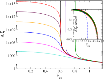
Figure 12: Main panel: friction coefficient increment from the $F_{ex}$-Sjögren model ($v_{2}=2.0$, $v_{s}=4.0$). Results from the numerical integration of eq. (164). The bold black line corresponds to $\varepsilon=0$. The values of $\varepsilon$ are $-10^{-3}$, $-10^{-4}$, $-10^{-5}$, $-10^{-6}$, $-10^{-7}$, $-10^{-8}$, 0, $10^{-4}$, $10^{-3}$ in ascending order. Inset: data for $\varepsilon=-10^{-9},\,-10^{-8},\,-10^{-7}$ (for $F_{ex}<F^{c}_{ex}$) scaled by $\tau(\varepsilon)$ to collapse onto the mastercurve eq. (178) (continuous line). The dashed line corresponds to the small $F_{\rm ex}$ expansion $\Delta\zeta_{s}(\varepsilon=-10^{-7},F_{\rm ex}=0)(1-c\,F_{\rm ex}^{2})$ (with $c=8.35$).

V Summary and Conclusions

The main objective of this work was to extend the standard mode-coupling theory for the motion of a tracer particle in a dense colloidal suspension near the glass transition to the case, where the tracer experiences an external force $F^{c}_{ex}$, which cannot be assumed to be small compared to the internal interactions of the system. This means, an attempt is made to go beyond the linear response regime. We use formally exact generalized Green-Kubo relations and follow the ideas of the integration through transients approach Fuchs and Cates (2002), recently developed for sheared systems.

The presence of the external force leads to a drastic difference compared to the linear response case: the tracer density correlator becomes complex. This is the consequence of the fact that instead of the unperturbed Smoluchowski operator $\Omega^{\dagger}_{0}$, the full operator $\Omega^{\dagger}$ containing the external force enters $\phi^{s}_{\bf q}$. $\Omega^{\dagger}$ turns out to be non-hermitian with respect to the equilibrium average, as the consequence of the fact that we consider an open system. Interestingly, in the mode-coupling theory under shear density correlators depending on advected wavevectors can be defined so as to remain real, as the affine drift motion of the particles can be taken into account rigorously. In the present case of force driven microrheology the drift motion results from the particle interactions and manifests itself in a phase factor which needs to be calculated, and which turns the correlator complex.

Despite this qualitative difference in the transient structural relaxation, in fluid states an external force gives thinning behavior of the friction coefficient akin to shear-thinning in flow. The difference to flow-driven macrorheology becomes evident in the existence of a critical force in glass states. At $F_{\rm ex}^{c}$ a continuous bifurcation transition of the long-time limit of the tracer density correlator occurs. For $F_{ex}>F^{c}_{ex}$, the long-time limit becomes zero and thus the cage surrounding the tracer breaks. The probe-particle becomes delocalized and can be pulled through the suspension.

In Sec. IV we constructed the arguably most simple schematic models by considering only two wave vectors parallel to the external force. Two different models are considered: the “$F_{ex}$-Sjögren model”, extending the Sjögren model Sjögren (1986) for the tracer coupled to a bath and the “$F_{ex}$-$F1$ model”, extending the $F1$ model of standard MCT, which was used to describe the tracer in a matrix of immobile particles (the Lorentz model). The long-time limits and the phase diagrams could be calculated analytically. The bifurcation at $F_{\rm ex}^{c}$ was shown to have codimension one.

Numerical and asymptotic solutions of the time-dependent equations of motion of the schematic models enabled predictions of the force dependence of the tracer friction increment $\Delta\zeta_{s}$. Generally, the thinning behaviour is observed similar to the shear thinning in macrorheology. For the $F_{ex}$-$F1$ model, an exact analytic expression for $\Delta\zeta_{s}$ could be derived, showing a power law divergence with the exponent $-1$ at the critical force. For the $F_{ex}$-Sjögren model, scaling laws could be given for small and large external forces.