Evidence of small-scale field aligned current sheets from the low and middle altitude cusp continuing in the ionosphere

Abstract

We investigate kilometer-scale field-aligned currents that were detected both in the magnetospheric cusp at a few Earth radii altitude and in the ionosphere by satellites that were, according to the Tsyganenko model, within a few tens of kilometers and minutes on the same magnetic field line. Also thermosphere up-welling that often accompanies the dayside field-aligned currents in the inner cusp was seen. We used Cluster and CHAMP satellites, and searched for conjunctions during the whole year of 2008, as then the Cluster spacecrafts were mostly at mid-altitudes when crossing the cusps. We focus on two case studies from this period. Evidence is presented that sheets of small scale field-aligned current continue through the low altitude cusp and ionosphere. The ionospheric current densities are not particularly strong, a few $\mu$ Am^-2 at about 340 km, and several tens of nAm^-2 at about 20000 km, implying that these currents might be relatively common events, but are hard to detect due to rareness of suitable locations of at least two satellites from different missions.

T. ZIVKOVIC, S. C. BUCHERT, H. OPGENOORTH, P. RITTER, H. LÜHR SMALL-SCALE FIELD-ALIGNED CURRENTS

T. Živković, (tatjana.zivkovic@irfu.se)

1 Introduction

The interaction between the near-Earth space and the ionosphere and upper atmosphere involves field-aligned currents (FACs) as first envisaged by [Birkeland (1913)]. The relatively large scale FAC systems of the nightside aurora have been studied and analyzed numerously, see for example, a review by [Baumjohann (1982)]. The appearance of optical aurora often suggests also the presence of small scale, less than a km wide FACs. These have indeed been found with the help of sufficiently rapidly sampling magnetometers on board of satellites in low orbits, for example, see [Lühr et al. (1994)]. The Ørstedt and CHAMP satellites, launched in 1999 and 2001, respectively, featured high-precision and fast sampling (10 and 50 Hz) fluxgate magnetometers as well as polar orbits. Perhaps a bit surprising, the most intense FACs were found with these satellites on the dayside in the cusps, reaching a few hundred $\mu$ A/m² and with scales down to a few hundred meters (Neubert and Christiansen, 2003; Watermann et al., 2003). Particularly, it was shown by Neubert and Christiansen (2003), who used Ørsted, that small-scale FACs were 1–2 order of magnitude larger than large scale region 1 and 2 currents. CHAMP is a German mission, which was flying on the altitude between 300-450 km with an inclination of $87.3^{\circ}$. Besides the Earth’s magnetic field, CHAMP, was designed to map the Earth’s gravity field and carried also an accelerometer, and was accurately tracked with GPS and satellite laser ranging. This allowed to determine accurately the satellite’s air drag. Lühr et al. (2004) showed that air drag plots from CHAMP had one dominant oscillation which was due to the air density difference on the day and night side of the Earth. Superimposed on this oscillation were relatively narrow peaks in air drag corresponding to widths of a few ten to hundred kilometers of enhanced neutral density. These thermospheric upwellings seemed to occur in the cusps and were accompanied by intense kilometer scale FACs, which were obviously causing the upwellings.

There are at least two obvious questions that deserve attention: what is the origin of the intense FACs in the cusps, and how can they cause thermospheric upwelling. In this paper mainly the first question is addressed. Watermann et al. (2008) used, in addition to magnetometer measurements of Ørsted and CHAMP, particle data from the low orbiting DMSP satellites. He showed that cusp locations as inferred from magnetosheath-like particle precipitation matched well the locations of small-scale currents, but FACs seem to be generated also in the transition zone between the low-latitude boundary layer (LLBL) and the cusp. Small scale intense FACs could also, with help of the DMSP F15 ion drift and magnetometer, be associated with very strong enhancements of the Poynting flux (Li et al., 2011). These authors proposed that magnetic reconnection in the cusp, particularly during a large $B_{Y}$ component and northward $B_{Z}$, is a cause of such small scale, but intense Poynting flux increases. Rother et al. (2007) proposed an explanation of the FACs in terms of Alfvén waves trapped in a ionospheric resonator. Then one would expect that the FACs which are observed localized in the ionosphere cannot be mapped to regions above the trapping resonator. Also, at higher altitudes, several Earth radii, localized strong FACs have been found in satellite data (Jacobsen et al., 2010). However, observations with direct evidence for ionospheric signatures of high altitude small scale FACs are rare. Here we use the Cluster spacecrafts and the CHAMP satellite to investigate whether the continuation of ionospheric small-scale current sheets can be found at much higher altitudes of a few Earth radii. The four ESA Cluster satellites were launched in 2001 with an initial perigee at 26000 km (4 RE) and apogee at 124000 km (19 RE) with orbits that relatively frequently crossed the cusps at varying altitudes. Previously, in so far only one event intense FACs were seen nearly simultaneously both in the ionosphere as well as at about 10 Earth radii distance in the outer cusp (Buchert et al., submitted, 2012). The mapping of the magnetic field using the Tsyganenko model (Tsyganenko and Stern, 1996) suggested, that the FAC seen by CHAMP might have continued all the way, and the Cluster measurements further suggested that the cause of the FAC is related to nearby ongoing magnetic reconnection. In this paper, we are particularly interested in cases where the Cluster is located at mid altitudes (a few $R_{E}$), and where chances to find FAC sheets extending over large distances from the ionosphere into near Earth space are greater than when Cluster is located in the exterior cusp.

2 Results

We have searched for conjunctions between Cluster C3 and CHAMP spacecrafts. The following criteria for a conjunction were adopted: within a time period of at most 20 minutes the difference between the geographic latitudes of the mapped Cluster footpoint and CHAMP is at most 0.5 degrees, while the difference between the geographic longitudes at most 20 degrees. Of particular interest were the conjunctions that occurred at mid altitudes, when a Cluster satellite was at about 2-3 $R_{e}$. In 2008, Cluster spacecrafts were far apart from each other and it was not possible to use results from more than one Cluster spacecraft but we have selected this year since Cluster spacecrafts crossed frequently the mid-altitude cusps.

In order to compute Cluster footprints we have used the Orbit Visualization Tool (OVT), which called the Tsyganenko 96 model (Tsyganenko and Stern, 1996) for the field line tracing. OVT is described and can be downloaded from http://ovt.irfu.se. The Cluster footprints are computed for an altitude of 120 km above the Earth, with 1 min time resolution. The CHAMP spacecraft’s circular orbit was at about 340 km altitude, and its orbital velocity was $v_{s}=7.7$ km s^-1. We have detected 11 conjunctions between Cluster C3 and CHAMP at mid altitudes in 2008, but some of these conjunctions revealed relatively weak FAC on the CHAMP satellite, probably because no intense FAC sheets were present at this time, or the CHAMP satellite orbit missed then. To investigate the interesting conjunctions further, the CHAMP fluxgate magnetometer data were used to estimate current densities. Neutral density estimates were obtained from the TU Delft thermosphere web server (http://thermosphere.tudelft.nl/acceldrag/index.php). The processing is described in Doornbos et al. (2010). Further, we use magnetic field data from the Cluster FGM instrument (Balogh et al., 2001), electric field data from the EFW instrument (Gustafsson et al., 2001), spin resolution electron spectrograms from the Plasma Electron and Current Experiment (PEACE) (Johnstone et al., 1997), as well as ion spectrograms of the precipitating particles on the Cluster CIS instrument (Rème et al., 2001). We were then left with two conjunctions for the discussion.

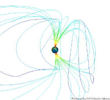
Figure 1: The 3-dimensional magnetic field according to Tsyganenko 96 during the conjunction on July 17, 2008 is plotted, the orbit of the Cluster C3 satellite is shown by a green line.

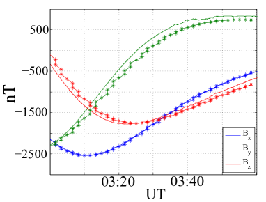
Figure 2: Magnetic field in GSE coordinates from Tsyganenko model (stars) and Cluster C3 FGM instrument.

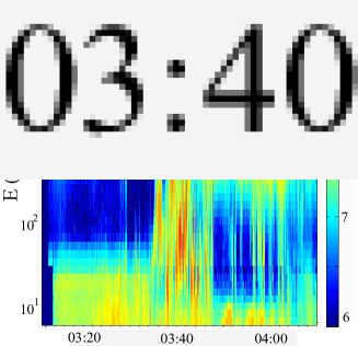
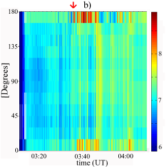
Figure 3: Electron data from the PEACE instrument in C3: a) Electron energy flux, b) Electron angular distribution (red arrow indicates current density from Figure 6.

Figure 4: Ion energy flux according to the CIS-HIA instrument.

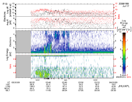
Figure 5: Ion and electron spectrograms from DMSP F13 on July 17, 2008.

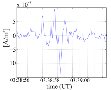
Figure 6: Current density estimates for Cluster C3.

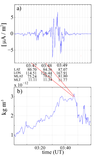
Figure 7: Estimates of a) Current density, and b) Neutral density, from the CHAMP magnetometers and accelerometers, respectively.

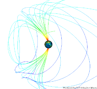
Figure 8: The 3-dimensional magnetic field according to Tsyganenko 96 during the conjunction on August 7, 2008 is plotted, the orbit of the Cluster C3 satellite is shown by a green line.

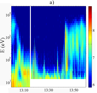
Figure 9: Electron data from the PEACE instrument in C3: a) Electron energy flux, b) Electron angular distribution (red arrow indicates current density from Figure 11).

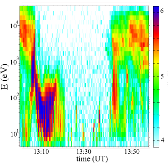
Figure 10: Ion energy flux according to the CIS-HIA instrument.

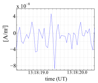
Figure 11: Current density estimates for Cluster C3.

Figure 12: Estimates of a) Current density, and b) Neutral density from the CHAMP magnetometers and accelerometers, respectively.

2.1 July 17, 2008 Cusp event

During this event the Cluster C3 spacecraft entered, according to the ion particle data (confirm Figure 4), the cusp of the Northern hemisphere at about 03:30 UT. The Tsyganenko model predicted the C3 would be on open field lines from 03:20 to 03:40 UT. Its passage is shown as a green line in Figure 1. C3 was then at an altitude of 2.8 $R_{e}$, and the mapped geographic coordinates at 03:30 UT, were 81.5 north latitude and 135.79 east longitude (MLAT: 75.24 N, MLT: 11.65). The closest other Cluster spacecraft, C1, arrived to the same area of the inner cusp 30 min earlier and, hence, could not be used for our study. At 03:47 UT, seventeen minutes after the Cluster C3 spacecraft, the CHAMP spacecraft had arrived, at 81.82 north latitude and 116.77 east longitude (MLAT: 75.24 N, MLT: 11.10). The OMNI database showed that the interplanetary magnetic field (IMF) for the period of conjunction was relatively quiet: $B_{x}$ was varying between -1 and 1 nT; $B_{y}$ was negative all the time varying between -2.2 nT and -0.3 nT, while $B_{z}$ was slightly negative, varying around $\sim-1.5$ nT. It became positive after 03:25 UT reaching maximum value of 0.7 nT. In addition, the Solar wind flow pressure was at about $\sim 1.3$ nT, and the $D_{st}\sim-13$. In order to get as precise footprints as possible, we have used the IMF, flow pressure and $D_{st}$ index starting two hours before the event, as the input parameters to the Tsyganenko model. Figure 2 shows the magnetic field at Cluster C3 and the one predicted from the Tsyganenko model at the altitude of Cluster, both in GSE coordinates. Apart from a slight disagreement in the $B_{Y}$ component, the Tsyganenko model gives good description of the magnetic field at Cluster. Figure 3a shows for the period of 03:00 to 04:10 UT the energy flux of electrons estimated from the PEACE instrument, and in Figure 3b the pitch angle distribution of the electrons is displayed. We see energies up to $1$keV with fluxes up to $10^{9}$ eV cm^-2 s^-1 sr^-1 eV^-1, which is typical for the cusp. In the period between 03:38 and 03:48 UT electrons are mostly traveling down to the ionosphere (at $180^{\circ}$), though a significant population of electrons is also traveling out of the ionosphere (at $0^{\circ}$) along the magnetic field lines. In Figure 4 ion spectrograms from Cluster C3 for the time between 03:00:00 and 04:10:00 UT are shown. High fluxes of $\sim$ keV ions are typical for the polar cusp, which gets filled by magnetosheath ions. In the same figure, a reversed ion dispersion can be seen, which is consistent with the IMF measurements. Namely, since IMF $B_{z}$ is positive, while IMF $B_{x}$ and $B_{y}$ are small, a reconnection might have occurred in the lobes, poleward of the cusp (Pitout et al., 2012). The convection of the magnetic field lines is then sunward and ion energy decreases with decreasing latitude which causes a reverse ion dispersion. This is consistent with ion velocity measurements on HIA instrument on CIS, where positive $V_{x}$ confirms that magnetic field lines convect sunward. Similar fluxes and energies of electrons and ions are measured in the same time interval on the DMSP satellite F 13, whose altitude at the time was about 850 km, and geographic coordinates were 81.2^∘ latitude and 135.1^∘ longitude. The DMSP particle spectrograms are shown in Figure 5.

From the FGM instrument on Cluster C3, we have estimated the parallel current density from 03:38:56 to 03:40:00 UT. In Figure 6, we see a positive, upward current density peak of about $90$ nAm^-2 and then negative peak of about $140$ nAm^-2. During this particular cusp crossing these current density peaks were the largest ones. The footprints for this current are 83.03^∘ north latitude and 100.43^∘ east longitude (MLAT: 76.20 N, MLT: 10.38). The signs of the current density peaks, first positive, then negative agree with the electron particle data from PEACE, see Figure 3b, where electrons first stream down to the ionosphere (an upward current) and then out of the ionosphere (a downward current). The current was estimated from the velocity of the current sheet relative to the C3 spacecraft and the magnetic field on the Cluster using Ampere’s law, $\nabla\times{\bf B}=\mu_{0}{\bf j}$ in a finite difference approximation: $\mu_{0}{\bf j}={\bf v}/(|{\bf v}|^{2}dt)\times{\bf dB}$. The FAC density is then ${\bf j}\cdot{\bf B}/|{\bf B}|$. Here ${\bf dB}$ is the difference of the magnetic field vector over the sampling interval $dt$, which is about $1/(22\mathrm{Hz})$. The velocity components of ${\bf v}$ are those measured by the ion CIS instrument. We assume that ions are moving mostly transverse to the field-line direction, and the current sheet is frozen into the plasma. Assuming that the current sheet was stationary while Cluster was passing, a current sheet width of 43 km could be estimated. The level 2 fluxgate magnetometer data from CHAMP have a time resolution of 1 s with a nominal amplitude resolution of 0.1 nT. The FAC density in the ionosphere is estimated along the satellite track from the magnetic field component perpendicular to the auroral oval, assuming stationary sheet currents (Wang et al., 2005). Positive currents flow upward. The estimated FAC density is shown in Figure 7a. Two periods of bursts of FACs can be identified: first, around 03:47:20 UT, near 81.95^∘ north latitude and 117.26^∘ east longitude (MLAT: 76.37 N, MLT: 11.17), both positive and negative currents of about 2 $\mu$Am^-2 occur. A second burst happens at 03:47:45 UT near 83.48^∘ north latitude and 122.20^∘ east longitude (MLAT: 77.78 N, MLT: 11.27). The latitude and longitude of the mapped current seen by Cluster C3 at 03:38:58 UT is close to the coordinates of CHAMP at the negative peak in this second burst. However, we believe that really the first burst at CHAMP corresponds to the current seen by Cluster C3. Firstly, the ion and electron fluxes at DMSP F13 (see Figure 5), which agree reasonably with the mapped fluxes at Cluster, are seen at a latitude close to the first current increase at CHAMP. Secondly, the small but significant difference between the Tsyganenko modeled and by Cluster measured magnetic field at 03:38 UT (see Figure 2) suggests that the footprint of Cluster is more southward than obtained from the Tsyganenko field-line tracing. Finally, we see both a positive and a negative current on Cluster and that agrees better with the positive and negative currents at CHAMP seen in first burst of FAC. Further, we can estimate how well the intensity of the current density on CHAMP corresponds to the measured current density at the Cluster C3 spacecraft. Assuming that FAC does not close between the ionosphere and Cluster altitude, and also does not connect to other transverse currents like for example polarization currents in Alfvén waves, the current density in the ionosphere $j_{i}$ should be approximately $B_{i}/B_{cl}j_{cl}$, where $B_{i}$ is the ionospheric magnetic field, $B_{cl}$ is the mean magnetic field on Cluster and $j_{cl}$ is the estimated current density at Cluster. In our case, the current density on Cluster has a positive spike of $j_{cl}\approx 9\cdot 10^{-8}$ Am^-2, which is followed by a more pronounced, negative spike of $j_{cl}\approx-1.4\cdot 10^{-7}$ Am^-2. For $B_{i}\approx 50\mu$T and a mean magnetic field on Cluster $B_{cl}$ of about 2 $\mu$T, the estimated current density in the ionosphere, should be for the positive spike $j_{i}\sim 2\cdot 10^{-6}$ Am^-2 and for the negative spike $j_{i}\sim-3.35\cdot 10^{-6}$ A/m^-2, which is slightly higher than values measured by CHAMP. If the current structure originates in the magnetosphere (for example from magnetic reconnection) then transverse diffusion of current by ion-electron collisions or wave-electron interaction would cause a widening of the structure in the ionosphere and a decrease in the current density at CHAMP. Due to the magnetic field convergence, the width of the relevant current sheet, $l$, which is 43 km at Cluster altitude, should get concentrated in the ionosphere to $l\cdot\sqrt{2\mu\mathrm{T}/50\mu\mathrm{T}}\approx$ 8.6 km. Next, we plot normalized neutral density, which is obtained from the recently calibrated accelerometer dataset from CHAMP (Doornbos et al., 2010). The density is projected to 325 km altitude as $\rho(325km)=\rho(h)\cdot\rho_{m}(325km)/\rho_{m}(h)$. Here, $\rho_{m}(h)$ is the model density according to the NRLMSISE-00 atmospheric model (Picone et al., 2002) at the satellite altitude, while $\rho$ is the measured density at the same altitude. Similar to the events reported by Lühr et al. (2004) we also see an increase of the neutral density in the time around 03:47 UT, as shown in Figure 7b.

2.2 August 7, 2008 Cusp event

During this event the Cluster C3 spacecraft, according to the ion spectrometer (compare with Figure 10), exited from the cusp of the Northern hemisphere at about 13:20 UT (and perhaps reentered later at about 13:30 UT). The Tsyganenko model predicted that C3 would be on open field lines from 12:50 to 13:25 UT. C3 was at the altitude of about 2.60 $R_{e}$. The orbit is indicated with a green line in Figure 8. Here, the CHAMP spacecraft arrived first, at 13:05 UT, within the area where according to our criteria a conjunction occurred. The geographic coordinates were latitude 79.08^∘ and longitude 302.62^∘ (MLAT: 84.57 N, MLT: 11.73). The best conjunction of Cluster 3 was at 13:18 UT, 79.16^∘ latitude and 292.44^∘ longitude (MLAT: 86.60 N, MLT: 11.08). The closest passage of any other Cluster satellite, C1, occurred 40 min earlier, and hence data from this spacecraft could not be used in our study. The IMF data from the OMNI database showed that $B_{x}\approx-2$nT, $B_{y}\approx-4$nT and $B_{z}\approx-1$nT, flow pressure $\approx$ 0.8, and $D_{st}\approx 1$. The electron spectrogram in Figure 9 a) shows energies of up to 800 eV, with fluxes of up to $10^{9}$ eV cm^-2 s^-1 sr^-1 eV^-1, which are typical values for the cusp. Figure 9 b) shows the electron distribution as a function of pitch angle. One can see that the largest population of electrons moves along magnetic field lines at around 13:15-13:20 UT, pitch angle is $180^{\circ}$, which means that electrons go down to the ionosphere. A smaller population of electrons has a pitch angle of $0^{\circ}$. From the ion spectrogram in Figure 10, we see the ion dispersion characteristic for the southward IMF, where less energetic ions stream along more poleward magnetic field lines when the reconnection occurs at the dayside magnetopause. Further, we estimate the parallel current density at C3 the same way as for the first event (see Figure 11). The strongest current density increase occurs at around 13:18:19 UT, and that is also the strongest current density increase in the period that Cluster C3 stayed in the cusp. A burst of a few $\mu$Am^-2 strong currents started at CHAMP (see Figure 12 a) with the most intense current around 13:04:00 UT, at about 75.22^∘ north latitude and 298.89^∘ east longitude (MLAT: 81.93, MLT: 10.39). In this event, the magnetic field of the Tsyganenko model and the one measured by Cluster C3 deviate considerably, particularly in the $B_{Y}$ and $B_{Z}$ components (not shown here). There is no obvious explanation why the Tsyganenko model is relatively unrealistic in this case, as the event under study occurred under very quiet geomagnetic and solar wind conditions. Nevertheless, moderately strong FACs are seen on both Cluster and CHAMP within about 14 minutes in areas that are within some uncertainty conjugate to each other. For the ionospheric magnetic field of $B_{i}\sim 50\mu$T, an average magnetic field on Cluster of $B_{cl}\sim 2.1\mu$T and the positive current density estimated for Cluster of $j_{cl}\sim 4.5\cdot 10^{-8}$ Am^-2, the ionospheric current density should be $j_{i}\sim 1.13\cdot 10^{-6}$ A/m^-2. The negative current density estimated on Cluster is $j_{cl}\sim-8\cdot 10^{-8}$ Am^-2, which gives the ionospheric current density of $j_{i}\sim-2\cdot 10^{-6}$, which agrees well with the positive and negative current measured at CHAMP at 13:04:00 UT. The width of current sheet at Cluster is estimated to be about $6.5$ km. Then a sheet width of only about $1.3$ km is expected in the ionosphere at CHAMP altitude which is below the resolution of the available magnetic data. Nevertheless, the neutral density (normalized to 325 km) increases also here when CHAMP crossed the region where thin current sheet in the ionosphere was located, i.e. at around 13:05 UT. This is shown in Figure 12b). Note that here the peak in density should be related to the FAC burst, but one cannot expect a 1-1 correspondence because of a field-line inclination and a motion of FAC during upwelling time.

3 Discussion and Conclusion

We have shown two cases of small-scale field-aligned currents which stretch from the magnetosphere through the ionosphere inside the polar cusp. These current sheets are identified in the magnetosphere with the Cluster C3 spacecraft, and in the ionosphere with the CHAMP spacecraft. These currents seem quite ”geo-effective”, since they heat the ionosphere and upper atmosphere and cause upwelling of the thermosphere. It has been pointed out already by Lühr et al. (2004), that the density enhancements accompanied by small-scale field-aligned currents occur quite independently of magnetic activity. Also these events occured under only moderate or quiet geomagnetic and solar wind conditions. A similar study has been carried by Buchert et al., submitted (2012), where the “same” current sheet was suggested to be seen both by Cluster and CHAMP spacecraft. However, in that study, Cluster spacecrafts were in the exterior cusp and the distance between them and CHAMP were about 60000km, while the distance between Cluster and CHAMP in our case study is less than 20000km. Buchert et al., submitted (2012) also observed that ions flow up from the ionosphere to the magnetosphere, apparently as a consequence of field-aligned electron current which was coming from the magnetosphere. For both case studies in this paper, we have checked densities and directions of oxygen ions measured from the CODIF CIS instrument on Cluster, because these ions are usually coming from the ionosphere. No oxygen ions in periods of the formation of electron current sheets could be detected. Most of the ions detected on the CIS instrument were due to hydrogen which was originally coming from the magnetosphere. So at least in these two cases no ionospheric outflow was detected. Without additional acceleration the ionospheric upflow would ballistically return to the ionosphere (Ogawa et al., 2009), or it would take the ions of the order of hours to reach an altitude of roughly 20000 km. Therefore we think that the failure to detect oxygen outflow here is explained by the absence of energization of ions in the topside ionosphere. This could be related to the low magnetic activity conditions in these events. In addition, we have noticed that in one event the Tsyganenko model field agreed well with the observed one, while in the other there was a relatively large discrepancy between model and observation in spite of low activity and low Cluster altitude.